Math, Statistics, and Data › Linear Algebra I: Vectors and Matrices › Day 99
Day 99: Vectors: Direction, Magnitude, and Meaning
After this lesson you will be able to look at a row of numbers describing one thing — a colour, a house, a customer, a document — and recognise it as a vector you have been using for ninety-eight days without the name; hold both pictures of it at once, as a list you type and as an arrow with a direction and a length, and say exactly which of the two survives the jump to three hundred dimensions and which does not; add, subtract and scale vectors both geometrically and componentwise, and explain the parallelogram; derive the magnitude from Pythagoras rather than accepting it as a formula, and compute it by hand for vectors whose answer is a whole number; normalise a vector and state precisely what that changes and what it preserves; compute the L1 norm alongside the L2 and produce a case where the two rank the same pair of candidates in opposite orders; compute the distance between two vectors as the magnitude of their difference and see why there was never a separate formula; implement add, subtract, scale, dot, both norms, distance, normalise and nearest-neighbour search in pure Python, then prove operation by operation that NumPy agrees with your loops on the same inputs; write every float assertion with a stated tolerance and demonstrate on your own machine why double-equals would have failed; and then take six short articles, turn them into vectors by counting, compute every pairwise distance and say — precisely, numerically, and with the working shown — which one is most like which.
Hands-on lab for this lesson
Lab files on GitHub: https://github.com/ai-roadmap-365/ai-roadmap-365.github.io/tree/main/labs/sections/math-statistics-and-data/day-099-vectors-direction-magnitude-and-meaning
- Get the hands-on files. Clone the labs repository once (you can reuse this clone for every lesson). This works on macOS, Linux, and Windows (PowerShell or WSL):
git clone https://github.com/ai-roadmap-365/ai-roadmap-365.github.io.git cd ai-roadmap-365.github.io - Open this lesson's lab. Move into the directory for this specific day. Every lab lives at the same predictable path — section / subsection / week / day:
cd labs/sections/math-statistics-and-data/day-099-vectors-direction-magnitude-and-meaning - Read the lab guide. Open `README.md` in that directory. It lists the exact commands, what each does, the expected output, and how to check your work — read it before running anything.
- Run it and check your work. Follow the README's "How to run" section: run the example first to see the finished result, then complete the numbered exercises in `starter/`, then run the tests. The tests pass (exit 0) only when your work is correct.
bash tests/run_tests.sh # or the test command named in the lab README
You can also open the lab as a local page (works offline, shows the file tree and expected output).
Learning objectives
By the end of this lesson you will be able to:
- Recognise a vector in data you already have: a row of numbers describing one thing, where position carries meaning and the order can never change
- Hold the two pictures of a vector at once — an ordered list and an arrow with direction and magnitude — and name what each one is good for
- State exactly which intuitions survive the jump from 2D and 3D to hundreds of dimensions, and which are lost along with the drawing
- Add and subtract vectors componentwise and geometrically, and explain the parallelogram picture and why the order of addition does not matter
- Multiply a vector by a scalar, and say what a positive, a negative and a zero scalar each do to direction and to magnitude
- Derive the L2 norm from Pythagoras rather than asserting it, and compute magnitudes by hand for vectors whose answer is a whole number
- Normalise a vector, explain why normalising is so common in practice, and produce a case where it changes which item wins a search
- Compute the L1 norm alongside the L2, and construct a concrete case where the two norms rank the same two candidates in opposite orders
- Compute the distance between two vectors as the norm of their difference, and explain why there is no separate distance formula to learn
- Compute a dot product, state that it returns a single number, and use a dot product of zero to identify perpendicular vectors
- Describe the zero vector and the standard basis, and explain what it means that a coordinate list is already a combination of basis vectors
- Implement every operation in pure Python from first principles, then prove agreement with NumPy operation by operation to a stated tolerance
- Assert every floating-point comparison with math.isclose or numpy.allclose and a tolerance you state, having demonstrated on your own machine why double-equals fails
- Turn six short documents into vectors by counting features, compute every pairwise distance, and name each one nearest neighbour with the arithmetic shown
- Compare pure Python lists, NumPy arrays, PyTorch tensors, JAX arrays and pandas Series for this work, and explain why NumPy is the shape the others imitate
Prerequisites
- Day 43 to 46 — Python functions, lists, comprehensions, and floating-point arithmetic; Day 46 in particular, because today is where "never compare floats with double-equals" stops being advice and becomes a failing test
- Day 51 — modules and imports, which is how the lab example scripts find the implementation you write
- Day 63 — pytest, and what a parametrised test does
- Day 83 — virtual environments and pinned requirements, which is how the lab installs its two dependencies
- School arithmetic: squares, square roots, and the fact that a right triangle with sides 3 and 4 has a hypotenuse of 5. Nothing beyond that is assumed, and nothing beyond that is needed
Why this matters
Open a spreadsheet you already have. Pick any row.
Ashfield,3,4A place, and two numbers: three kilometres east of the depot, four kilometres north. That row is a vector. You have not learned anything new, you have not converted anything, and nothing needs installing. The row was already a vector on the day somebody typed it.
Here is another one:
#1D4ED8 -> (29, 78, 216)That is the blue used in this course’s diagrams, as three numbers: red 29, green 78, blue 216. A colour is a vector. You have been writing vectors since Day 1.
And here is a third:
roast-chicken,9,0,1,0Four numbers counting how many times a short article mentions cooking, running, money and weather. Also a vector, and this is the one that matters, because when a language model turns a sentence into a list of 384 numbers, it is producing exactly this object. Bigger, and with columns nobody chose by hand — but the same object, with the same operations available.
Ninety-eight days of this course have been about instructing a computer. This day is where you start describing the world to one. Everything in the second half of this course — embeddings, semantic search, similarity, gradients, weights, attention — is built on the idea that a thing can be a list of numbers and that two things being alike means their lists being close.
That word “close” is the whole day. It sounds soft. It is not. By the end of this page you will be able to take six articles, turn them into vectors by counting, and say — with the squares, the sum and the square root written out — that roast-chicken and slow-cooker-stew are 1.4142 apart while roast-chicken and household-budget are 11.3137 apart. Not “more similar”. 1.4142 against 11.3137.
Let me be blunt about the fear, because a lot of readers arrive at this section of the course expecting to be found out.
You do not need any mathematics beyond school arithmetic to do today’s work. You need squares, you need square roots, and you need to be willing to write out four lines of addition. Every single worked example on this page is computed in full, and every number in it comes out whole or is shown to four decimal places from a real run. Nothing is asserted and left hanging. If a formula appears, it appears after the arithmetic that produced it, never before.
What the day costs if you skip it is specific, and it lands later:
- You will not be able to debug a search that returns the wrong thing. When a retrieval system ranks an article about marathons above your recipe, the cause is almost never the model. It is that raw counts made a short query look near the shortest document rather than the most similar one. You will meet exactly that failure in this lab, with numbers.
- You will write a test that fails on correct code. Normalising a vector gives a magnitude of 1 — except that on the machine this lesson was written on, three of seven test vectors came out at
0.9999999999999999. A test written with==fails, and you will spend an afternoon looking for a bug that is not there. - You will not be able to say what your own results mean. “Nearest” is undefined until you name a norm. This page contains two candidates where one norm says A is nearer and the other says B is nearer, both correct. A result that does not name its norm is a result you cannot defend.
The good news is the shape of the day. You will implement all of it — addition, subtraction, scaling, dot product, both norms, distance, normalisation, nearest-neighbour search — in about forty lines of plain Python with no libraries at all. Then you will run the same operations through NumPy on the same inputs and prove they agree. The order is deliberate. A reader who has written the loop knows what the library is doing before being asked to trust it, and that is the difference between using NumPy and being at its mercy.
The idea in plain language
A vector is an ordered list of numbers where position means something.
That is the whole definition. Read it twice, because most of the difficulty people have with this subject comes from expecting it to be harder.
- Ordered — the list has a first, a second, a third.
(3, 4)and(4, 3)are different vectors describing different places. - List of numbers — no text, no gaps, just numbers.
- Position means something — slot 1 is always east, slot 2 is always north. Swap two columns of your dataset and every row now means something else.
There is a second picture of the same object, and this is where the subject gets its reputation. A vector is also an arrow: something with a direction and a length. Three east and four north is a walk, and a walk has a direction (roughly north-east) and a distance (five kilometres as the crow flies).
Both pictures are correct and they are the same object. The point of today is holding them together.
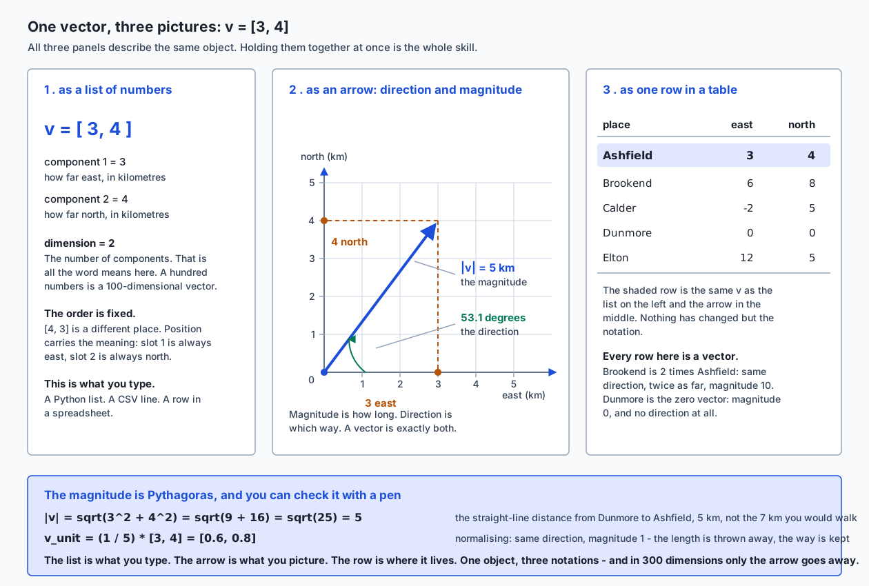
Look at the three panels of that diagram and notice that nothing changes between them but the notation:
| Picture | What it is good for | Where it fails |
|---|---|---|
The list (3, 4) | Typing, storing, computing. It is what a CSV row, a Python list and a database record already are | It gives no feel for what the numbers mean together |
| The arrow | Intuition. Direction, length, “these two point the same way” — all obvious at a glance | It only exists in two or three dimensions. In 384 dimensions there is nothing to draw |
| The row in a table | Seeing that a dataset is a collection of vectors, one per thing | It hides the geometry: rows look like records, not like points in a space |
The last row of that table is the one people miss. A spreadsheet with 500 rows and 12 numeric columns is not “data that could be turned into vectors”. It is 500 points in a 12-dimensional space, right now, and asking which two customers are most alike is asking which two of those points are closest — a question with an arithmetic answer.
Here is the claim the rest of the day cashes out:
An embedding is a vector, and “similar things are near each other” is a statement about distance that you will be able to compute by hand before you finish this page.
Not a metaphor. A distance, in the ordinary sense: subtract, square, add, take the square root.
Historical background
Vectors are younger than you would expect, and the reason is instructive: for two thousand years mathematics had the geometry without the notation.
Euclid’s Elements, written in Alexandria around 300 BC, contains in Book I, Proposition 47 the result the whole of today rests on — that in a right-angled triangle the square on the hypotenuse equals the sum of the squares on the other two sides. Every magnitude you compute today is that proposition, applied one dimension at a time. What Euclid did not have was a way to write “the thing that goes three east and four north” as an object you could add to another object.
That notation arrived in the 1840s, and it arrived twice.
William Rowan Hamilton, in Dublin, was trying to extend complex numbers to three dimensions and failing for years. On 16 October 1843, walking along the Royal Canal to a meeting of the Royal Irish Academy, he saw that it worked in four dimensions rather than three, and carved the defining relation of the quaternions into the stone of Broom Bridge. Quaternions have four parts, and Hamilton called the three-part directional piece the vector part — from the Latin vehere, to carry — and the single-number piece the scalar part. Both words are his, and both survive today with meanings slightly narrower than he intended.
Independently and almost simultaneously, Hermann Grassmann, a schoolteacher in Stettin, published Die lineale Ausdehnungslehre in 1844. Grassmann’s work was more general and more modern than Hamilton’s — it is closer to what a linear algebra course teaches now — and it was almost entirely ignored for decades, partly because it was written in a philosophical style that even sympathetic mathematicians found impenetrable.
The vector notation you actually use was assembled in the 1880s by Josiah Willard Gibbs at Yale and Oliver Heaviside in England, working separately and both motivated by the same practical problem: quaternions were clumsy for physics, and electromagnetism needed something cleaner. They stripped the quaternion down, kept the three-component directional object, and defined the dot product and the cross product as separate operations rather than as parts of one quaternion multiplication. Gibbs printed his lecture notes privately for his students; Heaviside published his in the electrical engineering literature. The resulting notation won a bad-tempered argument with the quaternion school in the 1890s and became the standard.
Giuseppe Peano gave the modern axiomatic definition of a vector space in 1888, in Calcolo geometrico, which is what makes it legitimate to say that a list of 384 numbers is a vector even though it is not an arrow in any space you can see.
The idea of measuring distance by adding absolute differences rather than by Pythagoras — what this page calls the L1 norm — is associated with Hermann Minkowski, who studied families of distance functions of this kind around the turn of the twentieth century. The nickname “taxicab” or “Manhattan” distance came much later and from the obvious picture: on a street grid you cannot go through the buildings.
The computational history is much shorter. Jim Hugunin wrote Numeric in 1995 while a graduate student, giving Python its first array object. A decade of divergence followed, with a competing package called Numarray, and Travis Oliphant unified the two into NumPy, released as version 1.0 in 2006. Almost everything numerical in Python since then either is NumPy or imitates its interface deliberately — which is why the last section of this lesson can describe PyTorch, JAX and pandas mostly by saying what they changed about it.
One thing worth noticing in all of that: the arithmetic came first, the geometry was known for millennia, and the notation — the ability to write one letter for a whole list and manipulate it — is the recent invention. That is a fair description of what you are learning today. You already knew how to add two numbers. What you are gaining is the ability to stop writing the loop.
What it is — and what it is not
Let me clear away the misconceptions individually, because each one blocks something later.
| Misconception | What is actually true |
|---|---|
| ”A vector is an arrow, so it needs 2 or 3 dimensions” | An arrow is one picture of a vector, available in 2D and 3D only. The definition — an ordered list of numbers — has no such limit. A 384-component embedding is as much a vector as (3, 4) is |
| ”A vector has to start at the origin” | It does not. In the flow diagram below, the arrow from (2, 2) to (5, 6) is a perfectly good vector — it is (3, 4), the same vector as the one from the origin to (3, 4). A vector is a displacement, not a location. Two arrows are the same vector when they have the same direction and length, wherever they are drawn |
| ”A vector and a point are different things” | They are different interpretations of the same list. (3, 4) as a point is a place; as a vector it is the journey from the origin to that place. Code does not distinguish them, and you should not lose sleep over it — but the difference is why subtracting two points gives a vector while adding two points is a slightly odd thing to do |
| ”Dimension is a physical thing” | Dimension is a count. It means “how many numbers are in this list”. A vector of a hundred sales figures is 100-dimensional, and there is nothing spatial about it |
| ”Magnitude can be negative” | Never. It is a square root of a sum of squares, so it is zero or positive. A negative component is fine; a negative magnitude is a bug |
| ”Normalising cleans up the data” | Normalising does exactly one thing: sets the magnitude to 1 while keeping the direction. It is not scaling to a 0-1 range, it is not standardising, it is not removing outliers. Those are different operations with different names |
| ”The zero vector points somewhere by default” | It has magnitude 0 and no direction at all. Attempting to normalise it is a genuine error, and a function that returns a list of nan instead of saying so has made your bug invisible |
| ”Vectors need a library” | You will implement every operation on this page in plain Python in about forty lines. NumPy is for speed and convenience, not capability |
And two things a vector genuinely is not:
It is not a matrix. A matrix is a rectangle of numbers; a vector is a single list. A table of many vectors stacked up is a matrix, which is Day 100’s subject, and the relationship between the two is the reason these days are adjacent.
It is not automatically meaningful. A vector is a list of numbers, and whether the distance between two of them means anything depends entirely on whether the columns were chosen sensibly and measured in comparable units. If component 1 is a price in pounds and component 2 is an age in years, the distance between two rows is a number with no interpretation whatsoever — it is adding squared pounds to squared years. This is the single most common way to produce a confidently wrong result with vectors, and no amount of correct arithmetic will save you from it.
Why it was created and what problems it solves
Gibbs and Heaviside were not doing housekeeping. They wanted to solve a problem that arises the moment you have several quantities that belong together.
Consider what you have to write without vector notation. A force in three dimensions is three numbers. Adding two forces means writing three separate equations. Adding twenty forces means sixty equations, and the fact that they are all the same equation is invisible on the page. Now imagine an embedding with 384 components and you can see why the notation is not cosmetic: it lets you write one line where you would otherwise write hundreds, and it makes the sameness of those lines explicit.
The problems vectors solve, concretely:
1. Grouping things that belong together. A colour is not three unrelated numbers, it is one colour. A position is not two unrelated numbers. The moment you name the group, you can pass it around, store it, compare it and operate on it as a unit — and your code stops carrying x, y and z as three parameters that can get out of step.
2. Making “how different are these two things” computable. This is the big one for this course. Two rows of numbers, one subtraction and one square root, and you have a number. Not a judgement — a number that ranks, sorts, thresholds and gets asserted in a test.
3. Making the same code work in any number of dimensions. Look at what is absent from every formula on this page: the dimension. The magnitude is “square every component, add, take the root” — however many components there are. That is why the pure-Python functions you write today will work unchanged on a 384-component embedding.
4. Separating “which way” from “how far”. A vector carries both, and normalisation is the operation that keeps one and discards the other. This matters more in practice than it sounds. A long document has bigger word counts than a short one on the same topic. Length is an artefact; direction carries the topic. Normalising deletes the artefact.
5. Turning meaning into geometry. This is the modern reason and it is why this day sits where it does in the course. If you can arrange things so that similar items get nearby vectors, then searching by meaning becomes searching by distance — and searching by distance is something a computer is very good at.
How it works
Here is the machinery, in order, with every number computed.
Throughout, I will use the map: a depot at the origin, and places reached by walking east and north. v = (3, 4) means three kilometres east, four north.
Adding two vectors
Add matching components:
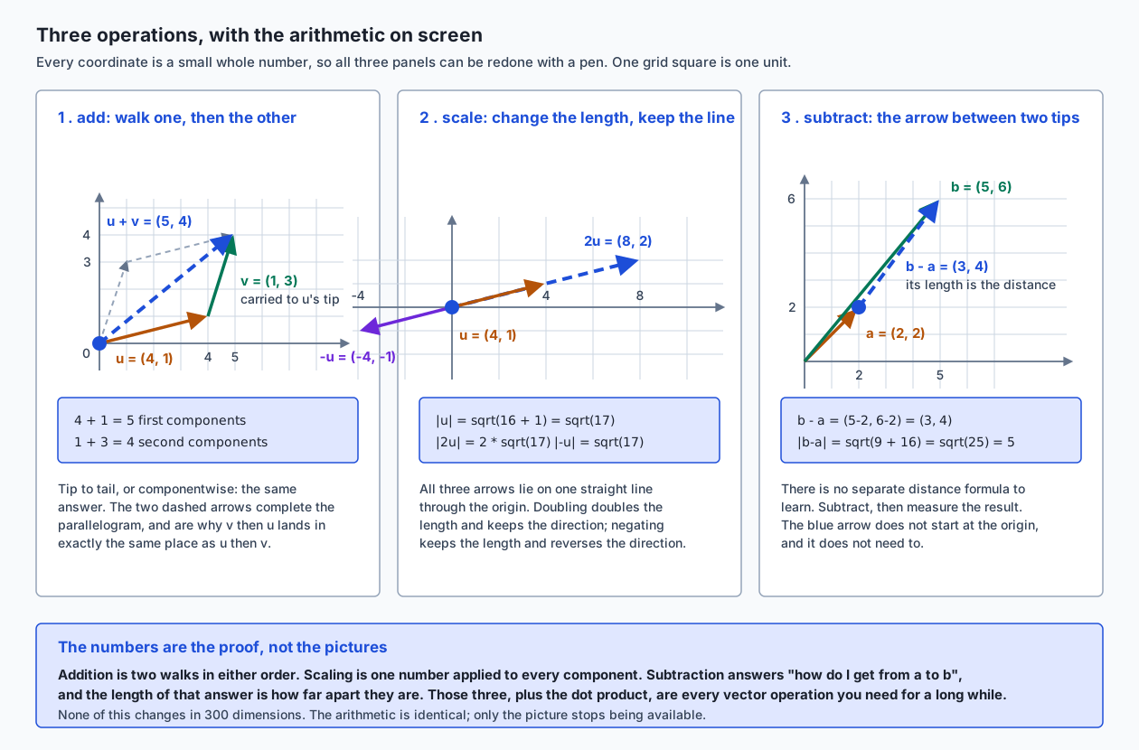
u = (4, 1)
v = (1, 3)

u + v = (4 + 1, 1 + 3) = (5, 4)
Geometrically: walk u, then from wherever you land walk v. Draw v starting at the tip of u — “tip to tail” — and the arrow from the start of u to the tip of v is the sum.
Now do it the other way round: walk v first, then u. You get (1 + 4, 3 + 1) = (5, 4). The same place. Draw both routes and they form a parallelogram: two sides are copies of u, two are copies of v, and the sum is the diagonal. That is the parallelogram picture, and it is a picture of a fact you can also see in the arithmetic — 4 + 1 and 1 + 4 are the same number, so addition of vectors is commutative because addition of numbers is.
Subtracting two vectors
Subtract matching components:
b = (5, 6)
a = (2, 2)

b - a = (5 - 2, 6 - 2) = (3, 4)
Geometrically, and this is the sentence to memorise: b - a is the arrow that starts at the tip of a and ends at the tip of b. It answers “how do I get from a to b”. Notice it does not start at the origin. It does not need to.
Hold on to that, because in three paragraphs it becomes the definition of distance.
Multiplying by a scalar
Multiply every component by the same number:
u   = (4, 1)
2u  = (8, 2)
-u  = (-4, -1)
0u  = (0, 0)
What changes and what does not:
Scalar k | Direction | Magnitude |
|---|---|---|
k > 1 | unchanged | multiplied by k — longer |
0 < k < 1 | unchanged | multiplied by k — shorter |
k = 0 | destroyed — the result is the zero vector | 0 |
k < 0 | reversed | multiplied by ` |
All the scaled copies lie on one straight line through the origin. That is worth pausing on: scaling never leaves the line, which is why “the direction of v” is a property shared by every positive multiple of v, and why normalising can pick one canonical representative of that whole family.
The zero vector
(0, 0), or (0, 0, 0), or 384 zeros. Its properties:
- Adding it changes nothing:
v + 0 = v. It is the additive identity. - You get it by scaling anything by 0, or by subtracting a vector from itself.
- Its magnitude is 0.
- It has no direction at all — not “direction zero”, not “pointing along the first axis”, none. And therefore it cannot be normalised, because normalising means dividing by the magnitude and the magnitude is zero.
That last point is a real bug source. In this lab, normalise([0, 0, 0]) raises a ValueError with a message saying so. NumPy, given the same division, returns array([nan, nan, nan]) with a runtime warning — and nan is not equal to anything, including itself, so it silently poisons every comparison downstream. Both behaviours are defensible; what is not defensible is not knowing which one your code does.
Magnitude, derived rather than asserted
Now the important one, and I am going to derive it rather than write it down.
You have walked 3 km east and 4 km north. How far are you from the depot in a straight line?
Draw it. The eastward leg and the northward leg meet at a right angle — east and north are perpendicular, that is what they mean — so you have a right-angled triangle whose two short sides are 3 and 4, and whose hypotenuse is the straight-line distance you want. Euclid, Book I, Proposition 47:
hypotenuse^2 = 3^2 + 4^2
             = 9 + 16
             = 25

hypotenuse   = sqrt(25)
             = 5
Five kilometres. And notice you would walk seven — three plus four — because you cannot go through the fields. Remember that gap; it comes back as the L1 norm.
Now three dimensions. Add “and then 12 km up”, giving (3, 4, 12). Apply Pythagoras twice: the first two legs give a horizontal distance of 5, and that 5 is perpendicular to the vertical 12, so:
|v|^2 = 5^2 + 12^2 = 25 + 144 = 169
|v|   = 13
But look what that is in terms of the original numbers:
|v|^2 = (3^2 + 4^2) + 12^2 = 9 + 16 + 144 = 169The same answer. Adding a dimension just adds another squared component to the sum. There is nothing special about three, and the argument repeats for four, for five, for 384. So:
The magnitude of a vector is the square root of the sum of the squares of its components.
This is called the L2 norm, and when anyone says “the norm” or “the length” or “the magnitude” without qualification, this is what they mean. Written |v|.
Four you can check with a pen right now:
| Vector | Squares | Sum | Magnitude |
|---|---|---|---|
(3, 4) | 9, 16 | 25 | 5 |
(6, 8) | 36, 64 | 100 | 10 |
(2, 3, 6) | 4, 9, 36 | 49 | 7 |
(1, 2, 2) | 1, 4, 4 | 9 | 3 |
(3, 4, 12) | 9, 16, 144 | 169 | 13 |
(7, 1, 5, 3, 9, 2) | 49, 1, 25, 9, 81, 4 | 169 | 13 |
That last row is six-dimensional and you just computed its magnitude with a pen. You cannot draw it. It did not matter.
Two consequences fall straight out:
- Signs vanish.
(-3, -4)has magnitude 5, the same as(3, 4), because squaring removes the sign. A magnitude tells you how far, never which way. - Magnitude is never negative. It is a square root of a sum of squares.
Distance: there is no second formula
Here is the moment that makes most of linear algebra stop looking like a list of things to memorise.
You know how to subtract two vectors: b - a is the arrow from a to b. You know how to measure the length of a vector. So:
The distance between
aandbis the magnitude ofb - a.
Subtract, then measure. That is all.
a = (2, 2)
b = (5, 6)

b - a       = (3, 4)
|b - a|     = sqrt(3^2 + 4^2) = sqrt(9 + 16) = sqrt(25) = 5
The distance is 5. If you have ever seen the “distance formula” written out as a square root of a sum of squared differences and found it arbitrary, this is where it comes from — it is not a separate rule, it is the norm applied to a difference.
Three properties, all checkable and all asserted in the lab’s test suite:
- Symmetric.
distance(a, b) = distance(b, a), becausea - bisb - areversed and reversing does not change length. - Zero only for identical points.
distance(a, a) = |0| = 0. - The triangle inequality.
distance(a, c) <= distance(a, b) + distance(b, c). Going via a third point is never a short cut. This is one of the conditions a function has to satisfy before anyone is allowed to call it a distance.
The L1 norm, and where it disagrees
Go back to the walk. Straight-line distance from the depot to (3, 4) is 5 km. But you walked 3 + 4 = 7 km, because the streets run east-west and north-south and you cannot cut the corner.
That 7 is the L1 norm: add up the absolute values of the components. No squaring, no square root.
L1 of (3, 4)     = |3| + |4|         = 7
L2 of (3, 4)     = sqrt(9 + 16)      = 5

L1 of (1, 2, 2)  = 1 + 2 + 2         = 5
L2 of (1, 2, 2)  = sqrt(1 + 4 + 4)   = 3
Both answer “how big is this vector”. Both are correct. They are different questions.
The difference is not decorative, and here is the case that proves it. A query sits at the origin. Two candidates:
spike  = (4, 0, 0)     one large component
spread = (2, 2, 2)     three small ones
Compute both norms for both:
spike   L1 = 4 + 0 + 0 = 4
        L2 = sqrt(16 + 0 + 0) = sqrt(16) = 4

spread  L1 = 2 + 2 + 2 = 6
        L2 = sqrt(4 + 4 + 4) = sqrt(12) = 3.4641...
Under L2, spread is nearer (3.4641 < 4). Under L1, spike is nearer (4 < 6). The two norms rank the same pair in opposite orders.
Squaring is what does it. In L2 a single component of 4 contributes 16 to the sum, while three components of 2 contribute only 4 each. So L2 punishes one large deviation far more than it punishes the same total spread thinly, whereas L1 counts every unit at face value and does not care how it is distributed.
| L2 (Euclidean) | L1 (taxicab, Manhattan) | |
|---|---|---|
| Formula | sqrt(sum of squares) | sum of absolute values |
| Everyday picture | as the crow flies | walking a street grid |
| Effect of one big component | punished heavily (squared) | counted at face value |
| Effect of many small components | forgiven (small squares) | counted in full |
| Relation | never larger than L1 | never smaller than L2 |
| Typical use | the default for distance and similarity | chosen when one large deviation should not dominate |
| Smoothness | smooth everywhere, easy to differentiate | has a corner at zero in each component |
Use L2 unless you have a reason. But state which one you used, because as you have just seen, a ranking can flip.
Unit vectors and normalisation
A unit vector has magnitude 1. It carries direction and nothing else.
To get one, scale by one over the magnitude:
v      = (3, 4)
|v|    = 5
v_unit = (1/5) * (3, 4) = (0.6, 0.8)

check: sqrt(0.6^2 + 0.8^2) = sqrt(0.36 + 0.64) = sqrt(1.0) = 1
Because the scalar 1/5 is positive, the direction is untouched. Only the length changed, from 5 to 1. This is worth saying precisely because it is a favourite exam question and a genuine source of confusion: normalising changes magnitude and preserves direction. Scaling the unit vector back up by 5 returns (3.0, 4.0), which is the check that direction really did survive.
Why is normalising so common in practice? Because length is very often an artefact and direction is the signal.
Take the lab’s catalogue. roast-chicken has feature counts (9, 0, 1, 0). Now imagine the same article written at three times the length — the same topic, the same balance, more words:
short = (9, 0, 1, 0)      magnitude 9.0554
long  = (27, 0, 3, 0)     magnitude 27.1662

raw distance between them        = 18.1108
distance after normalising both  = 0.0000
On raw counts, those two articles are eighteen units apart, which would be a serious claim about their content. They are about the identical thing. The long one is the short one scaled by 3, so after normalising they are literally the same vector and the distance is exactly 0. Length was the entire disagreement.
The dot product
Multiply matching components, add the results, return one number:
u = (1, 2, 3)
v = (4, 5, 6)

u . v = 1*4 + 2*5 + 3*6 = 4 + 10 + 18 = 32
Two lists go in; one number comes out. That collapse is why the dot product is everywhere — a weighted sum, a projection, and a similarity score are all this operation under different names, and it is the single most common thing a machine learning model does, several billion times per query.
Two facts to carry forward:
- A dot product of zero means the two vectors are perpendicular.
(1, 0) . (0, 1) = 0.(3, 4) . (-4, 3) = -12 + 12 = 0. - The dot of a vector with itself is its magnitude squared.
(3, 4) . (3, 4) = 9 + 16 = 25 = 5^2. Which is another way of saying the L2 norm issqrt(v . v).
Basis vectors, and what a coordinate actually is
One last idea, and it explains why any of this notation means anything.
In two dimensions, define:
e1 = (1, 0)     one step east, nothing north
e2 = (0, 1)     nothing east, one step north
Then:
3 * e1 + 4 * e2 = (3, 0) + (0, 4) = (3, 4) = vSo writing v = (3, 4) was already shorthand for “three of the first basis vector plus four of the second”. A coordinate list is a set of instructions relative to a chosen set of reference directions. That set is called a basis, and e1, e2 is the standard basis.
Why this matters, in one sentence: the numbers depend on the basis, the vector does not. Choose different reference directions — measure along the road and across it rather than east and north — and the same physical journey gets a different pair of numbers. Nothing about the journey changed. This is the seed of the idea that a matrix is a change of point of view, which is where the next few days go.
The honest jump to high dimensions
Everything above was demonstrated in two and three dimensions because those can be drawn. Embeddings have hundreds. What comes with you?
| Idea | Survives to 384 dimensions? |
|---|---|
| The definition: an ordered list of numbers | Yes. Unchanged |
| Addition, subtraction, scaling, componentwise | Yes. Unchanged |
| Magnitude = root of sum of squares | Yes. The formula never mentioned the dimension |
| Distance = magnitude of the difference | Yes. Unchanged |
| Dot product, and dot of zero meaning perpendicular | Yes. Unchanged |
| The triangle inequality | Yes. Still holds |
| Normalising to magnitude 1 | Yes. Unchanged |
| The picture — arrows, angles seen by eye | No. There is nothing to draw |
| ”Perpendicular” as something you can visualise | No, though the arithmetic still works. Vectors in high dimensions are overwhelmingly likely to be close to perpendicular, which is not what 2D intuition expects |
| ”Most points are close to at least a few others” | No. High-dimensional space is far emptier than intuition suggests, and distances between random points bunch together |
The last two rows are the honest caveats and they have a collective name in the literature: the curse of dimensionality. Today’s arithmetic is exact and unaffected. What is affected is how much a nearest-neighbour result means when everything is roughly the same distance from everything else — which is a real problem in retrieval systems and one of several reasons embeddings are trained rather than hand-counted.
For now, take the good news: every formula on this page is dimension-free, and you verified all of them with a pen.
An everyday analogy
The analogy has been running underneath the whole lesson, so let me make it explicit and then push it until it breaks, because an analogy you have not broken is an analogy you do not understand.
A vector is a journey.
- The list
(3, 4)is the instruction: go three east, four north. - The direction is which way you end up facing relative to where you started.
- The magnitude is how far you are from where you started, as the crow flies. Five kilometres.
- Adding two journeys is doing one and then the other. The order does not matter, which is why the parallelogram closes.
- Subtracting answers “how do I get from where you are to where I am”.
- Scaling by 2 is the same journey, twice as far. Scaling by −1 is walking back.
- The zero vector is not going anywhere. You end where you started, and there is no meaningful answer to “which way did you face” — which is exactly why it cannot be normalised.
- Normalising is answering “which way is Ashfield from here?” with a compass bearing instead of a distance. You have deliberately thrown away how far.
- The L1 norm is how far you actually walk on a street grid — seven kilometres. The L2 norm is how far the crow flies — five. Both are real answers to “how far”, and which one you want depends on whether you have wings.
- The distance between two places is the length of the journey between them, which is why you subtract first.
Where the analogy breaks, and it is worth knowing:
Journeys are three-dimensional at most; vectors are not. There is no walk corresponding to a 384-component embedding, and no bearing you could point at. When you get to embeddings, keep the arithmetic and drop the walking.
Journeys happen in a space that exists independently; embeddings do not. East and north are real directions in a real world that would be there without you. The 384 components of an embedding are whatever a training process produced, they have no individual meaning, and the space has no privileged directions. The consequence: “nearby” in embedding space means “the model placed these near each other”, not “these are objectively similar”. That distinction matters enormously when a search result is wrong, because the answer is not out there to be found — it was manufactured.
Kilometres are all the same unit; your columns may not be. If component 1 is a price and component 2 is an age, then sqrt(price^2 + age^2) is adding squared pounds to squared years and the result means nothing at all. The map analogy quietly assumes every component is measured the same way, and real datasets very often are not. The fix — rescaling columns to comparable ranges — is a whole subject of its own, and the thing to carry today is the awareness that the assumption is there.
Examples in practice
Time to build the thing the day promised. Six short articles, turned into vectors by counting, and a program that says which is most like which.
The catalogue
Four features, counted by hand: how many times each article mentions cooking, running, money and weather.
| article | cooking | running | money | weather | magnitude |
|---|---|---|---|---|---|
roast-chicken | 9 | 0 | 1 | 0 | 9.0554 |
slow-cooker-stew | 8 | 0 | 2 | 0 | 8.2462 |
marathon-plan | 0 | 9 | 1 | 2 | 9.2736 |
race-day-nutrition | 4 | 6 | 3 | 0 | 7.8102 |
household-budget | 1 | 0 | 9 | 0 | 9.0554 |
storm-bulletin | 0 | 1 | 0 | 9 | 9.0554 |
That is a hand-made embedding. Real ones are produced by a trained model and have hundreds of components whose meanings nobody assigned. Everything else — one row of numbers per item, nearness measured with a norm — is the same.
Two distances, worked out in full
roast-chicken against slow-cooker-stew:
(9, 0, 1, 0) - (8, 0, 2, 0) = (1, 0, -1, 0)

squares:  1 + 0 + 1 + 0 = 2
sqrt(2) = 1.4142
roast-chicken against household-budget:
(9, 0, 1, 0) - (1, 0, 9, 0) = (8, 0, -8, 0)

squares:  64 + 0 + 64 + 0 = 128
sqrt(128) = 11.3137
1.4142 against 11.3137. That is what “these two are similar and those two are not” means, numerically, and you can redo both on paper.
One more, and this one comes out exactly whole:
household-budget vs race-day-nutrition
(1, 0, 9, 0) - (4, 6, 3, 0) = (-3, -6, 6, 0)

squares:  9 + 36 + 36 + 0 = 81
sqrt(81) = 9
The full distance matrix
Captured from a real run of examples/embeddings.py in the lab:
                      roast-chi  slow-cook  marathon-  race-day-  household  storm-bul
roast-chicken            0.0000     1.4142    12.8841     8.0623    11.3137    12.8062
slow-cooker-stew         1.4142     0.0000    12.2474     7.2801     9.8995    12.2474
marathon-plan           12.8841    12.2474     0.0000     5.7446    12.2474    10.6771
race-day-nutrition       8.0623     7.2801     5.7446     0.0000     9.0000    11.4455
household-budget        11.3137     9.8995    12.2474     9.0000     0.0000    12.8062
storm-bulletin          12.8062    12.2474    10.6771    11.4455    12.8062     0.0000
The diagonal is zero — every article is zero distance from itself — and the matrix is symmetric about it, because distance is symmetric. Both of those are checks, not decorations: if either failed you would have a bug.
Nearest neighbours
  roast-chicken        -> slow-cooker-stew     at 1.4142
  slow-cooker-stew     -> roast-chicken        at 1.4142
  marathon-plan        -> race-day-nutrition   at 5.7446
  race-day-nutrition   -> marathon-plan        at 5.7446
  household-budget     -> race-day-nutrition   at 9.0000
  storm-bulletin       -> marathon-plan        at 10.6771
Read those and check them against your own judgement. The two cooking articles pair up, tightly. The two running-adjacent articles pair up. And then the interesting ones: household-budget’s nearest neighbour is race-day-nutrition at 9.0000, and storm-bulletin’s is marathon-plan at 10.6771 — both large distances, and both essentially saying “nothing here is much like me”. The number carries that information. A ranking without the number would not.
Where raw counts go wrong, and normalising fixes it
Now the failure worth seeing. A one-line note: “roast it”. Its vector is (1, 0, 0, 0) — one mention of cooking, nothing else.
Which article should it match? Obviously roast-chicken, the article most purely about cooking. Here is what actually happens, from the real run:
  article                 raw distance   normalised distance
  ----------------------------------------------------------
  roast-chicken                 8.0623                0.1106
  slow-cooker-stew              7.2801                0.2444
  marathon-plan                 9.3274                1.4142
  race-day-nutrition            7.3485                0.9878
  household-budget              9.0000                1.3338
  storm-bulletin                9.1104                1.4142

  nearest on raw counts : slow-cooker-stew at 7.2801
  nearest normalised    : roast-chicken at 0.1106
  raw rank of roast-chicken        : 3
  normalised rank of roast-chicken : 1
On raw counts, roast-chicken comes third — behind slow-cooker-stew and behind race-day-nutrition, which is mostly about running. That is a wrong answer produced by entirely correct arithmetic.
The cause: the query vector is short, so it sits near the origin, and raw distance measured from near the origin is dominated by how long each article is rather than by what it is about. Length is competing with topic, and length is winning. Normalising puts every vector on the unit sphere, deletes length from the comparison, and leaves only direction. Normalised, roast-chicken wins at 0.1106 and race-day-nutrition falls to 0.9878.
Two details in that table reward a second look. marathon-plan and storm-bulletin both come out at exactly 1.4142 — the square root of 2 — from the cooking query. That is not a coincidence: both mention cooking zero times, so their unit vectors have a dot product of exactly 0 with the query’s unit vector, which is to say they are perpendicular to it. Perpendicular unit vectors are always sqrt(2) apart. The dot product and the distance are telling you the same thing in two languages.
The from-scratch implementation
Here is the whole of it, in plain Python, no imports beyond math. This is examples/vectors.py from the lab, condensed:
import math

def check_same_dimension(u, v):
    if len(u) != len(v):
        raise ValueError(f"dimension mismatch: {len(u)} and {len(v)}")

def add(u, v):
    check_same_dimension(u, v)
    return [a + b for a, b in zip(u, v)]

def subtract(u, v):
    check_same_dimension(u, v)
    return [a - b for a, b in zip(u, v)]

def scale(k, v):
    return [k * a for a in v]

def dot(u, v):
    check_same_dimension(u, v)
    total = 0.0
    for a, b in zip(u, v):
        total += a * b
    return total

def l2_norm(v):
    return math.sqrt(sum(a * a for a in v))

def l1_norm(v):
    return sum(abs(a) for a in v)

def distance(u, v):
    return l2_norm(subtract(u, v))

def normalise(v):
    length = l2_norm(v)
    if length == 0.0:
        raise ValueError("cannot normalise the zero vector: it has no direction")
    return scale(1.0 / length, v)
That is the entire subject of this lesson, executable. Notice three deliberate choices:
The dimension guard is separate and called explicitly. Adding a 2-vector to a 3-vector is not a slightly wrong answer, it is a meaningless question, and zip would silently truncate to the shorter one and return something plausible. Silence is the failure mode to avoid.
distance is one line built from two others. It is not a formula, it is a composition, and writing it that way makes the fact unforgettable.
normalise raises on the zero vector. It could have returned nans. It does not, because a loud error at the point of the problem is worth ten hours of debugging later.
And then NumPy — which does the same thing
Now the same operations through the library, on the same inputs, from a real run of examples/agreement.py (numpy 2.5.2):
operation             pure Python                       NumPy                             agree
-----------------------------------------------------------------------------------------------
add(u, v)             [4.0, 2.0, 17.0]                  [4.0, 2.0, 17.0]                  True
subtract(u, v)        [2.0, 6.0, 7.0]                   [2.0, 6.0, 7.0]                   True
scale(k, u)           [7.5, 10.0, 30.0]                 [7.5, 10.0, 30.0]                 True
negate(u)             [-3.0, -4.0, -12.0]               [-3.0, -4.0, -12.0]               True
zero(3)               [0.0, 0.0, 0.0]                   [0.0, 0.0, 0.0]                   True
normalise(u)          [0.230769, 0.307692, 0.923077]    [0.230769, 0.307692, 0.923077]    True
dot(u, v)             55.0                              55.0                              True
l2_norm(u)            13.0                              13.0                              True
l1_norm(u)            19                                19.0                              True
distance(u, v)        9.433981132056603                 9.433981132056603                 True
l1_distance(u, v)     15                                15.0                              True

every operation agrees: True
u = (3, 4, 12), v = (1, -2, 5), k = 2.5. Every comparison used numpy.allclose(rtol=1e-9, atol=1e-12) or math.isclose with the same tolerance — never ==, for reasons two sections down.
In NumPy the same eleven operations are written like this:
import numpy as np

u = np.array([3, 4, 12])
v = np.array([1, -2, 5])

u + v                            # add
u - v                            # subtract
2.5 * u                          # scale
np.dot(u, v)                     # dot product
np.linalg.norm(u)                # L2 norm
np.linalg.norm(u, ord=1)         # L1 norm
np.linalg.norm(u - v)            # distance
u / np.linalg.norm(u)            # normalise
That is the payoff for having written the loops. np.linalg.norm(u) is not magic; it is math.sqrt(sum(a * a for a in v)) with a faster inner loop.
And NumPy adds two things the loops do not, both captured from the same run:
1. A whole table of vectors is one object, and one call measures every row:
     matrix shape        = (3, 4)
     norms of all rows   = [9.0554 8.2462 9.2736]
     the same, by loop   = [9.0554, 8.2462, 9.2736]
     agree               = True

2. Every distance from one query to every row, in one expression:
     query               = [1, 0, 0, 0]
     distances (NumPy)   = [8.0623 7.2801 9.3274]
     distances (loop)    = [8.0623, 7.2801, 9.3274]
     agree               = True
The second is the one that matters. stacked - query subtracted a four-component vector from every row of a 3-by-4 table without a loop. That is broadcasting, and it is why a similarity search over a million embeddings is a few lines rather than a nested loop.
The floating-point trap, demonstrated
Normalise a vector and its magnitude is 1. Write the test:
assert l2_norm(normalise(v)) == 1.0Here is what happened when that was actually checked on seven vectors, from the real run of examples/normalise.py:
vector                    |v|                   |v_hat| (exact repr)      == 1.0   isclose
------------------------------------------------------------------------------------------
[3, 4]                    5.0                   1.0                       True     True
[1, 2, 2]                 3.0                   1.0                       True     True
[1, 1]                    1.4142135623730951    0.9999999999999999        False    True
[1, 1, 1]                 1.7320508075688772    1.0                       True     True
[0.1, 0.2, 0.3]           0.37416573867739417   0.9999999999999999        False    True
[2, 3, 6]                 7.0                   0.9999999999999999        False    True
[7, 1, 5, 3, 9, 2]        13.0                  1.0                       True     True

exactly 1.0 : 4 of 7
isclose 1.0 : 7 of 7
Four passed == 1.0. Three failed. The maths is correct in every single row — every one of them is 1.0 to within rel_tol=1e-9. Only the equality test disagrees.
Look at (2, 3, 6), which is the sharpest case in the table. Its magnitude is exactly 7.0 — a whole number, exactly representable in binary — and dividing by it still does not give back exactly 1.0 when you square and add the results.
Day 46 explained why: a float is a binary approximation, and a chain of divisions and multiplications can land one unit in the last place away from the exact answer. Today is where it bites, and the lesson is not “floats are broken”. It is:
Every floating-point comparison needs a stated tolerance, and a test written with
==will fail on correct code.
Use math.isclose(value, 1.0, rel_tol=1e-9, abs_tol=1e-12) or numpy.allclose(a, b, rtol=1e-9, atol=1e-12). Both parts matter: rel_tol scales with the size of the numbers, and abs_tol is what saves you near zero where a relative tolerance is meaningless. State them out loud rather than leaning on a library default — NumPy’s default rtol is 1e-05, which is far looser than most people assume when they call allclose and move on.
The lab’s test suite contains a test whose only job is to prove this on the machine it runs on. It asserts that all seven are 1.0 to tolerance, and that at least one of them is not exactly 1.0. If that second assertion ever stops holding somewhere, the harness fails loudly rather than letting the lesson quietly tell a lie.
Implications: security, privacy, performance, scalability, and cost
Performance. The pure-Python functions above are correct and slow. Every operation walks a Python list one element at a time, with the interpreter’s overhead on each step. NumPy stores the numbers in one contiguous block of memory in a fixed type and runs the loop in compiled code, often using the processor’s vector instructions to handle several components per cycle. The gap is large — commonly one to two orders of magnitude, and larger for big arrays — but it depends heavily on array size, dtype and hardware, so the lab’s extension exercise asks you to measure the ratio on your machine rather than quote a number you read. What is not in doubt is the shape: correctness comes from the loop you wrote, speed comes from the library.
Scalability. Comparing a query against a million embeddings of 384 components each is 384 million multiply-adds per query, which is fast in compiled code but not free, and it grows linearly with the collection. This is why vector databases exist and why approximate nearest-neighbour indexes exist: they trade a small chance of missing the true nearest item for a search that does not touch every row. That trade-off is a later subject. What today gives you is the ability to say precisely what such an index is approximating.
Memory and cost. A 384-component embedding stored as 32-bit floats is 1,536 bytes. A million of them is about 1.5 GB before any index. That is a real infrastructure number and it comes straight out of dimension times bytes per number. Halving the precision to 16-bit floats halves it and costs some accuracy; the fact that this is even a decision is worth knowing before somebody presents it to you as a foregone conclusion.
Privacy — the important one. It is very tempting to assume that turning a document into 384 floating-point numbers has destroyed the original. It has not. Research on embedding inversion has repeatedly recovered substantial portions of source text from its embedding. Treat an embedding of personal data as personal data: same access controls, same retention policy, same deletion obligations. “It is only numbers” is not an argument, and a deletion request that removes a document but leaves its vector in an index has not been honoured.
Security. Three consequences follow from what you learned today:
- A vector store is a database. Who can read it, who can write to it, is it encrypted at rest, what happens on a deletion request — all the usual questions apply, and none of them get easier because the contents look like noise.
- Nearest-neighbour rankings leak. If a search returns the closest documents to a query and some of those documents are ones the user is not allowed to see, then the ranking itself is a disclosure: you learn that something exists and roughly what it resembles without ever being shown it. Access control belongs in the retrieval step, not in the rendering step.
- A similarity threshold compared with
==is a decision an attacker can nudge. “Is this similarity above 0.95?” is a gate, and a gate whose comparison is unstable at the last bit is a gate with a wobble in it. The float discipline you learned today is a correctness practice in a lab and a security practice in production.
Cost of getting the modelling wrong. Nothing in the arithmetic will stop you computing sqrt(price^2 + age^2). It will return a number. That number is meaningless, and no amount of correct code will tell you so. Whether the components of your vector are comparable is a judgement you have to make, and it is the most expensive mistake available in this area precisely because it produces confident, plausible, wrong answers.
Alternatives: free, open source, and commercial
For the work on this page, here is the landscape. I ran the first two. I did not run the last three, and no output from them is reproduced anywhere in this lesson or lab — they are described from their published documentation, and the lab’s test harness confirms they are not installed so that this statement cannot quietly rot.
| Option | Licence and cost | Choose it when | Do not choose it when |
|---|---|---|---|
| Pure Python lists | Free, standard library | Learning; small data; when the dependency is not worth it; when you want to be certain what the code does | Any array of real size — it is one to two orders of magnitude slower and you will feel it |
| NumPy 2.5.2 | Free, BSD-3-Clause. No paid edition exists | Essentially always, for numerical work on one machine. It is the default and the thing everything else imitates | You need automatic differentiation, or GPU execution, or data larger than memory |
| PyTorch | Free, BSD-style. Paid only in the sense that the cloud GPUs you run it on cost money | You need gradients or a GPU. Tensors behave like NumPy arrays deliberately | Plain numerical work with no learning involved — it is a large dependency for np.linalg.norm |
| JAX | Free, Apache-2.0. Same cloud-cost caveat | You want NumPy semantics plus composable transformations — automatic differentiation, just-in-time compilation, vectorised mapping | You need in-place mutation or a small footprint; its arrays are immutable by design |
| pandas | Free, BSD-3-Clause | Your vectors are rows of a labelled table and you care about the labels, the joins and the missing-value handling | You are doing pure vector arithmetic — it adds an index and an axis-alignment layer you did not ask for |
Ran here, with output reproduced:
Pure Python lists. Every operation on this page, forty lines, math.sqrt the only import. Concrete example: l2_norm([3, 4, 12]) returns 13.0. Free, no install, and it is what the lab asks you to write.
NumPy 2.5.2. Installed in the lab’s pinned environment and run for every agreement check above. Concrete example, from the real run:
>>> import numpy as np
>>> np.linalg.norm([3, 4, 12])
13.0
and the broadcast form that makes it worth having:
>>> matrix = np.array([[9, 0, 1, 0], [8, 0, 2, 0], [0, 9, 1, 2]])
>>> np.linalg.norm(matrix - np.array([1, 0, 0, 0]), axis=1).round(4)
array([8.0623, 7.2801, 9.3274])
Described from documentation only, nothing run:
PyTorch tensors. The documented interface is deliberately NumPy-shaped: a tensor is created with torch.tensor([3.0, 4.0, 12.0]), added with +, scaled with *, and measured with torch.linalg.norm, with torch.dot for the dot product. Two documented differences carry the whole reason it exists. A tensor can live on a GPU (.to("cuda")), and a tensor created with requires_grad=True records the operations performed on it so that gradients can be computed backwards through them. When you meet gradient descent later in this course, that second feature is the one doing the work. Free and open source; the cost is the hardware you run it on.
JAX arrays. The documented interface is closer still — jax.numpy is written to mirror the NumPy API, so jnp.linalg.norm(x) is spelled the way you would expect. The documented differences are that arrays are immutable, so an in-place update is written as a functional x.at[i].set(value) returning a new array, and that the library’s value is in transformations you wrap around your function: grad for derivatives, jit for compilation, vmap for automatic vectorisation. Free and open source.
pandas Series. A Series is a one-dimensional labelled array. Per its documentation, arithmetic between two Series aligns on the index rather than on position — which is a genuinely different model from everything else here, and the source of most surprises for people arriving from NumPy. It is the right tool when your vector is a named row of a table with a schema, and the wrong tool when you want raw positional arithmetic. Free and open source.
Why NumPy is the one everything else imitates. Two reasons, and neither is inertia.
First, it got the core abstraction right and early: a fixed-type, contiguous, N-dimensional array with a shape, plus broadcasting rules that make an operation between different-shaped arrays mean something predictable. That combination is what lets matrix - query do the obviously-intended thing, and every library since has adopted it rather than invented a rival.
Second, and more importantly, the interface became a lingua franca. Because SciPy, scikit-learn, pandas, Matplotlib and the rest all speak arrays, a new library that speaks a different dialect has to justify itself against an enormous existing ecosystem. PyTorch and JAX did not copy NumPy’s spelling out of politeness; they copied it because doing otherwise would have cost their users everything they already knew. When a library says “NumPy-compatible API”, it is making a promise about the size of the thing you do not have to relearn.
Comparison with related concepts
| Concept | What it is | How it relates to a vector |
|---|---|---|
| Scalar | A single number | Multiplying a vector by one scales it. The word exists to distinguish “the plain number” from “the list” in an expression |
| Point | A location | The same list, differently interpreted. A point is where you are; a vector is a displacement. Subtracting two points gives a vector — this is why b - a is the arrow from a to b |
| Matrix | A rectangle of numbers | A stack of vectors, and also a transformation that turns vectors into other vectors. Day 100 |
| Array (programming) | A container of same-typed values | The implementation. A NumPy 1-D array is a vector as far as today is concerned; the word is about storage, not meaning |
| List (Python) | An ordered, mutable container of anything | A list of numbers works as a vector and is what the lab uses. It can also hold strings, so “list” is broader and less specific than “vector” |
| Tuple / record / row | A fixed group of fields | A row of a table with all-numeric fields is a vector. If any field is text, it is not — until somebody encodes the text as numbers, which is what embedding is |
| Embedding | A learned vector representing an item | A vector, produced by a model rather than by hand, arranged so that similar items are near each other. Today’s arithmetic is exactly what “near” means |
| L2 norm | Root of sum of squares | The magnitude. The default meaning of length, size and distance |
| L1 norm | Sum of absolute values | An alternative magnitude. Can rank two candidates in the opposite order to L2, as shown above |
| Cosine similarity | The dot product of two unit vectors | Distance after normalising, in different clothes: for unit vectors, squared distance equals 2 - 2 * cosine. It is what people reach for when direction matters and length does not, which is most of the time in text retrieval |
| Dot product | Sum of componentwise products | Returns a scalar, not a vector. Zero means perpendicular. Underneath cosine similarity, projections, and most of what a model computes |
| Basis | Reference directions the coordinates are measured against | Every coordinate list is already a combination of basis vectors. Change the basis, the numbers change, the vector does not |
The comparison worth dwelling on is L2 distance against cosine similarity, because in text retrieval you will see both and people rarely explain the relationship. If both vectors are normalised to magnitude 1, they are two views of one thing: cosine similarity 1 corresponds to distance 0, cosine 0 to distance sqrt(2), cosine −1 to distance 2. That is exactly the sqrt(2) you saw earlier between the cooking query and the two articles that mention cooking zero times — perpendicular, cosine 0, distance sqrt(2). If the vectors are not normalised, the two measures can genuinely disagree, and the whole of the raw-versus-normalised table above is that disagreement made visible.
When to use it — and when not to
Reach for vector thinking when:
- You have several numbers that describe one thing and belong together — a colour, a location, a set of measurements, a row of counts.
- You want to ask “how similar are these two things?” and get a number rather than an opinion.
- You need to rank a collection against a query.
- You are working with anything a model produced as a list of numbers: an embedding, a set of weights, a gradient.
- The same computation has to work in 2 dimensions today and 384 tomorrow.
Be careful when:
- The components are in different units.
sqrt(pounds^2 + years^2)is not a quantity. Either rescale the columns to comparable ranges first, or accept that the distance means nothing. This is the failure that produces confident nonsense. - The components are not really numbers. A category encoded as 1, 2, 3 is not a number: it silently claims that category 3 is three times category 1 and twice as far from category 1 as category 2 is. Distances over such a column are meaningless.
- Length is an artefact of your process rather than a property of the thing. Longer documents have bigger counts. Normalise, or explain why you did not.
- The dimension is very high and the collection is small. In high dimensions everything is roughly equidistant from everything else, so “nearest” may be true but uninformative. Look at the actual distances, not just the ranking —
storm-bulletin’s nearest neighbour at 10.6771 is telling you something quite different fromroast-chicken’s at 1.4142.
Do not reach for it when:
- The data is genuinely relational. “Which members borrowed a book by an author who also wrote X” is a join, not a distance. Days 85 to 91 covered the right tool, and turning that question into a vector problem makes it worse.
- You need an exact match. Nearest-neighbour search returns the closest, which is not the same as the correct. If you are looking up an order by its reference number, use an index.
- You need to explain the answer to a regulator. “These two vectors are 0.31 apart” is not a reason a decision can be justified with. That is not an argument against using vectors, it is an argument for knowing what you can and cannot claim from one.
- A simple rule already works. If a
WHEREclause answers the question, a distance calculation is not an improvement.
Knowledge check
Eight questions accompany this lesson in quiz.yml. Two of them are the ones that separate a reader who has understood the day from one who has read it: the question about what normalising changes and what it preserves, and the question about why assert l2_norm(normalise(v)) == 1.0 is wrong. If either of those is not immediately obvious, reread the normalisation section and then run examples/normalise.py in the lab and look at the seven rows it prints.
Before you take it, try answering these from memory:
- What are the two pictures of a vector, and which one stops working in 384 dimensions?
- Why is the magnitude of
(3, 4)equal to 5, and where does that argument come from? - Why is there no separate distance formula?
- What does a positive scalar do to direction? A negative one?
- Give a pair of vectors where L1 and L2 disagree about which is nearer to the origin.
- What is the dot product of
(3, 4)and(-4, 3), and what does the answer tell you? - Why can the zero vector not be normalised?
- What is wrong with
assert norm == 1.0, and what should it say instead?
Hands-on exercise
Build the vector library yourself, then prove it agrees with NumPy.
The lab is at labs/sections/math-statistics-and-data/day-099-vectors-direction-magnitude-and-meaning/. Read starter/00_brief.md first — it has the table of six articles, four answers to check yourself against on paper, and the floating-point trap stated in advance so it is a lesson rather than an ambush.
Install and start:
cd labs/sections/math-statistics-and-data/day-099-vectors-direction-magnitude-and-meaning
python3 -m venv .venv
.venv/bin/pip install -r requirements/requirements.txt
.venv/bin/python3 starter/vectors.py
Then implement the nine numbered exercises in starter/vectors.py, in order — add, subtract, scale, dot, l2_norm, l1_norm, distance, normalise, nearest. Each is a few lines. After each one, delete the @pytest.mark.skip line above its test in starter/test_starter.py and run:
.venv/bin/pytest starter -qDo not import NumPy in starter/vectors.py. The whole point is that you write the loop first; the test harness checks that you did.
Expected output
Before you write anything:
Day 099 starter — Vectors You Can Hold

  1. add          not started
  2. subtract     not started
  3. scale        not started
  4. dot          not started
  5. l2_norm      not started
  6. l1_norm      not started
  7. distance     not started
  8. normalise    not started
  9. nearest      not started

0 of 9 exercises return something.
1 passed, 11 skippedWhen you have finished all nine and removed all eleven skip markers:
12 passedAnd the full harness, from the lab directory:
87 checks, 0 failure(s).Validate your work
.venv/bin/python3 starter/vectors.pyreports9 of 9 exercises return something..venv/bin/pytest starter -qreports12 passed..venv/bin/pytest tests -qreports79 passed— the reference suite, which your implementation is not required to satisfy but which you should read.cd examples && ../.venv/bin/python3 byhand.pyends withall exact cases agree: True.cd examples && ../.venv/bin/python3 agreement.pyprintsevery operation agrees: True.cd examples && ../.venv/bin/python3 normalise.pyprintsisclose 1.0 : 7 of 7and anexactly 1.0count lower than 7. If yours reads7 of 7, the trap did not reproduce on your machine — record that, because it is a real finding about your platform rather than a failure.bash tests/run_tests.sh; echo $?ends with87 checks, 0 failure(s).and prints0. Check the exit status directly rather than through a pipe, because a pipeline reports the last command’s status and not the harness’s.
Troubleshooting
ModuleNotFoundError: No module named 'numpy' — you are running a Python without the lab’s dependencies. Create the .venv above and run everything through .venv/bin/python3.
TypeError: object of type 'NoneType' has no len() — an earlier exercise still returns None and a later one is calling it. distance needs subtract and l2_norm; nearest needs distance. Work in order, and run python3 starter/vectors.py to see which are unfinished.
A test fails with a bare assert False — that is close(...) returning False. Print the value: if l2_norm([3, 4]) gives 25.0 you forgot the square root; if it gives a list you returned the squares instead of their sum.
ValueError: dimension mismatch: 2 and 3 — working as intended. You combined a 2-vector with a 3-vector, which is a meaningless question rather than a slightly wrong answer.
ValueError: cannot normalise the zero vector — also working as intended.
Your normalisation assertion fails but the maths looks right — you almost certainly wrote == 1.0. Run examples/normalise.py and look at the three rows that come out at 0.9999999999999999.
The lab’s troubleshooting.md has the full list, with every error message quoted from a run that actually produced it.
Common mistakes
- Forgetting the square root in
l2_norm. The most common error in the exercise, and it passes a surprising number of casual eyeball checks because the ranking of distances is unchanged — only the values are wrong. The harness catches it by asserting the exact magnitudes. - Returning a list from
dot. The dot product sums the componentwise products. If you return the products, you have written a different (also useful) operation. - Writing a separate distance formula. If
distancedoes not callsubtractandl2_norm, you have missed the day’s central point even if the answer is right. - Comparing floats with
==. Covered at length. It will pass for(3, 4)and fail for(1, 1). - Letting
ziphide a dimension mismatch. Without the guard,add([1, 2], [1, 2, 3])returns[2, 4]— a plausible, silent, wrong answer. - Normalising the zero vector without noticing. Either raise, or return
nans knowingly. Do not find out by accident three functions downstream. - Assuming raw counts are comparable. The one-line query that ranks
roast-chickenthird exists in the lab precisely so you meet this before it costs you something.
Practice assignment
Extend the catalogue and defend a design decision with numbers.
-
Add a seventh article. Invent it, count its four features by hand, and add it to
CATALOGUEin your own copy. Before running anything, write down which existing article you predict will be its nearest neighbour, and why. Then run it. If you were wrong, work out which component drove the answer — being wrong here is more instructive than being right. -
Implement cosine similarity. Add
cosine_similarity(u, v)asdot(normalise(u), normalise(v)). Compute it for all fifteen pairs of the original six articles. Then prove the relationship stated in this lesson: for unit vectors,distance^2 = 2 - 2 * cosine_similarity. Assert it withmath.iscloseand a stated tolerance, for every pair. -
Write the norm decision down. Compute every pairwise distance under L1 as well as L2. Find a pair of articles that the two norms rank differently relative to some third article — or, if there is no such pair in this catalogue, say so and show the working that establishes it. Then write two sentences recommending one norm for this task and stating what you gave up.
-
Break your own tolerance. Set
REL_TOLto1e-18instarter/test_starter.pyand run the suite. Which tests fail? Are those failures about your code or about floating point? Now set it to1e-1and ask which real bugs would slip through. Write down, in one sentence, what a tolerance is actually trading off.
Deliverable: your modified starter/vectors.py, a short findings.md with your prediction and what actually happened, the cosine table, and the two-sentence norm recommendation. Every number quoted must come from a run you performed.
Extension challenge
Build a working semantic search over real text — with no model.
Take twenty short text files of your own: notes, articles, anything. Then:
-
Build the vocabulary. Split each file into lowercase words, drop the fifty most common words across the whole collection (they carry almost no signal), and keep the next 200 as your feature columns. That gives every document a 200-dimensional vector of counts.
-
Vectorise and normalise. Turn each document into its 200 counts, then normalise. Report the magnitude of each document before normalising, and note the range — that spread is exactly the document-length artefact this lesson warned about.
-
Search. Take a query string, turn it into a vector with the same vocabulary, normalise it, and return the five nearest documents by L2 distance. Print the distances, not just the ranking.
-
Measure the failure honestly. Find a query where the result is wrong — you will not have to look hard, because word counting has no idea that “run” and “running” are related, or that “bank” means two things. Write down what a trained embedding would have to know in order to get that query right. This is the clearest possible statement of what an embedding model buys you, and you will have earned it by watching counting fail.
-
Compare implementations. Do step 3 twice: once with your pure-Python loop over all twenty documents, once with a single broadcast NumPy expression. Assert that the two agree to a stated tolerance, then time both with
time.perf_counterand report the ratio you measured on your machine. Then scale up: generate 10,000 random 200-dimensional vectors and time it again. Report both ratios and note whether they are the same.
Two rules. Every number in your write-up must come from a run you performed, and every float comparison must state its tolerance.
The AI thread
This is the day the second half of this course becomes possible, and it is worth saying plainly rather than gesturing at.
An embedding is a vector. When a model turns a sentence into 384 or 1,536 numbers, it is producing the object you spent today measuring. Nothing about the arithmetic changes — the magnitude is still the square root of the sum of the squares, the distance is still the norm of the difference, and you can still compute both with the functions you wrote this morning. What the model provides is not new mathematics, it is better columns: instead of four features somebody counted by hand, hundreds of features learned from text, arranged so that nearness corresponds to meaning rather than to shared vocabulary.
Semantic search is nearest-neighbour search by distance. Embed the documents, embed the query the same way, return the items whose vectors are closest. That is the whole idea, and you implemented it today over six articles. Everything harder about it in production is one of two things: getting better vectors, or avoiding the need to measure every single row.
A model’s weights are vectors. The parameters of a neural network are numbers arranged in vectors and matrices, and training consists of changing them a little at a time.
A gradient is a vector. When you meet gradient descent, the gradient will be a vector pointing in the direction in which the error increases fastest — and “direction”, “magnitude” and “scale by a small number then subtract” will all mean exactly what they meant today. The learning rate is a scalar. The update step is a subtraction. You have already met every operation involved.
And one thing that is not a technical point but is the reason this section of the course exists. A great deal of published work in this area presents distances and similarity scores as though they were measurements of the world. They are not. They are consequences of a chosen representation, a chosen norm, and a chosen preprocessing pipeline — three decisions, each of which you made explicitly today and each of which changes the answer. You saw a query where raw counts ranked the right article third and normalising put it first. You saw two candidates where L1 and L2 disagreed about which was nearer.
Knowing that those are decisions, rather than facts, is most of what separates someone who can use these systems from someone who can only believe them.
Quiz
Q1. A colleague says "we cannot use vectors here, our data is just a spreadsheet of customers with twelve numeric columns each". What is the most accurate reply?
- They are right — vectors are arrows in 2D or 3D, and twelve columns cannot be drawn, so the word does not apply
- Each row already is a 12-dimensional vector; the word adds a set of operations, not a new kind of data
- The spreadsheet would first have to be normalised before any row could be called a vector
- Only the numeric columns count, so it depends on whether any of the twelve are text
Show answer
Answer: B. Each row already is a 12-dimensional vector; the word adds a set of operations, not a new kind of data
A vector is an ordered list of numbers where position carries meaning, and a spreadsheet row with twelve numeric columns is exactly that. Nothing needs converting; the only thing that changes is that a family of operations — add, subtract, scale, measure, compare — becomes available, and questions like "which two customers are most alike?" become arithmetic rather than opinion. Option 0 is the most common and most damaging misconception: the arrow picture is a picture, useful up to three dimensions and gone after that, but the definition never mentioned drawing. Option 2 confuses a preprocessing choice with the definition — normalising is sometimes useful and never required for something to be a vector. Option 3 mixes up a design question with the definition; if a column is text it is not a component, but the remaining numeric columns still form a vector.
Q2. A vector v has magnitude 5. You normalise it. What happened to its direction and to its magnitude?
- Both changed: normalising rotates the vector to a standard orientation and rescales it
- Direction changed, magnitude did not: the vector now points along the first basis direction
- Neither changed: normalising only changes how the vector is stored
- Direction did not change, magnitude did: it is now 1
Show answer
Answer: D. Direction did not change, magnitude did: it is now 1
Normalising means multiplying every component by one over the magnitude — in this case by one fifth. That is scalar multiplication with a positive scalar, and a positive scalar cannot change direction: every component is stretched or shrunk by the same factor, so the ratios between them, which is what direction is, are untouched. The magnitude, meanwhile, is deliberately thrown away and replaced with 1. That asymmetry is the entire point of the operation, and it is why so much production code normalises before comparing: a longer document has bigger counts without being about anything different, so length is often an artefact competing with the signal you actually want. Option 0 invents a rotation that nothing in the arithmetic performs. Option 1 has it backwards. Option 2 would make the operation pointless — the numbers really do change, and you can check it: (3, 4) becomes (0.6, 0.8).
Q3. You are writing a test for your normalise function and you write: assert l2_norm(normalise(v)) == 1.0. What is wrong with it?
- It will fail for some correct inputs, because the computed magnitude is 1 only to within floating-point error
- Nothing is wrong — a unit vector has magnitude exactly 1 by definition, so the test is precise
- It is too weak: it would also pass for the zero vector, which cannot be normalised
- It should compare against the original magnitude of v instead
Show answer
Answer: A. It will fail for some correct inputs, because the computed magnitude is 1 only to within floating-point error
This is the bug the lab exists to teach, and it was demonstrated rather than asserted: of seven test vectors normalised on the authoring machine, four came out at exactly the float 1.0 and three came out at 0.9999999999999999. The maths is correct in all seven rows. Only the equality test disagrees, because a float is a binary approximation and dividing by a square root then squaring the results back up does not have to land on the nose. The sharpest case was (2, 3, 6), whose magnitude is exactly 7.0 — a whole number with an exact binary representation — and which still did not normalise to exactly 1.0. A test like this fails on correct code, which is the worst kind of failure because it sends you hunting for a bug that is not there. Use math.isclose or numpy.allclose with a tolerance you state out loud. Option 2 is wrong on its own terms: normalising the zero vector raises rather than returning something to measure.
Q4. Two candidate documents are compared against the same query. Under the L2 norm, candidate A is nearer. Under the L1 norm, candidate B is nearer. Which is actually nearer?
- Candidate A — L2 is the correct definition of distance and L1 is an approximation to it
- Neither answer is meaningful; a disagreement means one of the two vectors is malformed
- The question is incomplete: "nearer" is only defined once you name a norm, and both answers are correct under theirs
- Candidate B — L1 is more robust, so where they disagree L1 should be preferred
Show answer
Answer: C. The question is incomplete: "nearer" is only defined once you name a norm, and both answers are correct under theirs
Both computations are right, and this is not a paradox to be resolved but a choice to be made and written down. The lab shows it with numbers you can do in your head: against a query at the origin, spike = (4, 0, 0) has L1 4 and L2 4, while spread = (2, 2, 2) has L1 6 and L2 the square root of 12, about 3.4641. So L2 picks spread and L1 picks spike. Squaring is what does it — one component of 4 contributes 16 to the sum, whereas three components of 2 contribute 4 each — so L2 punishes a single large deviation far more than several small ones, and L1 counts every unit of difference at face value. L2 is the sensible default because it matches the everyday meaning of distance, but "default" is not "correct", and a ranking that changes with the norm is a result whose write-up must name the norm. Options 0 and 3 both dress a modelling choice up as a fact about the world.
Q5. What does the dot product of two vectors return, and what does it being zero tell you?
- A vector of the componentwise products; zero means every product was zero
- A vector perpendicular to both; zero means they are parallel
- A single number, the sum of the componentwise products; zero means the two vectors point in the same direction
- A single number, the sum of the componentwise products; zero means the two vectors are perpendicular
Show answer
Answer: D. A single number, the sum of the componentwise products; zero means the two vectors are perpendicular
Multiply matching components, then add up the results: two lists go in and one number comes out. That collapse from two vectors to one scalar is exactly why the dot product is everywhere — a weighted sum, a projection and a similarity score are all this operation wearing different names, and it is the single most common thing a machine learning model does. Zero means perpendicular: (1, 0) and (0, 1) give 1 times 0 plus 0 times 1, which is 0, and so do (3, 4) and (-4, 3). In the lab catalogue, the cooking query and the two articles that mention cooking zero times have a dot product of exactly 0 between their unit vectors, and their normalised distance comes out at exactly the square root of 2 — the two facts are the same fact. Option 0 describes an operation that exists but is not this one; option 1 describes the cross product, which is a different thing and only exists in three dimensions.
Q6. On a map, a is the point (2, 2) and b is the point (5, 6). How do you compute the distance between them, and what is it?
- Add the magnitudes: the square root of 8 plus the square root of 61, about 10.64
- Take the magnitude of the difference: b - a is (3, 4), and the square root of 9 plus 16 is the square root of 25, which is 5
- Take the dot product: 2 times 5 plus 2 times 6 is 22
- Subtract the magnitudes: the square root of 61 minus the square root of 8, about 4.98
Show answer
Answer: B. Take the magnitude of the difference: b - a is (3, 4), and the square root of 9 plus 16 is the square root of 25, which is 5
Subtract, then measure. The difference b - a is (5-2, 6-2), which is (3, 4), and that difference is the arrow you would walk from a to b — it does not start at the origin and it does not need to. Its magnitude is the square root of 3 squared plus 4 squared, which is the square root of 25, which is exactly 5. The thing worth taking away is that there is no separate distance formula: distance is defined as the norm of the difference, so once you have subtraction and a norm you already have distance, in any number of dimensions. Options 0 and 3 both try to combine the two magnitudes directly, which throws away the directions and gives an answer that is not a distance at all — you can see it fails immediately on the case where a and b are the same point but not the origin, where the answer must be 0. Option 2 computes something real but unrelated.
Q7. Your recommender uses raw word counts as vectors. A one-line note about roasting a chicken ranks a running article above your main recipe article. What is the most likely cause, and the standard fix?
- The counts are wrong and should be recounted; there is no fix in the vector arithmetic
- The dimension is too small; add more feature columns until the ranking corrects itself
- The query vector is short, so raw distance is dominated by document length rather than topic; normalise every vector before comparing
- The L2 norm is unsuitable for text; switch to the L1 norm
Show answer
Answer: C. The query vector is short, so raw distance is dominated by document length rather than topic; normalise every vector before comparing
This is reproduced exactly in the lab. The query (1, 0, 0, 0) is a one-line cooking note. On raw counts, roast-chicken — the article most purely about cooking — comes third, behind slow-cooker-stew and behind race-day-nutrition, which is mostly about running. Nothing is wrong with the arithmetic. A short vector sits near the origin, and raw distance from a point near the origin is driven largely by how long each document is rather than by what it is about, so length is competing with topic. Normalising puts every vector on the unit sphere, deletes length from the comparison and leaves only direction — and normalised, roast-chicken wins with a distance of 0.1106 while race-day-nutrition falls to 0.9878. The same effect appears in the cleanest possible form elsewhere in the lab: an article tripled in length is 18.11 away from itself in raw counts and exactly 0 away after normalising. Option 3 changes the norm, which changes the answer without addressing the cause.
Q8. You have been working in two dimensions where you can see the arrows. Your embeddings have 384 components. Which of your intuitions survives the jump, and which does not?
- The arithmetic survives unchanged — addition, magnitude, distance, the dot product, the triangle inequality — while the picture does not, because there is nothing to draw
- Everything survives: 384 dimensions behave exactly like 2 dimensions in every respect, including how points are spread out
- Nothing survives; high-dimensional space needs entirely different formulae, which is why libraries are required
- The picture survives through projection, and the arithmetic must be adapted because square roots behave differently at high dimension
Show answer
Answer: A. The arithmetic survives unchanged — addition, magnitude, distance, the dot product, the triangle inequality — while the picture does not, because there is nothing to draw
Look at the formulae and notice what is missing from them: the dimension. The magnitude is the square root of the sum of the squares of the components — however many there are. Distance is the norm of the difference — however many there are. The dot product is the sum of the componentwise products — however many there are. Every rule you verified by hand on (3, 4) holds verbatim on a vector of 384 numbers, and this is precisely why the arithmetic was worth doing by hand first. What does not survive is the drawing, and with it some of the geometric hunches drawing gives you: high-dimensional space is much emptier than intuition suggests, distances between random points bunch together, and the nearest neighbour may not be as convincingly nearest as a 2D picture would imply. Option 1 overclaims exactly that; option 3 invents a change in the formulae that does not happen. Option 2 is worth rejecting firmly — you can and did implement every one of these operations in a few lines of plain Python; libraries are there for speed, not for capability.
Glossary
- Vector
- An ordered list of numbers where position carries meaning, and equivalently an arrow with a direction and a length. Both pictures describe the same object, and the whole skill of this day is holding them together: the list is what you type, the arrow is what you picture. A colour with three channels, a house with four measurements, a document with three hundred embedding numbers — all vectors, whether or not anyone used the word.
- Component
- One number inside a vector, identified by its position. The first component of every article vector in this lab counts mentions of cooking; swapping two components produces a different vector that means something else entirely. Components are also called coordinates, and in a dataset they are the columns.
- Dimension
- The number of components a vector has, and nothing more mysterious than that. Two components is 2-dimensional and can be drawn; three can be drawn with effort; three hundred cannot be drawn at all and is still just a list of three hundred numbers. Every formula on this day is written so that the dimension never appears in it, which is exactly why the arithmetic survives the jump the picture does not.
- Scalar
- An ordinary single number, used to distinguish it from a vector. The word exists because in an expression like 2.5 times v you need to be able to say which of the two things is the plain number. Multiplying by a scalar scales the vector — hence the name.
- Scalar multiplication
- Multiplying every component of a vector by the same number. A positive scalar changes the magnitude and leaves the direction alone; a negative scalar reverses the direction as well; zero collapses the vector to the zero vector. Scaling by 2 doubles the length; scaling by one over the magnitude is normalisation.
- Magnitude
- How long a vector is, written with bars around it as the magnitude of v. Also called the length or the norm. Unqualified, it always means the L2 norm. The zero vector has magnitude 0 and every other vector has a positive magnitude — a magnitude is never negative, because it comes out of a square root of a sum of squares.
- L2 norm
- The Euclidean magnitude: square every component, add the squares, take the square root. It is Pythagoras applied one dimension at a time — in two dimensions it is literally the hypotenuse of the right triangle formed by the components — and the formula is unchanged in three hundred dimensions. This is the default meaning of length, of size and of distance, and unless someone says otherwise it is what they mean.
- L1 norm
- The taxicab or Manhattan magnitude: add up the absolute values of the components, with no squaring and no square root. It is how far you would travel on a street grid rather than how far apart two points are as the crow flies. It is never smaller than the L2 norm of the same vector, and — the point worth remembering — it can rank two candidates in the opposite order to L2, so naming the norm is part of stating the question.
- Euclidean distance
- The distance between two vectors, computed as the magnitude of their difference: subtract componentwise, then take the L2 norm of the result. There is no separate formula to memorise, and seeing that is the moment most of linear algebra stops looking like a list of things to learn. It is symmetric, it is zero only between a point and itself, and it obeys the triangle inequality.
- Unit vector
- A vector whose magnitude is 1. It carries direction and nothing else, which is why a unit vector is the natural way to say which way without saying how far. Because floating-point arithmetic is approximate, the magnitude of a computed unit vector is 1 to within a small error and not always exactly the float 1.0 — a fact this day proves rather than asserts.
- Normalisation
- Scaling a vector to magnitude 1 by dividing every component by its magnitude, which keeps the direction and discards the length. It is done constantly in practice because length is very often an artefact — a longer document has bigger counts without being about anything different — while direction is the part that carries the meaning. The zero vector cannot be normalised: it has magnitude 0 and no direction, so the division is undefined.
- Dot product
- Multiply matching components of two vectors, then add the results. It takes two vectors and returns a single number, and that collapse is why it turns up everywhere: a weighted sum, a projection and a similarity score are all dot products. It is zero exactly when the two vectors are perpendicular, and the dot product of a vector with itself is its magnitude squared.
- Zero vector
- The vector whose components are all 0. It is the additive identity — adding it moves nothing — it is what you get when you scale any vector by 0 or subtract a vector from itself, its magnitude is 0, and it is the one vector with no direction at all. In code it is the case that breaks normalisation, and a function that does not handle it will either raise or, worse, quietly return a vector of NaNs that poisons everything downstream.
- Basis
- A set of vectors from which every vector in the space can be built as a sum of scaled copies, using exactly one such combination per vector. The standard basis in two dimensions is (1, 0) and (0, 1), so writing v as (3, 4) is already shorthand for 3 times the first plus 4 times the second. This is why coordinates mean anything at all: a list of numbers is a set of instructions relative to a chosen basis, and changing the basis changes the numbers without changing the vector.
- Embedding
- A vector produced by a model to represent an item — a word, a sentence, a document, an image — arranged so that items which are alike in some way end up near each other. The claim "similar things are near each other" is a claim about distance and is therefore checkable with the arithmetic of this day. Real embeddings have hundreds or thousands of components whose individual meanings nobody assigned; the hand-made four-component vectors in this lab differ only in size and in who chose the columns.
- Nearest-neighbour search
- Finding the item in a collection whose vector is closest to a query vector under a chosen metric. This is what semantic search is: embed the query the same way the items were embedded, measure the distance to each, return the smallest. Everything harder about it in production is either getting better vectors or avoiding the need to measure every single item.
- Triangle inequality
- The rule that the distance from a to c is never more than the distance from a to b plus the distance from b to c — going via a third point cannot be a short cut. It is one of the properties a function must have to be called a distance at all, and both the L1 and L2 norms have it.
- Tolerance
- The amount by which two computed floating-point numbers are allowed to differ while still being treated as equal. Comparing floats with double-equals is a bug, because the same mathematically correct calculation can land a fraction of a unit in the last place away from the expected value. A tolerance has two parts — relative, which scales with the size of the numbers, and absolute, which is what matters near zero — and it should be stated out loud rather than left to a library default.
Sources and further reading
- NumPy documentation — NumPy developers (accessed 2026-08-16)
- NumPy: the absolute basics for beginners — NumPy developers (accessed 2026-08-16)
- Euclidean vector — Wikipedia (accessed 2026-08-16)
- Dot product — Wikipedia (accessed 2026-08-16)
- Essence of linear algebra — 3Blue1Brown (accessed 2026-08-16)
- 18.06 Linear Algebra, Spring 2010 — MIT OpenCourseWare (accessed 2026-08-16)
Kept in this browser, no account needed. Your progress page turns the whole record into one link you can bookmark or open on another device.