Math, Statistics, and Data › Probability and Statistics › Day 115
Day 115: Bayes’ Theorem
After this lesson you will be able to resolve the most reliably misjudged question in applied probability: a test is 99% sensitive and 99% specific, the condition affects 1 person in 1,000, you test positive -- what is the probability you actually have it? Almost everyone, including most physicians asked the same question in published studies, answers "about 99%". You will derive the true answer, close to 9%, three independent ways -- an exact Bayes' theorem calculation with fractions.Fraction, a natural-frequencies count over 100,000 people, and a seeded simulation of 2,000,000 people -- and see all three land on the identical Fraction(99, 1098). You will learn the odds form of Bayes' theorem, posterior odds equal prior odds times the likelihood ratio, and use it to update a belief across two different positive tests in either order, proving by direct computation that the order never changes the result because multiplication is commutative. You will then meet the honest caveat almost every treatment of sequential updating skips: multiplying likelihood ratios silently assumes the pieces of evidence are conditionally independent given the hypothesis, and you will construct a concrete case -- the same test run twice on one sample with a shared failure mode -- where that assumption is false and the naive calculation reports over 90% confidence against a correct figure near 16%. You will name and distinguish base-rate neglect from its courtroom-specific cousin, the prosecutor's fallacy, each with a worked number. And you will build a Naive Bayes spam classifier entirely from scratch, confronting the two things textbook treatments gloss over: Laplace smoothing, without which a single word absent from one class's training data collapses that class's entire probability to exactly zero and vetoes every other word's evidence, and log space, without which multiplying several hundred small per-word probabilities underflows to exactly 0.0 in float64 and every class silently ties.
Hands-on lab for this lesson
Lab files on GitHub: https://github.com/ai-roadmap-365/ai-roadmap-365.github.io/tree/main/labs/sections/math-statistics-and-data/day-115-bayes-theorem
- Get the hands-on files. Clone the labs repository once (you can reuse this clone for every lesson). This works on macOS, Linux, and Windows (PowerShell or WSL):
git clone https://github.com/ai-roadmap-365/ai-roadmap-365.github.io.git cd ai-roadmap-365.github.io - Open this lesson's lab. Move into the directory for this specific day. Every lab lives at the same predictable path — section / subsection / week / day:
cd labs/sections/math-statistics-and-data/day-115-bayes-theorem - Read the lab guide. Open `README.md` in that directory. It lists the exact commands, what each does, the expected output, and how to check your work — read it before running anything.
- Run it and check your work. Follow the README's "How to run" section: run the example first to see the finished result, then complete the numbered exercises in `starter/`, then run the tests. The tests pass (exit 0) only when your work is correct.
bash tests/run_tests.sh # or the test command named in the lab README
You can also open the lab as a local page (works offline, shows the file tree and expected output).
Learning objectives
By the end of this lesson you will be able to:
- Derive P(hypothesis | evidence) from the definition of conditional probability in two lines, and name each of its four parts: prior, likelihood, evidence, and posterior
- Explain why the denominator of Bayes' theorem is exactly Day 113's law of total probability, applied to the event actually observed
- Compute the opening scenario's exact posterior three independent ways -- formula, natural-frequency count, and seeded simulation -- and confirm all three agree
- State and use the odds form of Bayes' theorem, posterior odds equal prior odds times the likelihood ratio, and explain why it isolates a piece of evidence's worth independently of the prior
- Update a belief sequentially across two independent pieces of evidence, and prove by direct computation that the result does not depend on the order the evidence arrives in
- Construct a case where two pieces of evidence are conditionally correlated rather than independent, and show that naively multiplying their likelihood ratios overstates confidence rather than merely producing a different number
- Distinguish base-rate neglect from the prosecutor's fallacy, with a worked or measured example of each
- Build a Naive Bayes classifier from scratch with Laplace (add-alpha) smoothing, and demonstrate the one-word veto that occurs without it
- Explain why a real Naive Bayes implementation is built in log space, and demonstrate the float64 underflow that occurs without it
- State plainly what "naive" names in Naive Bayes -- the false assumption that words are conditionally independent given the class -- and explain why the classifier is useful despite that assumption being false
- Explain why a machine learning classifier's output is a posterior, and why a model trained on a balanced dataset misstates its own confidence when deployed against a rare-positive-class population
- Say when scipy.stats, scikit-learn's MultinomialNB, and PyMC or Stan are the right tool instead of hand-rolled Fraction arithmetic, and describe accurately what each is for without having run any of them in this environment
Prerequisites
- Day 113 -- sample spaces, events, the addition and complement rules, conditional probability, and especially the law of total probability, which this lesson runs backwards
- Day 114 -- random variables and distributions, referenced by number only; this lesson does not depend on its files
- Comfort with fractions.Fraction and basic Python
- Day 46 -- floating-point representation, directly relevant to the log-space section
- Days 71-74 -- running pytest and reading its skip-versus-fail output
- Day 43 -- python3 -m venv and installing a package with pip
Why this matters
Here is a question that has been asked, in one form or another, to thousands of doctors, statisticians, and computer science students, and that most of them get wrong by a wide margin.
A test for a medical condition is 99% sensitive — it correctly flags 99 out of every 100 people who actually have the condition. It is also 99% specific — it correctly clears 99 out of every 100 people who do not. The condition itself is rare: it affects 1 person in 1,000. You take the test. It comes back positive. What is the probability you actually have the condition?
Almost everyone answers “about 99%”. It is the number that jumps out of the question — the test is 99% accurate, the test said positive, so you must be 99% likely to have it. In published studies asking this exact question, most physicians give an answer in that range too, not just laypeople. It feels obviously right.
It is not close. The true answer is approximately 9%.
Work through it and the gap stops being mysterious. Out of every 1,000 people, 1 has the condition and 999 do not. Of the 1 sick person, the 99%-sensitive test catches them with 99% probability — call it 1 true positive, essentially always. Of the 999 healthy people, the test’s 1% false-positive rate still fires on roughly 10 of them. So among everyone who tests positive, you have about 1 genuine case sitting next to about 10 false alarms — and 1 out of 11 is close to 9%, not 99%. Scale the population up to make the arithmetic exact — 100,000 people instead of 1,000 — and the lab in this lesson does exactly that: 100 sick people, 99 of whom test positive, against 99,900 healthy people, 999 of whom test positive anyway. Ninety-one out of every hundred people who test positive are false alarms. Nothing is wrong with the test. A 1% error rate applied to a group nearly a thousand times larger than the sick group simply produces more false positives than the tiny sick group can supply true positives to compete with.
This lesson derives that number exactly — 99/1098, which reduces to
11/122, about 0.0902 — confirms it by simulating two million people,
and then builds the general tool that produced it: Bayes’ theorem, the
rule for turning “how likely is the evidence, given a hypothesis” into “how
likely is the hypothesis, given the evidence.” That direction-reversal is
not a footnote. Confusing the two directions — P(evidence | hypothesis)
with P(hypothesis | evidence) — is one of the most consequential and most
common errors in applied statistics, and it has its own name, the
prosecutor’s fallacy, because it has sent real people to prison on
reasoning exactly this broken.
By the end of this lesson you will have derived the opening scenario’s posterior three independent ways — an exact formula, a natural-frequency count, and a two-million-person simulation — used the odds form to update a belief across two pieces of evidence in either order with an identical result, built a case where “just multiply the evidence together” quietly assumes something false and overstates confidence because of it, and built a spam classifier from scratch that confronts the two things almost every Naive Bayes tutorial glosses over: what happens when a word has never been seen, and what happens when a computer multiplies several hundred small numbers together. Day 113 built the law of total probability across two urns and told you plainly that Day 115 would run it backwards. This is that day.
The idea in plain language
You believe something, with some confidence, before you see any evidence. Call that your prior. Then evidence arrives — a test result, an observation, a measurement — and you need to update what you believe in light of it. Bayes’ theorem is the exact arithmetic for doing that update correctly, and it comes down to one instruction: weigh the evidence by how surprising it would be under each hypothesis, not by how accurate the evidence-producing process sounds in isolation.
A positive test is not automatically strong evidence of a rare condition, even from a 99%-accurate test, because you have to ask a second question alongside “how likely is a positive test if I’m sick”: how likely is a positive test even if I’m not? The test’s accuracy answers the first question. The condition’s rarity, combined with the test’s 1% false-positive rate, answers the second — and when the condition is rare enough, the second source of positives can dwarf the first, exactly as it does in the opening scenario.
Bayes’ theorem is the formula that forces you to ask the second question. It takes four pieces — how likely you thought the hypothesis was before (the prior), how likely the evidence is under that hypothesis (the likelihood), how likely the evidence is overall, across every hypothesis (the evidence, sometimes called the marginal likelihood) — and produces the fourth piece, how likely the hypothesis is now that you’ve seen the evidence (the posterior). The whole engine is one division: the piece of the evidence that came from your hypothesis, over all the ways the evidence could have happened at all.
There is a second, cleaner way to say the same thing, and this lesson will lean on it heavily: the odds form. Take your prior odds — how many times more likely the hypothesis is than its opposite, before any evidence — and multiply by a single number that captures everything the evidence is worth: the likelihood ratio, how much more likely this evidence is under the hypothesis than under its opposite. Multiply, and you have your posterior odds. That single multiplication is doing all the work Bayes’ theorem does, stripped of the normalising division, and it is the cleanest lens for everything from a two-test medical update to how a spam filter scores an email.
Historical background
The theorem is named for Thomas Bayes, an English Presbyterian minister and mathematician, whose essay on the subject — “An Essay towards Solving a Problem in the Doctrine of Chances” — was found among his papers after his death in 1761 and published posthumously in 1763, communicated to the Royal Society by his friend Richard Price. Bayes’ own treatment was narrow and specific to a particular problem involving billiard balls; he did not state the general theorem in the clean form this lesson uses, and there is genuine historical debate over how much of the modern interpretation Bayes himself would have recognised.
The mathematician usually credited with developing the theorem into the general, powerful tool it is today is Pierre-Simon Laplace, working independently and, in most respects, more thoroughly than Bayes, starting in the 1770s. Laplace applied the reasoning to problems well beyond billiard balls — astronomy, demography, and the reliability of testimony — and it is Laplace’s formulation, not Bayes’ narrower original, that most of the eighteenth and nineteenth centuries’ statistical practice descends from. The name stuck to Bayes regardless, an accident of history not unlike several other “named for the wrong person” results in mathematics.
For much of the twentieth century, Bayesian reasoning was a minority position within statistics, overshadowed by the frequentist school associated with Ronald Fisher, Jerzy Neyman, and Egon Pearson, which avoided assigning probabilities to hypotheses (a core Bayesian move) in favour of long-run frequency arguments. The two schools disagreed — and to some extent still disagree — on foundational questions about what probability even means when applied to a fixed, unknown fact like “does this specific patient have this specific condition,” rather than to a repeatable random process like a die roll.
That philosophical dispute matters less to a working programmer than the practical fact that both schools converge completely on today’s lesson: a 99%-accurate test applied to a rare condition produces mostly false positives, and no reasonable interpretation of probability disputes the arithmetic. Bayesian methods have also become dramatically more practical since the mid-twentieth century, as computing power made previously intractable calculations — full posterior distributions over many parameters at once, rather than single point updates like today’s — cheap enough to run routinely. This lesson’s tools section touches PyMC and Stan, the modern software for exactly that kind of full posterior inference, and is careful to say plainly that today’s lesson only needs a single update, not the machinery those tools exist for.
What it is — and what it is not
Bayes’ theorem is: an exact identity, derivable in two lines from the
definition of conditional probability, that expresses P(hypothesis | evidence) in terms of P(evidence | hypothesis), the prior probability of
the hypothesis, and the overall probability of the evidence. It is not an
approximation, a heuristic, or a matter of statistical school — it follows
from the same three axioms Day 113 built everything else from.
| The belief | What is actually true |
|---|---|
| ”A 99%-accurate test means a positive result is 99% likely to be correct” | Only when the condition is common. When it is rare, the test’s small false-positive rate applied to the much larger healthy population can produce more false positives than true positives — exactly the opening scenario. |
| ”P(evidence given hypothesis) and P(hypothesis given evidence) are basically the same number” | They are frequently very different numbers, and confusing them is common enough to have two names depending on context: base-rate neglect in general, and the prosecutor’s fallacy specifically in legal reasoning. |
| ”Bayes’ theorem requires believing in ‘subjective’ probabilities, which real scientists avoid” | The arithmetic is a theorem, true under any interpretation of probability that satisfies Kolmogorov’s axioms. What is philosophically contested is whether it is appropriate to assign a single-number “probability” to a fixed unknown fact (such as one patient’s disease status) at all — a genuine and old debate, but a separate question from whether the formula is correct. |
| ”Updating on two pieces of evidence just means multiplying two likelihood ratios” | True only when the two pieces of evidence are conditionally independent given the hypothesis. This lesson builds a case, explicitly, where that assumption is false and the naive multiplication overstates confidence. |
| ”Bayes’ theorem and the law of total probability are two different tools” | The denominator of Bayes’ theorem — the “evidence” term — is Day 113’s law of total probability, applied to the event that was actually observed. They are the same computation, read in opposite directions. |
Why it was created and what problems it solves
The problem Bayes’ theorem solves is old and specific: you have a belief, new information arrives, and you need a principled way to update the belief that does not depend on which of several plausible-sounding arguments you happen to reach for first. Without a formal rule, two equally careful people looking at the same evidence can walk away with wildly different, both internally-consistent-sounding conclusions — and worse, human intuition about this exact kind of update is measurably, predictably unreliable, in the specific and well-documented way the opening scenario demonstrates.
The specific failure the theorem corrects is base-rate neglect: the tendency to focus on how reliable a piece of evidence is (the test’s 99% accuracy) while ignoring how likely the hypothesis was to begin with (the condition’s 1-in-1,000 rarity). Bayes’ theorem forces the base rate into the calculation as the prior, mechanically, whether or not the person doing the calculation remembered to think about it. That is the entire value of having a formula rather than an intuition: the formula does not forget to ask the second question.
This is not an abstract concern. Diagnostic testing, spam filtering, fraud detection, search-and-rescue prioritisation, quality-control inspection, legal reasoning about forensic evidence, and every modern machine-learning classifier that outputs a probability are all, underneath their specific vocabulary, instances of exactly this problem: some prior belief, some new evidence with a known likelihood under different hypotheses, and a need for the correctly-weighted update. Getting the base rate wrong in a spam filter means either drowning users in false positives or letting real spam through; getting it wrong in a fraud-detection system means either flagging too many legitimate transactions or missing too many fraudulent ones — and in both cases, “the detector is 99% accurate” is never, on its own, enough information to know which failure mode you are in.
How it works
The derivation, in two lines
Start from the definition of conditional probability, which Day 113
introduced: P(A and B) = P(A) x P(B | A). The same joint probability can
be written the other way around too: P(A and B) = P(B) x P(A | B). Both
expressions equal the same thing, so they equal each other:
P(A) x P(B | A) = P(B) x P(A | B)Divide both sides by P(B) and you have Bayes’ theorem, with A renamed
hypothesis and B renamed evidence:
P(hypothesis | evidence) = P(evidence | hypothesis) x P(hypothesis)
                            -----------------------------------------
                                         P(evidence)
That is the whole derivation — two lines of algebra applied to a definition Day 113 already established. The names given to the four pieces are worth learning precisely, because every worked example in this lesson uses them:
| Term | Meaning | In the opening scenario |
|---|---|---|
Prior — P(hypothesis) | What you believed before any evidence | P(condition) = 1/1000 |
Likelihood — P(evidence | hypothesis) | How likely the evidence is, assuming the hypothesis is true | P(positive | condition) = 99/100, the sensitivity |
Evidence — P(evidence) | How likely the evidence is overall, across every hypothesis | P(positive), computed below |
Posterior — P(hypothesis | evidence) | What you believe after seeing the evidence | P(condition | positive), the answer |
Why the denominator is Day 113’s law of total probability
The evidence term, P(evidence), needs to account for every way the
evidence could occur — not just via the hypothesis you are testing, but
via its complement too. For a binary hypothesis (condition or no
condition), that expansion is:
P(positive) = P(condition) x P(positive | condition)
            + P(no condition) x P(positive | no condition)
Read that carefully and it is exactly Day 113’s law of total probability —
P(A) = sum over i of P(piece_i) x P(A | piece_i) — applied to the
partition {condition, no condition}, with positive playing the role of
the event being summed over. Day 113 worked this exact structure across
two urns and said plainly that Day 115 would run it backwards. Here is the
backwards run: the urns become “has the condition” and “does not,” the
ball colour becomes “tests positive,” and the question flips from “what’s
the overall chance of drawing red” to “given I drew red, what’s the chance
it came from the sick urn.”
P(positive | no condition) deserves a name of its own: it is 1 - specificity, the false-positive rate — the chance a healthy person tests
positive anyway. Substituting both likelihoods and the prior:
P(positive) = (1/1000)(99/100) + (999/1000)(1/100)
            = 99/100,000 + 999/100,000
            = 1098/100,000
And the full posterior:
P(condition | positive) = [(1/1000)(99/100)] / (1098/100,000)
                         = (99/100,000) / (1098/100,000)
                         = 99/1098
                         = 11/122
                         ≈ 0.0902
Exact rational arithmetic, no approximation anywhere. This is precisely
what the lab’s bayes.posterior() computes with fractions.Fraction, and
it is precisely what 01_opening_posterior.py prints, term by term,
against a real run: 99/1098, confirmed to equal 11/122, rounding to
0.0902, and — asserted as its own explicit check, because it is the
misconception — not equal to Fraction(99, 100).
The natural-frequencies reframing
Percentages hide the imbalance that made the answer surprising; counting people does not. This is a well-documented teaching result, not a trick: switch from “1% false-positive rate” to “999 false positives out of 99,900 healthy people” and the same arithmetic that felt opaque becomes mechanical.
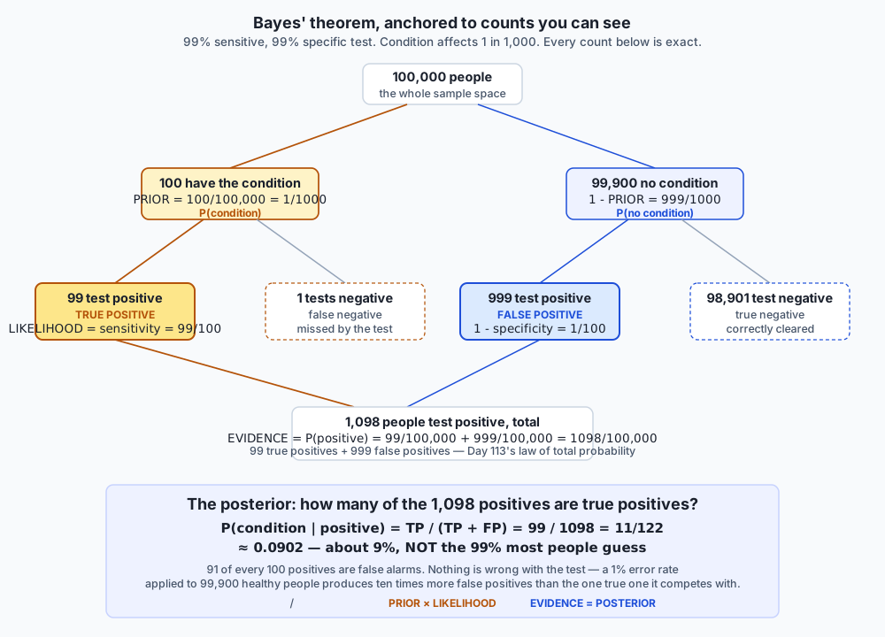
Take 100,000 people at the stated prevalence and rates. 100 have the condition (1 in 1,000, scaled up). Of those 100, the 99%-sensitive test catches 99 — true positives — and misses 1 — a false negative. Of the remaining 99,900 healthy people, the 1% false-positive rate still fires on 999 of them, leaving 98,901 correctly cleared.
| Tests positive | Tests negative | Total | |
|---|---|---|---|
| Has the condition | 99 (true positive) | 1 (false negative) | 100 |
| Does not have it | 999 (false positive) | 98,901 (true negative) | 99,900 |
| Total | 1,098 | 98,902 | 100,000 |
Of the 1,098 people who test positive, only 99 actually have the
condition: 99 / 1098 = 99/1098, identical to the formula’s answer,
because it is the same computation, counted instead of multiplied. This is
exercise 2 of the lab, and its harness asserts the ratio matches the
formula exactly, not approximately — there is no rounding anywhere in
either route, so an exact match is the correct expectation, not a
coincidence.
The odds form
The probability form of Bayes’ theorem is correct, but it buries a useful
fact inside a division. The odds form surfaces it. Convert a
probability to odds with odds = p / (1 - p), and back with p = odds / (1 + odds). Then:
posterior odds = prior odds x likelihood ratiowhere the likelihood ratio for a positive result, often written
LR+, is P(positive | condition) / P(positive | no condition) —
sensitivity over the false-positive rate.
For the opening scenario: prior odds are (1/1000) / (999/1000) = 1/999
— about 1 case for every 999 non-cases. The likelihood ratio is (99/100) / (1/100) = 99 — a positive result is 99 times more likely if you have the
condition than if you don’t. Multiply: posterior odds are (1/999) x 99 = 99/999 = 11/111. Convert back: 11/111 / (1 + 11/111) = 11/122 — the
identical answer, arrived at by multiplication instead of division, and
05_odds_form.py confirms both routes agree exactly.
The odds form earns its place in this lesson for one reason: the likelihood ratio isolates exactly how much a piece of evidence is worth, completely independently of what you believed before you saw it. A likelihood ratio of 99 means “this evidence is 99 times more consistent with the hypothesis than with its negation” — full stop, regardless of the prior. That property is what makes sequential updating, the next section, almost trivial to reason about.
Sequential updating, and the order that does not matter
Suppose two different tests both come back positive: test A, the opening scenario’s 99%/99% test, and test B, a different, less accurate test at 95% sensitivity and 98% specificity. Update with A first, then B — or B first, then A. This lesson’s lab computes both orders explicitly rather than asserting the outcome from algebra alone.
Update with A: prior odds 1/999, likelihood ratio 99, giving posterior
odds 11/111 — a probability of 11/122 ≈ 0.0902, exactly the opening
scenario. Now update again with B: B’s likelihood ratio is (95/100) / (1 - 98/100) = (95/100) / (2/100) = 95/2 = 47.5. Multiply onto the running
odds: (11/111) x (95/2) = 1045/222. Converting back to a probability
gives 1045/1267 ≈ 0.824783 — over 82%.
Reverse the order — B first, then A — and the running odds at the end are
(1/999) x (95/2) x 99, exactly the same three numbers multiplied
together, just grouped differently. 06_sequential_updating.py computes
both orders independently and confirms the final posterior is identical to
the digit: Fraction(1045, 1267) either way. This is not a special
property of Bayes’ theorem. It is a special property of multiplication —
a x b x c equals c x b x a for any real numbers — that Bayes’ theorem
happens to be built from, once it is written in odds form. Each update
multiplies one more likelihood ratio onto a running product, and a product
does not care what order its factors arrived in.
The honest caveat: when “just multiply” quietly assumes something false
Sequential updating’s clean commutativity depends on one assumption that is easy to state and easy to forget: the pieces of evidence must be conditionally independent given the hypothesis. Test A and test B in the previous section are genuinely different tests, run independently, so multiplying their likelihood ratios is the correct move. But now suppose the “two tests” are the same test, run twice on one sample. Two runs of the same assay on the same sample often violate independence badly — a contaminated sample, a bad batch of reagent, or any shared failure mode affects both runs identically, not independently.
Construct this concretely. Use the opening scenario’s test — 99% sensitive, 99% specific — run twice on one sample, and suppose that half the time, both runs are yoked to a single shared outcome (a shared failure mode) rather than drawn independently; the other half of the time, they genuinely are independent. The naive calculation — the one built by squaring the single-run likelihoods, exactly as if the two runs were fully independent — computes:
P(both positive | condition)    = sensitivity^2         = 9801/10000
P(both positive | no condition) = (1-specificity)^2     = 1/10000

naive posterior = 363/400 = 0.9075
The correct calculation accounts for the correlation directly: half the time both runs share one draw at the single-run rate, half the time they are independent as above:
P(both positive | condition)    = (1/2)(99/100) + (1/2)(99/100)^2  = 19701/20000
P(both positive | no condition) = (1/2)(1/100)  + (1/2)(1/100)^2   =   101/20000

correct posterior = 2189/13400 ≈ 0.1634
Both numbers are computed and printed by 07_correlated_tests.py. The
naive calculation reports over 90% confidence. The correct calculation
reports about 16%. The correct one is right, and the naive one is
not just imprecise — it is dramatically overconfident, because it treats
one piece of evidence (the shared failure mode, when it occurs) as if it
were two independent pieces, double-counting it in exactly the same shape
of mistake the addition rule’s naive sum made back on Day 113: counting
something that belongs to only one “bucket” as if it belonged to two.
Multiplying likelihood ratios is the right move only when the evidence
streams really are independent given the hypothesis; two runs of the same
assay on the same sample are a realistic, common case where they are not,
and this lesson would be dishonest to teach sequential updating without
saying so.
Base-rate neglect and the prosecutor’s fallacy
Base-rate neglect, already the villain of the opening scenario, is
worth naming precisely: it is the tendency to weigh how reliable a piece
of evidence is while ignoring how likely the hypothesis was before the
evidence arrived. A 99%-accurate test applied to a condition with a
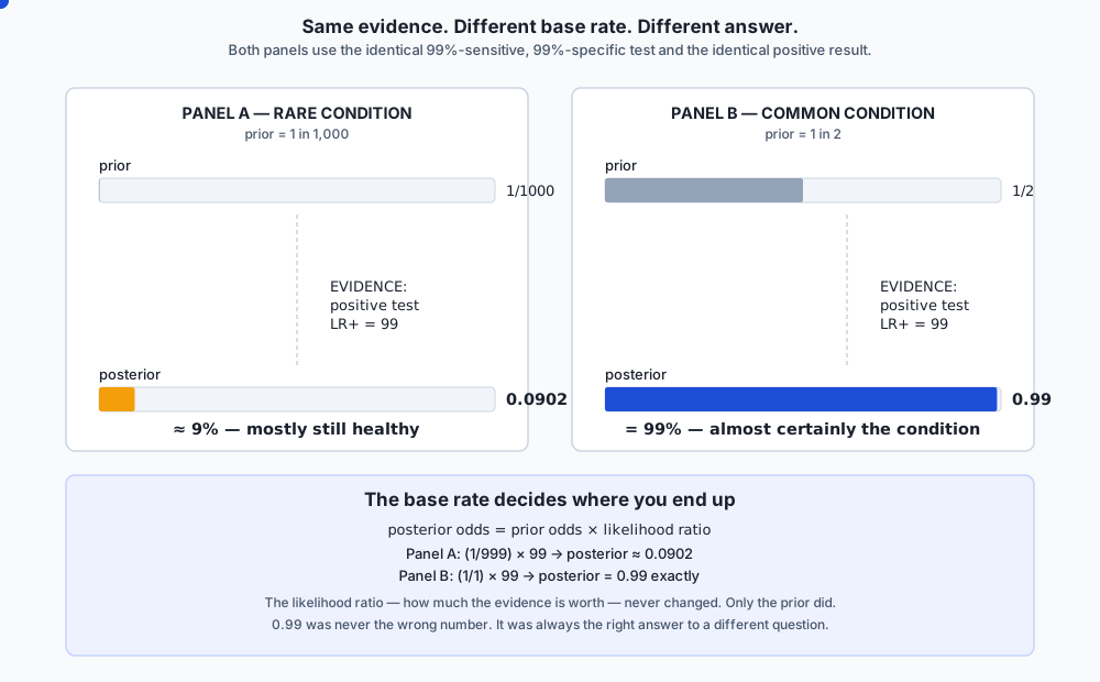
1-in-1,000 base rate produces a posterior near 9%; the same 99%-accurate
test applied to a condition with a 1-in-2 base rate produces a posterior
of exactly 0.99 — the natural number everyone gives for the rare case,
now the genuinely correct answer for a common one. Exercise 4 of the lab
sweeps prevalence from 1-in-100,000 up to 1-in-2 and shows the posterior
climbing monotonically, landing on exactly Fraction(99, 100) at the top
of the sweep. The number 0.99 was never wrong; it was answering a
different question the whole time, one about a much more common
condition.
The prosecutor’s fallacy is base-rate neglect’s courtroom-specific
cousin, and it deserves its own name because the stakes are higher and the
mistake is depressingly common in real trials: treating
P(evidence | innocent) as if it were P(innocent | evidence). Suppose a
piece of forensic evidence — a DNA partial match, say — would occur in
only 1 person in a million who is innocent: P(evidence | innocent) = 1/1,000,000. A prosecutor might argue this means the defendant is
“999,999 times more likely to be guilty than innocent.” That argument
silently assumes the only question that matters is how rare the
evidence is under innocence — it ignores how many innocent people could
plausibly have been tested in the first place, and it ignores the actual
prior probability of guilt before the evidence. In a city of ten million
people, a 1-in-a-million false-match rate still implicates roughly ten
innocent people purely by chance, and without a genuine prior narrowing
the suspect pool well before the DNA evidence, P(evidence | innocent)
being tiny does not make P(innocent | evidence) tiny — it is Bayes’
theorem, not the raw likelihood, that says how the two actually relate,
and the fallacy is skipping straight from one to the other as if they were
interchangeable.
Naive Bayes from scratch
Everything above updates belief about a single hypothesis given a single
event. Naive Bayes applies exactly the same machinery to classify a
document by treating every word in it as a separate piece of evidence,
updated one at a time. “Naive” names one specific, deliberately false
assumption: that every word’s presence is conditionally independent of
every other word’s presence, given the document’s class. That is not
true — word choice is shaped by context and grammar, not independent draws
— and the classifier works well anyway, because ranking P(spam | words)
against P(ham | words) correctly does not require the independence
assumption to be literally true, only for its errors to not systematically
favour the wrong class.
Train on a tiny, hand-made corpus so every count can be checked by hand:
three spam documents ("buy cheap watches now", "cheap replica watches for sale", "buy now limited offer") and three ham documents
("meeting notes for review", "please review the agenda", "schedule the project meeting"). That gives a 17-word vocabulary and, critically,
two words that never cross class lines in training: "watches" never
appears in a ham document, and "review" never appears in a spam
document.
The classifier’s score for a document under a class is P(class) times
the product of P(word | class) over every word — document_score() in
the lab, computed as an exact Fraction. Two things the textbook version
of this idea glosses over, and this lesson does not:
The one-word veto. Without smoothing, P(word | class) for a word
that never appeared in that class’s training data is exactly count / total = 0 / total = 0. Multiply anything by zero and the whole product is zero,
no matter how strongly every other word points the other way. Classify the
held-out document "please review schedule watches" — three words
(please, review, schedule) that are strongly ham-associated, and one
(watches) that is spam-associated — and the unsmoothed classifier’s
score for both classes collapses to exactly zero on this run: review
zeroes out spam’s score (it never appeared in spam training), and
watches zeroes out ham’s score (it never appeared in ham training). With
both classes tied at exactly 0, the classifier’s max() call silently
returns whichever class happens to be listed first — not the class the
evidence actually supports — and this document, correctly classified ham
with smoothing, is misclassified spam without it, purely because of tie-
break order.
Laplace (add-one) smoothing is the fix. Instead of count(word, class) / total_words(class), compute (count(word, class) + alpha) / (total_words(class) + alpha x |vocabulary|) with alpha = 1. Every word
in the vocabulary now gets a small, non-zero probability under every
class, including words never seen in that class’s training data — so no
single absent word can single-handedly decide a classification. With
smoothing, the veto-case document above correctly classifies ham, because
the three ham-associated words’ combined evidence now outweighs the one
spam-associated word’s small, non-zero counter-evidence, rather than being
erased by it. This is exactly the toy version of exercise 8, and it holds
in the reference run: 08_naive_bayes_smoothing.py confirms both clean
documents classify identically smoothed or not, and confirms the veto
document classifies ham with smoothing and misclassifies without it, with
both unsmoothed scores landing at exactly 0.
Log space is the second thing the textbook version glosses over, and
it is not about correctness for this tiny four-word corpus — it is about
what happens at realistic scale. A real document has hundreds of words,
each contributing a per-word probability on the order of a percent or two.
Multiplying several hundred numbers that small, as plain float64, does
not merely lose precision — it can underflow to exactly 0.0.
09_log_space.py demonstrates this directly rather than asserting it:
multiplying 500 factors of 0.01 as a running float64 product reaches
0.0 well before the 500th factor (the printed trace shows it still
finite at 100 factors, already 0.0 by 200), and the true value —
0.01^500 = 10^-1000 — sits about 676 orders of magnitude below
float64’s smallest representable positive number, roughly 5e-324.
Once a document’s plain-product score underflows this way, every class
ties at exactly 0.0 and the classifier again silently returns whichever
class came first — the identical failure mode as the one-word veto, this
time caused by scale rather than by an absent word.
The fix is the same idea Day 110’s vanishing-gradient discussion and Day
46’s floating-point representation both anticipated: work in log space. A
product of small probabilities becomes a sum of their logarithms —
large, negative numbers, but nowhere near float64’s limits. math.log(0.01) ≈ -4.6052, and summing 500 copies of it gives exactly
-2302.5850929940457, computed directly by sum_of_logs() in this
lesson’s lab and confirmed finite. (One correction worth stating plainly:
an earlier draft of this lesson’s brief cited the log-space figure for 500
factors of 0.01 as “about -1151.29” — that number is wrong for this
computation; it is what 500 factors of 0.1 produce instead, or
equivalently 250 factors of 0.01. Every figure in this lesson and its
lab uses the measured, correct value, computed directly by math.log
rather than copied from a draft — when a measurement contradicts a stated
figure, the measurement wins, and this lesson says so rather than quietly
fixing it and moving on.) classify_log_space() performs the identical
classification decision as the plain-product version, but by summing logs
and comparing sums instead of multiplying probabilities and comparing
products — the version a real implementation ships, not the version that
makes the underflow visible for teaching purposes.
An everyday analogy
Think of a detective walking into a scene with a short list of suspects and a rough sense, before finding any clues, of how likely each one is — the prior. Every clue found at the scene is evidence, and the detective’s job is not to ask “how rare is this clue” in isolation, but “how much more consistent is this clue with suspect A than with everyone else” — the likelihood ratio. A fingerprint that only 1 person in a million could produce sounds damning in isolation, but if a million people plausibly passed through that room, the clue alone barely narrows anything down; if only three people had access to the room at all, the same fingerprint is close to conclusive. The clue’s rarity in the abstract is not the question. Its rarity relative to how many suspects it could plausibly implicate is.
Each new clue updates the running odds on every suspect — multiply the running odds by the new clue’s likelihood ratio, exactly as this lesson’s odds form does — and it does not matter what order the clues are examined in, because multiplication does not care about order. But a careful detective asks one more question before combining two clues: are they truly independent evidence, or could one explanation account for both at once? Two witnesses who both say they saw the same car are only two independent pieces of evidence if they did not talk to each other first; if they compared notes before giving statements, their two “independent” accounts are really one piece of evidence, reported twice — exactly exercise 7’s correlated-tests scenario, in courtroom clothing rather than laboratory clothing.
Where the analogy strains: a detective’s prior is usually an informal hunch, hard to pin to an exact number, while this lesson’s examples all start from a stated, numerical prior (a disease’s known prevalence, a spam corpus’s known class balance). That numerical starting point is what makes exact computation possible at all — the detective analogy illustrates the reasoning, but the lab’s every claim is checkable precisely because the priors and likelihoods in it are stated numbers, not hunches.
Examples in practice
The opening scenario, worked completely
Already derived in full above: prior 1/1000, sensitivity and specificity
both 99/100, posterior 99/1098 = 11/122 ≈ 0.0902. Confirmed by the
natural-frequency table (99 true positives against 999 false
positives, out of 1,098 total positives) and by a 2,000,000-person
seeded simulation. On the captured run in this lesson’s lab, with seed
42, the simulation produced 1,978 true positives and 20,069 false
positives among 2,000,000 simulated people, an empirical posterior of
0.089717, landing 0.000447 from the exact 0.090164 — well inside the
three-standard-error tolerance of about 0.005787 at that many positive
results. Three independent methods, three independent confirmations of
the same number, none of them tuned to agree with the others.
The prevalence sweep, and where 0.99 becomes the right answer
| Prevalence | Posterior |
|---|---|
| 1 in 100,000 | 11/11122 ≈ 0.000989 |
| 1 in 10,000 | 1/102 ≈ 0.009804 |
| 1 in 1,000 (the opening scenario) | 11/122 ≈ 0.090164 |
| 1 in 100 | 1/2 = 0.5 |
| 1 in 10 | 11/12 ≈ 0.916667 |
| 1 in 2 | 99/100 = 0.99 exactly |
The posterior climbs strictly with prevalence, and lands on precisely the
naive 0.99 guess once the condition is as common as a coin flip. This is
the clearest possible demonstration of what a base rate does: the exact
same test, the exact same evidence, and a completely different right
answer depending on nothing but how common the condition was to begin
with.
Sequential updating and its correlated-evidence caveat, side by side
Two genuinely different tests (99%/99% and 95%/98%), both positive: 1045 / 1267 ≈ 0.8248, identical regardless of update order. The same test run
twice on one correlated sample: a naive posterior of 363/400 = 0.9075
against a correct, correlation-aware posterior of 2189/13400 ≈ 0.1634 —
both computed in the lab, both printed side by side, with the naive
figure strictly and substantially the higher of the two. Put the two
scenarios next to each other and the lesson is concrete rather than
abstract: genuinely independent evidence combines by simple multiplication
of likelihood ratios; evidence that shares a hidden common cause does not,
and treating it as if it did produces false confidence, not just a
slightly different number.
The Naive Bayes veto case
"please review schedule watches" — three ham-associated words, one
spam-associated word. Smoothed: classified ham, correctly, with every
word’s evidence genuinely weighed. Unsmoothed: both classes’ scores are
exactly 0.0, and the classifier returns whichever class its max() call
happens to see first — spam on this implementation, misclassifying a
document that four out of five of its words support as ham. The gap
between these two outcomes is not a rounding difference; it is the
difference between a classifier that weighs evidence and one that lets a
single absent word silently override everything else.
Implications: security, privacy, performance, scalability, and cost
Security. Fraud-detection and intrusion-detection systems are, at bottom, sequential Bayesian updates: each signal (an unusual login location, a rapid sequence of transactions, a mismatched device fingerprint) has a likelihood ratio, and the running odds accumulate as signals arrive. Treating correlated signals as independent — several alerts that all trace back to one compromised credential, say — inflates confidence exactly the way exercise 7’s correlated tests do, and a system that does not account for shared root causes among its signals will report higher certainty than the evidence actually supports, which is a genuine security risk when that false certainty drives an automated response.
Privacy. A system that reports “94% confidence this is you” based on a biometric or behavioural match is making a posterior probability claim, and that claim is only as trustworthy as its prior — the base rate of legitimate users versus impostors in the population the system actually serves. A system trained or validated against a different, more balanced population than its real deployment will misstate its own confidence in exactly the base-rate-neglect shape this lesson opened with, with direct consequences for how much weight a human reviewer or an automated policy should place on the reported number.
Performance and cost. Every computation in this lesson and its lab —
the opening posterior, the prevalence sweep, the odds-form updates, the
Naive Bayes classifier’s training and inference — is O(1) or, for Naive
Bayes, linear in the number of words in a document and the size of the
vocabulary. None of it is computationally expensive. The expensive
alternative this lesson deliberately does not reach for is full posterior
inference over continuous parameters (Markov Chain Monte Carlo, as PyMC
or Stan perform) — genuinely useful when the question is “what is the
whole distribution of plausible parameter values,” genuinely wasteful when
the question is the single discrete update this lesson answers, which a
few lines of exact arithmetic settle instantly.
Scalability. A production Naive Bayes classifier scales to vocabularies of hundreds of thousands of words and documents of any realistic length — provided it is built in log space. The plain-product version this lesson deliberately builds first is not a smaller-scale variant of the real thing; past a few dozen words, it silently stops working at all, in the specific, demonstrated way exercise 9 shows. Scalability here is not about handling more data faster — it is about the arithmetic remaining correct at the scale the application actually needs, which log space is a hard requirement for, not an optimisation.
The specific cost of getting this wrong. A wrongly-computed posterior looks exactly like a correctly-computed one: it is a number between 0 and 1, it has a plausible number of decimal places, and nothing about its appearance signals the mistake. This lesson’s entire structure — three independent methods for the opening scenario, both orderings for sequential updating, naive against correlation-aware for exercise 7, smoothed against unsmoothed for the classifier — exists because that is the only reliable defence: compute it more than one way and confirm they agree, rather than trusting the first plausible-looking answer.
Alternatives: free, open source, and commercial
Hand-rolled Python with fractions.Fraction — free, standard library,
and what every exact calculation in this lesson and its lab actually uses.
Choose it whenever a posterior needs to be checkable exactly rather than
approximately — every exact number quoted in this lesson (99/1098,
1045/1267, 363/400, and the rest) is a Fraction, comparable for exact
equality, never subject to float rounding. Its limitation is exactly its
strength: Fraction has no notion of continuous distributions and no
built-in inference machinery beyond exact rational arithmetic on
enumerable, discrete probabilities — for anything continuous, this lesson
reaches for the tools below.
numpy.random.default_rng — free and open source (BSD 3-Clause), and
what exercise 3’s 2,000,000-person population simulation actually uses.
Called as rng = np.random.default_rng(seed), then vectorised draws such
as rng.random(n) < prevalence build the whole simulated population in a
handful of array operations rather than a Python-level loop. Choose it
whenever a claim needs an independent, simulation-based check rather than
(or alongside) exact arithmetic — as this lesson’s opening scenario gets
both.
scipy.stats — free and open source (BSD 3-Clause), with commercial
support available through various vendors for organisations running SciPy
in production. Not installed in this environment, and no output from it
is reproduced anywhere in this lesson or its lab; everything said about it
here is drawn from its public documentation rather than from a run.
According to that documentation, scipy.stats provides the named
distributions Day 114 introduced (binomial, Bernoulli, and dozens more),
each with methods for probability mass or density, cumulative distribution
and sampling. Choose it once a Bayesian update needs a distribution of
outcomes rather than a single point estimate — for instance, modelling
sensitivity itself as uncertain (a Beta distribution) rather than as a
fixed, known 99%. That distributional extension is exactly what this
lesson’s single-point updates deliberately stop short of.
scikit-learn’s MultinomialNB — free and open source (BSD 3-Clause).
Not installed in this environment; described from its public
documentation, not run here. MultinomialNB is scikit-learn’s
production Naive Bayes classifier for word-count or frequency features,
called roughly as MultinomialNB(alpha=1.0).fit(X, y) where X is a
document-term count matrix. Its alpha parameter is precisely the Laplace
smoothing constant this lesson’s word_probability() implements by hand —
alpha=1.0 is add-one smoothing, alpha=0.0 reproduces the unsmoothed,
veto-prone version this lesson demonstrates failing. Choose it the moment
a real corpus is large enough that a hand-rolled classifier’s bookkeeping
(vocabulary management, sparse count matrices, log-space internals) stops
being worth reimplementing — which is most real corpora; this lesson’s
four-word toy documents exist purely so the failure modes can be inspected
by hand, not as a template for production code.
PyMC or Stan — both free and open source (PyMC: Apache 2.0; Stan: BSD 3-Clause), with no paid tier for either. Neither is installed in this environment; both are described from their public documentation, not run here. Both are probabilistic programming languages for full posterior inference — given a model with several uncertain parameters, they compute (via Markov Chain Monte Carlo sampling, typically) the entire joint posterior distribution over all of them simultaneously, not a single point update like every calculation in this lesson. Choose PyMC or Stan the moment the question changes from “what is the updated probability of this one hypothesis” to “what is the full distribution of plausible values for several interrelated parameters at once, given all the data” — for instance, jointly inferring a disease’s true prevalence and a test’s true sensitivity and specificity from imperfect field data, rather than treating all three as known constants as this lesson does throughout. That is a meaningfully harder and more general problem than anything in this lesson, and reaching for MCMC machinery to answer today’s single-update questions would be substantial, unnecessary overhead.
The honest summary: for the exact, discrete updates this lesson covers,
fractions.Fraction is free, exact and sufficient — there is no
meaningfully better tool. numpy.random.default_rng is the right default
for a simulation-based check. scipy.stats, MultinomialNB, PyMC and
Stan all become relevant once the problem grows past a single point
update — a full distribution over an uncertain parameter, a large real
corpus, or a joint inference over several interrelated unknowns — and this
lesson names each one honestly as something not run here, not something
approximated.
Comparison with related concepts
Bayes’ theorem and the law of total probability. Already covered in detail above: the law of total probability (Day 113) computes an unconditioned probability by summing conditional probabilities weighted by how likely each condition is. Bayes’ theorem’s denominator is exactly that computation, applied to the event actually observed. They are the same arithmetic, read in opposite directions — Day 113’s urns forward, this lesson’s diagnostic test backward.
The probability form and the odds form. Mathematically equivalent — this lesson proves it directly, computing the opening scenario’s posterior both ways and confirming an exact match. The probability form is more familiar and reads more naturally as “here is the answer.” The odds form is more useful for reasoning, because it isolates the likelihood ratio as a self-contained measure of what a piece of evidence is worth, independent of the prior — which is exactly what makes sequential updating tractable to reason about at all.
Sequential updating and correlated evidence. Sequential updating in odds form is simple multiplication and therefore commutative — order never matters — but that simplicity rests entirely on the evidence streams being conditionally independent given the hypothesis. When they are not (two runs of one assay on one sample, two fraud signals both traceable to one compromised credential), naive multiplication of likelihood ratios overstates confidence, and the correct calculation needs to model the shared cause directly, as exercise 7 does.
Base-rate neglect and the prosecutor’s fallacy. Base-rate neglect is
the general failure — ignoring how common a hypothesis was to begin with.
The prosecutor’s fallacy is the specific instance of confusing
P(evidence | innocent) with P(innocent | evidence), most consequential
in legal reasoning about forensic evidence. Both are corrected by the same
tool: actually applying Bayes’ theorem rather than reasoning about the
likelihood in isolation.
“Naive” in Naive Bayes and independence, from Day 113. Day 113 built a whole table distinguishing genuine independence from mutual exclusivity. Naive Bayes’s “naive” assumption is a specific application of independence — that each word’s presence is conditionally independent of every other word’s, given the document’s class — known in advance to be false (word choice is not independent of context), and used anyway because the classifier’s practical accuracy does not require the independence assumption to be literally true.
When to use it — and when not to
Apply Bayes’ theorem directly whenever you have a prior, a likelihood, and need a posterior for a single, well-defined hypothesis — a diagnostic test result, a single piece of evidence, a single classification decision. The probability form and the odds form are equivalent; use the odds form when you plan to combine several pieces of evidence, since it makes each piece’s contribution explicit and separable.
Check independence before combining evidence. Multiplying likelihood ratios is only correct when the evidence streams are genuinely conditionally independent given the hypothesis. Two readings from the same instrument, two opinions informed by the same underlying data, or two alerts traceable to one root cause are common, realistic violations — model the shared cause directly, as exercise 7 does, rather than assuming independence because the two pieces of evidence arrived through different- sounding channels.
Always ask which conditional probability you actually have.
P(evidence | hypothesis) and P(hypothesis | evidence) are different
numbers, and confusing them — in a diagnostic claim, a legal argument, or a
classifier’s marketing material — is the single most consequential mistake
this lesson addresses.
Smooth a Naive Bayes classifier; never ship the unsmoothed version.
The one-word veto is not a rare edge case at realistic vocabulary sizes —
any sufficiently large training corpus will have words that are absent
from at least one class, and any sufficiently varied set of held-out
documents will eventually contain one. Laplace smoothing (alpha >= 1,
scikit-learn’s MultinomialNB(alpha=...)) is close to free and prevents
an entire, silent failure mode.
Build a real classifier in log space, not as a literal product. The
plain-product version exists in this lesson to make the underflow failure
visible for teaching purposes. A real implementation — hand-rolled or via
MultinomialNB — always works in log space or an equivalent numerically
stable formulation; nothing about production Naive Bayes should ever
multiply raw probabilities together across a realistic document.
Reach for scipy.stats, PyMC, or Stan only once the question grows
past a single point update — modelling a parameter itself as uncertain, or
inferring several interrelated unknowns jointly from data. Using MCMC
machinery to answer a single discrete update, of the kind every example in
this lesson works through with a few lines of exact arithmetic, is
substantial unneeded overhead.
Knowledge check
Eight questions accompany this lesson, covering the opening scenario’s exact posterior and why the naive 99% answer is wrong, the natural- frequencies reframing as the same arithmetic made obvious, why the denominator of Bayes’ theorem is Day 113’s law of total probability, the odds form and why order does not matter for genuinely independent evidence, the correlated-tests case where naive multiplication overstates confidence, the distinction between base-rate neglect and the prosecutor’s fallacy, the one-word veto that Laplace smoothing prevents, and why a real classifier is built in log space.
Two are worth attempting before reading anything else: the one asking for the opening scenario’s true posterior, and the one asking what specifically goes wrong when two correlated pieces of evidence are treated as independent. Those are the two facts the rest of the lesson is built on.
Hands-on exercise
The lab is “Bayes You Can Trust,” and its design principle is the one
Days 113 and 114 both used: compute everything two independent ways and
assert they agree — exact rational arithmetic with fractions.Fraction
wherever the answer is rational, seeded simulation otherwise, with
tolerances derived from the standard error of a proportion.
cd labs/sections/math-statistics-and-data/day-115-bayes-theorem
python3 -m venv .venv
.venv/bin/pip install -r requirements/requirements.txt
Nine exercises, in order: the opening posterior, derived exactly; the same
arithmetic as a natural-frequencies table; a two-million-person seeded
simulation; the prevalence sweep, ending at exactly 0.99; the odds form;
sequential updating in both orders; correlated tests and the honest
overstated-confidence case; a from-scratch Naive Bayes classifier with
Laplace smoothing and the one-word veto; and the log-space arithmetic that
makes the classifier work at realistic scale.
Check yourself as you go:
.venv/bin/pytest starter -qUnattempted work is reported as skipped, never as failed. Wrong work fails with your answer printed beside the correct one.
Expected output
An untouched checkout:
2 passed, 38 skippedA finished one:
40 passedThe full harness ends with:
53 checks, 0 failure(s).and exits 0. Along the way, the opening posterior, derived term by term:
P(condition | positive) = 99/1098 = 11/122
                         = 0.090164  ~ 0.0902
and the naive-versus-correlated gap from exercise 7:
  naive (assumes independence):  0.9075  (90.8% confident)
  correct (accounts for the shared failure mode): 0.1634  (16.3% confident)
Validate your work
bash tests/run_tests.sh; echo "exit=$?"prints53 checks, 0 failure(s).andexit=0..venv/bin/pytest examples -q -p no:cacheproviderprints71 passed..venv/bin/pytest starter -q -p no:cacheproviderprints40 passedwhen you are finished.- Each of the nine reference scripts ends with
every assertion held. - Your
posterior()function returns aFraction, never afloat— an assertion comparing it againstFraction(99, 1098)must pass exactly, not approximately.
Troubleshooting
ModuleNotFoundError on bayes, simulate or naive_bayes means you ran
a reference script from the lab directory rather than from inside
examples/; they import their neighbours from beside themselves.
Tests that keep skipping after you have written code usually mean a
leftover raise NotImplementedError survived below your implementation.
A posterior() result that comes out close to 0.99 instead of 0.09
almost always means the denominator was never actually the full law of
total probability sum — check that both the sick-population term and the
healthy-population term are present and added together, not just the
first.
likelihood_ratio() giving exactly 1 means it was computed as
sensitivity / specificity instead of sensitivity / (1 - specificity) —
a likelihood ratio of 1 claims the evidence is worth nothing, which
should look wrong on sight for a diagnostic test.
troubleshooting.md covers all of these in full, along with why the
harness clears bytecode caches at the start of its run.
Common mistakes
- Returning the sensitivity, or something close to it, from
posterior(). Reproduces the exact base-rate-neglect error this lesson opens with; the fix is confirming the full evidence term includes both the sick and the healthy population’s contributions. - Computing the likelihood ratio with the wrong denominator. It is
sensitivity / (1 - specificity), the false-positive rate — notsensitivity / specificity. - Assuming sequential updating “should” depend on order. It does not, for genuinely independent evidence, because it is built from commutative multiplication in odds space; the lab’s exercise 6 computes both orders explicitly to prove it rather than merely asserting it.
- Treating exercise 7’s naive and correlated posteriors as interchangeable. The naive one overstates confidence; the lab asserts the naive result is strictly higher, never merely different.
- Believing Laplace smoothing “fixes” the independence assumption. It does not — it only prevents one specific failure mode, a single absent word vetoing an entire classification. The independence assumption stays false either way; the classifier is useful despite that, not because smoothing corrected it.
- Building the Naive Bayes classifier in log space from the start and
never observing the underflow. Not wrong for a working classifier, but
it skips watching
multiply_probabilities()actually reach exactly0.0, which is the whole point of exercise 9.
Practice assignment
Extend today’s tools to a problem this lesson did not work through.
- A three-test sequential update. Add a third test with its own sensitivity and specificity to exercise 6’s scenario, confirm the posterior is identical across all six possible orderings of the three tests, and find the order-invariant quantity directly — the product of all three likelihood ratios — rather than checking every permutation by brute force.
- Sweep the correlation weight continuously. Vary
correlation_weightin exercise 7’s scenario from 0 to 1 in small steps, and confirm the correlation-aware posterior is a strictly decreasing function of it: full independence (0) reproduces the naive answer as an upper bound, and full correlation (1) collapses to a single test’s posterior as a lower bound, since two fully-correlated results carry no more evidence than one. - The prosecutor’s fallacy, made concrete. Pick a stated prior
probability of guilt (before any forensic evidence) and a stated
P(evidence | innocent), and computeP(innocent | evidence)properly with Bayes’ theorem rather than treating the two conditional probabilities as interchangeable. Write one paragraph on how large the gap between the two numbers is, and why. - Add a third class to the Naive Bayes classifier. Introduce a
“newsletter” class alongside spam and ham with its own small corpus,
and confirm
classify_log_space()still picks correctly among three classes — the log-space argmax generalises to any number of classes with no changes beyond iterating over more of them. - Measure calibration on invented predictions. Generate a set of invented model-confidence values alongside invented true/false outcomes where the model is deliberately overconfident, bucket the confidences, and compute the empirical accuracy within each bucket — a direct, hands-on version of the calibration idea in this lesson’s AI thread below.
Extension challenge
Three, in increasing order of difficulty.
Infer a test’s unknown sensitivity from data. Suppose, instead of
being told the test is 99% sensitive, you only observe outcomes from n
known-sick patients who were tested. Using only fractions.Fraction and
enumeration over a discrete grid of candidate sensitivities (no scipy),
build a posterior distribution over the candidate sensitivities given the
observed outcomes, and find the value with the highest posterior
probability. Compare it to simply using the observed proportion directly,
and describe in your own words what the Bayesian approach adds when n
is small.
Build a full contingency-table simulator and recover every rate from
counts alone. Simulate a population as exercise 3 does, but this time
pretend you do NOT know the true sensitivity, specificity or prevalence —
only the four contingency-table counts (TP, FP, TN, FN) from a simulated
run. Recover estimates of sensitivity, specificity and prevalence from
those counts alone, propagate them back through posterior(), and confirm
the recovered posterior is close to the one computed from the true,
originally-specified rates. This is the practical shape of validating a
real diagnostic test or classifier against a labelled dataset.
Describe, without running it, what a full PyMC posterior would add. Using only the PyMC documentation (do not attempt to install or run PyMC for this exercise, and say so explicitly in your write-up), describe how a PyMC model would treat the opening scenario’s sensitivity, specificity and prevalence as themselves uncertain — each with its own prior distribution — rather than as known constants, and produce a full posterior distribution over the disease-given-positive probability rather than the single point value this lesson computes throughout. Explain in your own words what information that fuller answer carries that today’s point estimate does not, and be explicit that this is a description of the tool’s documented purpose, not a report of anything actually run.
The AI thread. Naive Bayes was the first spam filter that actually
worked at scale, in the late 1990s and early 2000s, and the shape of it
survives everywhere a modern system outputs a probability: a language
model’s stated confidence, a content-moderation classifier’s toxicity
score, a fraud model’s risk number. But the sharper point this lesson
leaves you with is not historical. A classifier’s output is a
posterior, and a posterior is only as trustworthy as the prior that
produced it. A model trained and validated on a class-balanced dataset —
50% spam, 50% ham; 50% fraud, 50% legitimate — and then deployed against a
real population where the positive class is rare will reproduce the
opening scenario’s exact failure at scale: a headline accuracy number that
sounds impressive, and a real-world positive-predictive-value that is
nowhere near it, for exactly the reason 99/1098 is nowhere near 0.99.
Calibration — checking whether a model’s stated confidence matches its actual accuracy, bucket by bucket — is the name of the fix, and it is, at bottom, exactly the conditioning-as-restriction move Day 113 introduced: restrict to the rows where the model said “90% confident,” and ask what fraction of those rows were actually correct. If that measured fraction is not close to 90%, the model’s stated probabilities are wrong in a specific, measurable, and — now that you have this lesson’s tools — fixable way. The gap between a model’s stated confidence and its measured accuracy is not a mysterious property of large neural networks; it is base-rate neglect, at scale, checkable with the same arithmetic that resolved a 370-year-old question about medical tests.
Quiz
Q1. A test is 99% sensitive and 99% specific. The condition affects 1 person in 1,000. You test positive. What is the true probability you have the condition?
- Exactly 50%, since the outcome is now genuinely uncertain
- About 9% -- close to 99/1098 -- because the 1% false-positive rate applied to the much larger healthy population produces more false positives than the tiny sick population can supply true positives
- It cannot be determined without knowing the total population size
- About 99%, matching the test's stated accuracy
Show answer
Answer: B. About 9% -- close to 99/1098 -- because the 1% false-positive rate applied to the much larger healthy population produces more false positives than the tiny sick population can supply true positives
Out of 100,000 people at this prevalence, 100 have the condition and 99,900 do not. The test catches 99 of the 100 sick people (true positives) but also fires on 999 of the 99,900 healthy people (false positives, from the 1% false-positive rate). Among the 1,098 people who test positive, only 99 actually have the condition: 99/1098, about 9.02%. The test's "99% accuracy" describes how it behaves given the true condition status -- it says nothing on its own about how common that condition was to begin with, which is exactly the base rate Bayes' theorem forces into the calculation.
Q2. The denominator of Bayes' theorem, P(evidence), is computed as P(condition) x P(positive|condition) + P(no condition) x P(positive|no condition). What is this expression, in terms of concepts from Day 113?
- It is the addition rule, applied to two overlapping events
- It is a brand new rule specific to Bayes' theorem, unrelated to anything in Day 113
- It is exactly the law of total probability, applied to the partition {condition, no condition}, with "positive" as the event being summed over
- It is the complement rule, applied to the event "no condition"
Show answer
Answer: C. It is exactly the law of total probability, applied to the partition {condition, no condition}, with "positive" as the event being summed over
The law of total probability from Day 113 states P(A) = sum over i of P(piece_i) x P(A | piece_i), for any partition of the sample space. Here the partition is {condition, no condition} and A is "tests positive" -- exactly the same structural computation Day 113 worked across two urns of different composition. Bayes' theorem's denominator is not a new idea; it is that exact rule, arrived at from the opposite direction: instead of asking the overall chance of the event across the partition, Bayes' theorem asks which piece of the partition the observed event most likely came from.
Q3. Two different tests both come back positive: test A (99% sensitive, 99% specific) and test B (95% sensitive, 98% specific). Updated sequentially in odds form, does the order (A then B, or B then A) change the final posterior?
- Yes -- the test performed second always carries more weight than the test performed first
- It depends on which test has the higher sensitivity
- The orders differ, but only by a negligible rounding amount
- No -- both orders give the identical posterior, because each update multiplies the running odds by a likelihood ratio, and multiplication is commutative
Show answer
Answer: D. No -- both orders give the identical posterior, because each update multiplies the running odds by a likelihood ratio, and multiplication is commutative
In odds form, each update multiplies the running odds by one more likelihood ratio: posterior_odds = prior_odds x LR_A x LR_B (or LR_B x LR_A). Since a x b always equals b x a for real numbers, the final product -- and therefore the final posterior -- is identical regardless of the order the two factors are applied in. This is not a special property of Bayes' theorem; it is a property of multiplication that Bayes' theorem, written in odds form, happens to be built from. The lesson's lab computes both orders explicitly and confirms an identical Fraction result to the digit, rather than only asserting the algebra.
Q4. The same diagnostic test is run twice on ONE sample. Half the time, both runs share a single failure mode (a contaminated sample) and give the same result regardless of the true condition; the other half, the two runs are genuinely independent. Why does calculating the posterior as if the two runs were fully independent (squaring the single-run likelihoods) produce a WRONG answer?
- It silently assumes the two runs are conditionally independent given the hypothesis, which is false here, and it overstates confidence by treating one shared piece of evidence as if it were two separate pieces
- It produces the wrong answer because two positive results are always weaker evidence than one
- It does not -- squaring the likelihoods is correct in any two-test scenario
- It produces the wrong answer only because the specific numbers chosen happen to be unusual
Show answer
Answer: A. It silently assumes the two runs are conditionally independent given the hypothesis, which is false here, and it overstates confidence by treating one shared piece of evidence as if it were two separate pieces
Multiplying likelihood ratios (or squaring a single likelihood, for two identical tests) is only valid when the pieces of evidence are conditionally independent given the hypothesis. Here they are not: half the time, a shared failure mode makes the two runs report the same outcome regardless of the true condition, so they are really one piece of evidence, reported twice. The naive calculation reports a posterior of 363/400 = 0.9075, while the correct, correlation-aware calculation gives about 0.1634 -- the naive answer is not just different, it is substantially overconfident, exactly the same shape of error as double-counting an overlap in Day 113's addition rule.
Q5. A prosecutor argues that because a piece of forensic evidence would occur in only 1 innocent person in a million, the defendant is "999,999 times more likely to be guilty than innocent." What is wrong with this argument?
- The argument is wrong only because forensic evidence is inherently unreliable
- The argument is correct, but only if the defendant had no prior connection to the case at all
- It confuses P(evidence | innocent), which is genuinely small, with P(innocent | evidence), which depends on the prior probability of guilt and how many people could plausibly have been tested -- treating a small P(evidence|innocent) as automatically making P(innocent|evidence) small is the prosecutor's fallacy
- Nothing is wrong with it; the reasoning is mathematically sound
Show answer
Answer: C. It confuses P(evidence | innocent), which is genuinely small, with P(innocent | evidence), which depends on the prior probability of guilt and how many people could plausibly have been tested -- treating a small P(evidence|innocent) as automatically making P(innocent|evidence) small is the prosecutor's fallacy
This is the prosecutor's fallacy: treating P(evidence | innocent) as if it were interchangeable with P(innocent | evidence). Bayes' theorem shows these can be very different numbers -- in a city of ten million people, a 1-in-a-million false-match rate still implicates roughly ten innocent people by chance alone, and without a genuine prior narrowing the suspect pool before the forensic evidence, a tiny P(evidence|innocent) does not by itself make P(innocent|evidence) tiny. The correct computation needs the prior probability of guilt and the actual pool of people who could plausibly have produced the evidence, not just the evidence's rarity in isolation.
Q6. A tiny Naive Bayes spam classifier is trained so that the word "watches" never appears in any ham training document. A held-out document contains three strongly ham-associated words and the word "watches". What happens WITHOUT Laplace smoothing (alpha=0)?
- The classifier correctly weighs all four words and classifies the document ham
- P(watches | ham) is exactly 0, so multiplying it into ham's score makes ham's entire probability exactly 0 regardless of the other three words -- a single absent word vetoes all the evidence that would otherwise favour ham
- The classifier ignores "watches" entirely since it has zero probability, and classifies based on the remaining three words
- Laplace smoothing has no effect on this scenario either way
Show answer
Answer: B. P(watches | ham) is exactly 0, so multiplying it into ham's score makes ham's entire probability exactly 0 regardless of the other three words -- a single absent word vetoes all the evidence that would otherwise favour ham
Without smoothing, P(word | class) for a word that never appeared in that class's training data is exactly count/total = 0/total = 0. Multiplying anything by zero gives zero, so a single unseen word can override however much genuine evidence the other words carry. In the lesson's lab, this document's unsmoothed score for BOTH classes actually reaches exactly 0.0 (a second word, "review", is similarly absent from spam training), and the classifier silently returns whichever class happens to be checked first -- not the class the evidence supports. Laplace smoothing (alpha=1) gives every word in the vocabulary a small nonzero probability under every class specifically to prevent this veto.
Q7. A real Naive Bayes classifier is built to sum LOG probabilities rather than multiply raw probabilities together. Why is this not optional at realistic document lengths?
- Log space is only needed when using a GPU, not on a CPU
- Multiplying probabilities is actually faster, so log space is a tradeoff of speed for a purely cosmetic benefit
- Summing logs is merely a stylistic convention with no practical effect
- A product of several hundred small per-word probabilities can underflow to EXACTLY 0.0 in float64, at which point every class ties and the classifier silently returns whichever class came first -- summing logs turns the product into a sum, which stays finite
Show answer
Answer: D. A product of several hundred small per-word probabilities can underflow to EXACTLY 0.0 in float64, at which point every class ties and the classifier silently returns whichever class came first -- summing logs turns the product into a sum, which stays finite
A document with several hundred words, each contributing a per-word probability on the order of a percent or two, is exactly the shape of a product that underflows: multiplying 500 factors of 0.01 as plain float64 reaches EXACTLY 0.0 well before the 500th factor, because the true value (10^-1000) sits roughly 676 orders of magnitude below float64's smallest representable positive number (about 5e-324). Once that happens, every class's score ties at 0.0 and the classifier silently picks whichever class it checks first, regardless of the evidence -- the identical failure mode as the one-word veto, caused by scale instead of an absent word. Summing the corresponding logs instead (500 x ln(0.01) = -2302.585..., computed and confirmed finite) avoids the underflow entirely.
Q8. The word "naive" in Naive Bayes names a specific assumption: that every word in a document is conditionally independent of every other word, given the document's class. Why does the classifier still work well despite this assumption being false?
- Ranking P(spam | words) against P(ham | words) correctly does not require the independence assumption to be literally true -- only for its errors to not systematically favour the wrong class, which holds often enough in practice for the classifier to be useful
- The assumption is not actually false; word choice really is independent of context
- The classifier only works on very short documents where independence happens to hold exactly
- Smoothing corrects the independence assumption, making it effectively true
Show answer
Answer: A. Ranking P(spam | words) against P(ham | words) correctly does not require the independence assumption to be literally true -- only for its errors to not systematically favour the wrong class, which holds often enough in practice for the classifier to be useful
Word choice is genuinely shaped by grammar and context, so the conditional-independence assumption is known to be false. But Naive Bayes only needs to get the RELATIVE ordering right -- which class's score is higher -- not the individual probabilities exactly right. As long as the independence assumption's errors do not systematically push the ranking toward the wrong class, the classifier's decisions stay accurate even though its literal probability estimates are not calibrated. Smoothing (option 3) fixes a completely separate problem -- the one-word veto -- and does nothing to make the independence assumption itself true.
Glossary
- Bayes' theorem
- The identity P(hypothesis | evidence) = P(evidence | hypothesis) x P(hypothesis) / P(evidence), derived in two lines from the definition of conditional probability. It converts a likelihood -- how probable the evidence is under a hypothesis -- into a posterior -- how probable the hypothesis is given the evidence -- correctly weighting the prior probability of the hypothesis along the way.
- Prior
- P(hypothesis), what you believed about a hypothesis before seeing the evidence currently under consideration. In the opening scenario, the prior is the disease prevalence, 1/1000, before any test result is known.
- Likelihood
- P(evidence | hypothesis), how probable the observed evidence is, assuming the hypothesis is true. In the opening scenario, the likelihood of a positive test given the condition is the sensitivity, 99/100.
- Evidence (marginal likelihood)
- P(evidence), the overall probability of the observed evidence across every possible hypothesis, computed as the denominator of Bayes' theorem. This quantity is exactly Day 113's law of total probability applied to the partition of hypotheses and the event that was observed.
- Posterior
- P(hypothesis | evidence), the updated probability of the hypothesis after the evidence is taken into account -- what Bayes' theorem solves for. In the opening scenario, the posterior is P(condition | positive test) = 99/1098, about 9.02%.
- Base-rate neglect
- The tendency to weigh how reliable a piece of evidence is (a test's stated accuracy) while ignoring how common the hypothesis was to begin with (the base rate, or prior). It is the mechanism behind the opening scenario's misconception: focusing on 99% accuracy while ignoring the 1-in-1,000 prevalence.
- Prosecutor's fallacy
- The specific, legally consequential instance of confusing P(evidence | innocent) with P(innocent | evidence). A small P(evidence | innocent) does not by itself imply a small P(innocent | evidence); the correct relationship between the two requires the prior probability of guilt and the size of the pool of people who could plausibly have produced the evidence, which is exactly what Bayes' theorem supplies and the fallacy skips.
- Odds form
- Bayes' theorem restated as posterior odds = prior odds x likelihood ratio, where odds = p / (1 - p). Mathematically equivalent to the probability form, but useful because the likelihood ratio isolates exactly how much a piece of evidence is worth, independent of the prior.
- Likelihood ratio
- For a positive result, LR+ = P(positive | hypothesis) / P(positive | not hypothesis) -- sensitivity divided by the false-positive rate. A likelihood ratio greater than 1 means the evidence favours the hypothesis; a likelihood ratio of exactly 1 means the evidence is worthless for distinguishing the hypothesis from its negation.
- Sequential updating
- Applying Bayes' theorem (in odds form, one likelihood ratio at a time) across multiple pieces of evidence in succession. The order the evidence arrives in does not affect the final posterior, because each update multiplies the running odds by a factor, and multiplication is commutative.
- Conditional independence
- Two pieces of evidence are conditionally independent given a hypothesis when knowing one occurred, given the hypothesis, tells you nothing about whether the other occurred. Sequential updating by multiplying likelihood ratios is only valid when this holds; two runs of the same assay on one sample, sharing a failure mode, are a realistic case where it does not.
- Naive Bayes
- A classifier that applies Bayes' theorem to a document by treating every word as a separate, conditionally independent piece of evidence given the document's class -- an assumption known to be false (word choice is not independent of context) that the classifier remains useful despite, because it only needs the relative class ranking to be correct, not the individual probabilities.
- Laplace (add-alpha) smoothing
- Computing P(word | class) as (count(word, class) + alpha) / (total_words(class) + alpha x vocabulary_size) rather than the raw count ratio. With alpha=1, every word in the vocabulary receives a small nonzero probability under every class, preventing a single word absent from a class's training data from forcing that class's entire probability to exactly zero.
- The one-word veto
- The failure mode Laplace smoothing exists to prevent: without smoothing, a single word with zero training-count in a class gives that class a probability of exactly 0, and multiplying by zero erases every other word's evidence for that class, regardless of how strongly the rest of the document points toward it.
- Log-space underflow
- The failure that occurs when multiplying many small probabilities together as plain float64 numbers: the true product can be far smaller than float64's smallest representable positive value (about 5e-324), and the computed result becomes exactly 0.0. Multiplying 500 factors of 0.01 demonstrates this directly. The fix is summing the logarithms of the factors instead, which stays finite.
- Calibration
- Checking whether a model's stated confidence matches its actual accuracy, typically by bucketing predictions by their stated probability and measuring the empirical accuracy within each bucket -- a direct application of conditioning as restriction. A model trained on a balanced dataset and deployed against a rare-positive-class population will typically be poorly calibrated, in the same shape as the opening scenario's base-rate failure.
Sources and further reading
- fractions — Rational numbers — Python Software Foundation (accessed 2026-08-17)
- Random Generator — NumPy documentation — NumPy Developers (accessed 2026-08-17)
- scipy.stats — SciPy documentation — SciPy Developers (accessed 2026-08-17)
- Naive Bayes — scikit-learn documentation — scikit-learn Developers (accessed 2026-08-17)
- Introduction to Probability — Dartmouth College (accessed 2026-08-17)
Kept in this browser, no account needed. Your progress page turns the whole record into one link you can bookmark or open on another device.