Math, Statistics, and Data › Probability and Statistics › Day 117
Day 117: Sampling and the Central Limit Theorem

After this lesson you will be able to explain why a sample statistic has its own distribution, and compute how much to trust it. You will build the sampling distribution of the mean by literally repeating a sampling experiment thousands of times, watch its own mean settle near the population mean and its own spread settle near sigma/sqrt(n), and measure the sqrt(n) law directly: quadrupling the sample size from 10 to 40 to 160 to 640 roughly halves the standard error at each step, ratios of 1.985, 1.991 and 2.011 against a predicted 2.0. You will demonstrate the central limit theorem from a population shaped nothing like a bell curve, watching the skewness of the sampling distribution of the mean fall monotonically from 1.42 at n=2 to 0.11 at n=320. You will then meet the two honest halves of this topic most treatments skip. First, where the theorem actually fails: the Cauchy distribution has no defined mean or variance, and its sample mean is itself Cauchy distributed for every n -- measured directly, an Exponential population's sample mean tightens by 9.85x from n=10 to n=1,000 while a Cauchy population's sample mean does not tighten at all, ratio 1.02. Second, that sampling bias is not sampling error and n does not fix it: a sampler restricted to the upper half of a population keeps a completely flat error (2.0712 versus 2.0722) across a hundredfold growth in n, while an honest sampler's error shrinks by 10.28x over the same range -- a confidently precise wrong answer is what bias looks like from the inside. You will build the bootstrap completely from scratch, checking it against a known formula for the mean (within about 1%) and applying the identical code to the median, where no formula exists, checked instead against genuinely fresh samples. You will measure how quietly dependence between observations makes the textbook standard-error formula understate the truth by more than a factor of two. And you will compute, from the binomial standard-error formula, that a model scoring 91.4% on a 500-example test beating another by 0.3 points has demonstrated almost nothing -- the gap sits at 0.24 standard errors, well inside noise.
Hands-on lab for this lesson
Lab files on GitHub: https://github.com/ai-roadmap-365/ai-roadmap-365.github.io/tree/main/labs/sections/math-statistics-and-data/day-117-sampling-and-the-central-limit-theorem
- Get the hands-on files. Clone the labs repository once (you can reuse this clone for every lesson). This works on macOS, Linux, and Windows (PowerShell or WSL):
git clone https://github.com/ai-roadmap-365/ai-roadmap-365.github.io.git cd ai-roadmap-365.github.io - Open this lesson's lab. Move into the directory for this specific day. Every lab lives at the same predictable path — section / subsection / week / day:
cd labs/sections/math-statistics-and-data/day-117-sampling-and-the-central-limit-theorem - Read the lab guide. Open `README.md` in that directory. It lists the exact commands, what each does, the expected output, and how to check your work — read it before running anything.
- Run it and check your work. Follow the README's "How to run" section: run the example first to see the finished result, then complete the numbered exercises in `starter/`, then run the tests. The tests pass (exit 0) only when your work is correct.
bash tests/run_tests.sh # or the test command named in the lab README
You can also open the lab as a local page (works offline, shows the file tree and expected output).
Learning objectives
By the end of this lesson you will be able to:
- Explain why a sample statistic (a mean, a proportion, a median) is itself a random variable with its own sampling distribution, its own mean, and its own spread
- State and demonstrate the sqrt(n) law: quadrupling the sample size roughly halves the standard error, and derive why the naive expectation of halving from doubling the data is wrong
- Demonstrate the central limit theorem numerically by measuring the skewness of a sampling distribution of the mean fall toward zero as n grows, starting from a population that is heavily skewed, discrete, or bimodal
- State the Cauchy distribution's counterexample precisely -- the mean of n Cauchy draws is itself Cauchy distributed with the same spread for every n -- and explain why the central limit theorem's finite-variance condition is a real constraint rather than decoration
- Distinguish sampling bias from sampling error, explain why bias does not shrink with more data while error does, and recognize a confidently precise wrong answer as the signature of a biased sampling frame
- Distinguish the law of large numbers (convergence) from the central limit theorem (rate and shape), a distinction routinely conflated
- Build the bootstrap from scratch -- resample with replacement, recompute a statistic, read its standard error off the spread -- and apply it to a statistic with no closed-form standard error
- Demonstrate that dependence between observations makes the naive standard-error formula understate the truth, and explain why this failure mode is more dangerous in practice than an honest formula being merely imprecise
- Compute the standard error of a model-evaluation accuracy from the binomial formula and use it to judge whether a reported improvement is real or noise
- Use numpy.random.default_rng(seed), passed explicitly into every sampling function, and explain why an internally reseeded generator silently breaks both reproducibility and independence between calls
Prerequisites
- Day 113 -- probability rules and the observation that Monte Carlo error shrinks as 1/sqrt(n), named properly today
- Day 114 -- random variables, expectation, variance, the named distributions, and inverse-CDF sampling with numpy.random.Generator
- Day 116 -- descriptive statistics, the n-1 bias correction, and the bootstrap's general shape, applied here to a specific standard-error question
- Comfort with NumPy arrays and basic vectorised operations
- Days 71-74 -- running pytest and reading its skip-versus-fail output
Why this matters
Somebody on your team measures average session length across 30 users this week. They get 42 seconds. They write it in a slide as the number: “average session length is 42 seconds.” Next week, curious, they draw another sample of 30 users from the exact same underlying population — same product, same traffic, same everything — and measure again. They get 51 seconds.
Nobody made a mistake. Nothing changed about the product between the two measurements. The measurement process itself did exactly what it was supposed to do, twice, and produced two different numbers.
This is the single most common quantitative mistake in software and in AI practice, and it is not a mistake of arithmetic. It is a mistake of framing: treating a sample statistic as if it were the truth, rather than as one draw from a distribution of possible answers the sampling process could have produced. A sample mean is not “the average.” It is an estimate of the average, and estimates have their own spread — their own distribution — exactly the way the underlying data does.
Once you see this, you cannot unsee it, and it changes how you read almost every number a data pipeline or a model evaluation hands you. “Model A scored 91.4% and Model B scored 91.1% on the test set” is not a report that A is better. It is a report of two draws from two sampling distributions, and whether that 0.3-point gap means anything at all depends entirely on how wide those distributions are — a question this lesson gives you the tools to answer with an actual number, not a shrug.
Here is the through-line for the whole day, worth holding onto from the first paragraph to the last: the central limit theorem is the reason a sample can tell you anything about a population at all, and the standard error is the price you pay for asking. Day 113 measured that price without naming it — a Monte Carlo estimate’s error fell as 1/sqrt(n), and the lab measured roughly a 23.5x improvement in error going from 100 to 100,000 samples, close to the sqrt(1000) ≈ 31.6x a 1/sqrt(n) law predicts. Today you learn why that law is 1/sqrt(n) and not something else, what has to be true for it to hold, and — just as importantly — two full sections on where it quietly stops holding, because the conditions are not decoration.
For an AI practitioner specifically, this is not optional background. Every accuracy figure, every win rate, every A/B test result you will ever read about a model is a sample statistic computed on a finite test set, and it carries a standard error whether or not anyone reports one. An accuracy of 91.4% measured on 500 held-out examples has a standard error of about 1.25 percentage points — this lesson computes that number from the same binomial formula a coin flip obeys — which means a model that beats another by 0.3 points on that set has demonstrated close to nothing. Leaderboards are full of exactly this mistake.
The idea in plain language
Here is the reframe in one sentence: a statistic — a mean, a proportion, a median, anything you compute from a sample — is itself a random variable, with its own distribution, its own mean, and its own spread.
Day 114 built random variables as functions from outcomes to numbers. A sample mean is a random variable in exactly that sense: its “outcome” is which 30 users happened to land in your sample, and its “number” is the mean session length of those particular 30 people. Draw a different set of 30 users and you get a different outcome, and therefore a different number. The distribution of that number, across every possible sample you could have drawn, is called the sampling distribution of the mean.
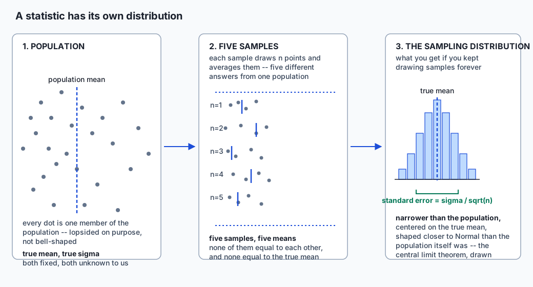
Follow the picture left to right, because it is the whole conceptual leap of the day compressed into one image. On the left is the population — every user who could ever open the app, some of them fast, some slow, the whole messy shape. In the middle, five different samples are drawn from that population, each one a handful of dots pulled out at random, and each sample has its own mean — five short ticks, none of them identical, none of them exactly equal to the population’s true mean. On the right is the object this lesson is actually about: not any one sample, and not the population, but the distribution you would get if you kept drawing samples and kept recording their means, forever. That distribution is narrower than the population itself — averaging cancels out some of the individual noise — and its width has a name: the standard error.
Two results make this reframe usable rather than merely humbling.
The standard error is sigma / sqrt(n). sigma is the population’s own spread; n is your sample size. The sqrt(n) in the denominator is the entire economics of measurement, and it is worth sitting with because it is stingier than intuition expects: to cut your standard error in half, you do not need twice the data — you need four times the data. To cut it to a tenth, you need a hundred times the data. This is the same law Day 113 met without a name: the Monte Carlo estimate in that lesson was a sample mean (of an indicator variable, 1 if an event happened and 0 if it didn’t), and its error shrinking as 1/sqrt(n) was this exact result, observed a few days before it had a name attached.
The central limit theorem (CLT): whatever shape the population has — skewed, lumpy, bimodal, nothing like a bell curve at all — the sampling distribution of the mean approaches a Normal distribution as n grows, provided the observations are independent and the population has finite variance. This is close to magic on first encounter, and the lab makes you watch it happen rather than take it on faith: start from a population shaped like an Exponential distribution, with a measured skewness of about 1.975, and watch the skewness of the sampling distribution of the mean fall — 1.42 at n=2, 0.89 at n=5, 0.45 at n=20, 0.21 at n=80, 0.11 at n=320 — monotonically toward zero, every time, on six different random seeds checked during this lab’s development.
Historical background
The law of large numbers came first, and it says something weaker than the central limit theorem, which is a distinction almost everyone conflates on first encounter. Jacob Bernoulli proved the first version of it — that a sample proportion converges to the true probability as the number of trials grows — in the years before his death; his results were published posthumously by his nephew Nicolaus in Ars Conjectandi in 1713. That theorem says the sample mean converges. It says nothing about how fast, or what shape the errors take along the way.
Abraham de Moivre, in 1733, found the first piece of the answer to “how fast and what shape”: for a Binomial distribution — repeated coin flips — the distribution of the number of successes, suitably rescaled, approaches a smooth bell-shaped curve as the number of flips grows. This was the first appearance of what would later be called the Normal distribution, discovered as a limit of a counting process rather than derived from first principles, and it is the direct ancestor of everything in this lesson.
Pierre-Simon Laplace generalized de Moivre’s result far beyond coin flips over the following decades, culminating in his 1812 treatise Théorie analytique des probabilités, which laid out the theorem in something close to its modern generality: sums of many independent random quantities, not just Bernoulli trials, tend toward a Normal shape. The theorem would not get its modern name for another century. George Pólya coined the term “central limit theorem” — zentraler Grenzwertsatz in his original German — in 1920, in a paper on the theorem’s role as the central result binding together a whole family of limit theorems in probability, not (as the name is sometimes mis-parsed) a theorem about limits at the center of a distribution.
The theorem’s conditions matter as much as its conclusion, and this lesson’s most important historical footnote is about a case where they fail. The Cauchy distribution — named for Augustin-Louis Cauchy — is the standard counterexample taught alongside the CLT in every rigorous treatment of it, precisely because it has no defined mean or variance: its tails are too heavy for either integral to converge. A sample mean built from Cauchy draws does not obey the CLT, and this lesson’s lab measures exactly how badly.
One more figure belongs in this history for the practical reason that Day 118 needs him: William Sealy Gosset, publishing under the pseudonym “Student” while working as a chemist for the Guinness Brewery in Dublin, discovered that when a sample’s own estimated standard deviation is used in place of the true (unknown) population standard deviation, the resulting standardized statistic does not follow a Normal distribution exactly — it follows what is now called the t-distribution, in a paper titled “The Probable Error of a Mean,” published in Biometrika, volume 6, in 1908. Today’s lesson uses the population’s known standard deviation throughout to keep the CLT itself in sharp focus; Day 118 is where Gosset’s correction for the realistic case — an unknown standard deviation, estimated from the same sample — becomes the main event.
Finally, the technique exercise 6 builds from scratch: the bootstrap was introduced by Bradley Efron in a 1979 paper in the Annals of Statistics, titled “Bootstrap Methods: Another Look at the Jackknife.” Efron’s insight — that resampling a dataset with replacement and recomputing a statistic on each resample gives you an estimate of that statistic’s own standard error, with no formula required — is exactly the technique this lesson’s exercise 6 implements from first principles.
What it is — and what it is not
A population is the complete set of things you would measure if you could measure everything — every user, every possible model output, every unit that could ever be produced. A sample is the subset you actually observed. An estimator is a rule for turning a sample into a number that estimates some property of the population — the sample mean estimating the population mean, the sample proportion estimating the true rate. A sampling distribution is the distribution of that estimator’s value, across every sample the sampling process could have produced.
Three distinctions do real work here, and confusing any of them produces a specific, predictable class of mistake.
Bias versus variance. An estimator’s bias is the gap between its average value across all possible samples and the true population value; its variance (or, on the same scale as the original quantity, its standard error) is how much it wobbles from sample to sample. Day 116 already introduced this distinction on a smaller stage: dividing by n-1 rather than n when computing a sample variance is a bias correction, not a variance reduction — it nudges the average of the estimator toward the truth, and does nothing to shrink how much any single estimate wobbles around that average. Today’s lesson is almost entirely about the variance half of that pair — until exercise 5, which is entirely about the bias half, on purpose, because the two require completely different fixes.
The law of large numbers versus the central limit theorem. These get conflated constantly, and the difference is worth stating as sharply as possible: the LLN says the sample mean converges to the true mean as n grows. The CLT says how fast it converges (1/sqrt(n)) and what shape the errors take along the way (Normal, given finite variance). A student who has only met the LLN knows that more data helps; a student who has met the CLT knows how much more data is needed to halve an error bar, and can put an honest confidence interval around a single measurement rather than merely gesturing at “it’ll average out eventually.”
Sampling error versus sampling bias. This is the distinction the lesson returns to for the rest of the day, because it is the one the mathematics cannot rescue you from. Sampling error is the wobble the standard error measures, and it shrinks as 1/sqrt(n) — collect more data, get a tighter estimate, exactly as promised. Sampling bias is a mismatch between the population your sampling frame actually reaches and the population you claim to be measuring, and it does not shrink with n at all. A biased frame produces a more precise wrong answer as n grows — the confidence interval gets tighter, and it tightens around the wrong number.
| Term | What it answers | What shrinks it |
|---|---|---|
| Bias | Is the estimator centered on the truth, on average? | A different estimator, or a corrected formula (like n-1) |
| Variance / standard error | How much does the estimate wobble from sample to sample? | More data, 1/sqrt(n) |
| Sampling error | Total wobble from the randomness of who got sampled | More data, 1/sqrt(n) |
| Sampling bias | Systematic mismatch between the sampling frame and the population you care about | A different sampling frame — never more data collected the same way |
What this lesson is not: it is not a course in formal measure-theoretic probability, and it does not derive the CLT from characteristic functions or Lindeberg-type conditions — Day 114 built the machinery (random variables, expectation, variance) this lesson uses, and this lesson uses it to build intuition and working tools, not a proof. It is also not a course in hypothesis testing or confidence intervals as formal procedures with named critical values — that is exactly what Day 118 is for. Today builds the sampling distribution and the standard error; Day 118 is the first day that turns those two objects into a yes/no decision procedure and an interval with a stated confidence level.
Why it was created and what problems it solves
Nobody sets out to measure a population by measuring every member of it, for the same reason nobody counts every grain of rice in a bag before cooking it — it is expensive, often impossible (the population may be infinite, or still growing, or the “population” may be every future user of a system that has not shipped yet), and frequently destructive of the very thing being measured (you cannot survey every possible response a language model could generate to a prompt; you can only sample some). Sampling exists to make measurement tractable. The central limit theorem and the standard error exist to make sampling honest — to attach a quantified amount of uncertainty to the number you get back, rather than reporting a single figure as though it were exact.
The problem this solves concretely: without a standard error, “our new checkout flow converts at 4.2% versus the old flow’s 3.9%” is a sentence with no way to tell whether it describes a real improvement or an artifact of which 500 users happened to land in each bucket that week. With a standard error, the same sentence becomes checkable — compute how many standard errors apart 4.2% and 3.9% are, and you have turned a vibe into a number.
The other problem the CLT solves is more subtle and, for an AI practitioner, arguably more important: it explains why the Normal distribution shows up everywhere in statistics even when the underlying data plainly is not Normal. Session lengths are not Normally distributed — they are heavily right-skewed, with a floor at zero and a long tail of engaged users. Test-set accuracy on any one example is a coin flip, not a bell curve. But the sampling distributions of their means and proportions, once you have enough data, look approximately Normal regardless — which is why the Normal distribution’s tidy 68/95/99.7 rule of thumb keeps showing up in confidence intervals and error bars for quantities that themselves look nothing like a bell curve. The CLT is the reason that trick is legitimate, and knowing its conditions is the reason you can tell when the trick has quietly stopped working.
How it works
Building the sampling distribution, literally
The most honest way to understand a sampling distribution is to build one by brute force, and that is exactly what sampling_distribution(population, n, trials, rng) does in this lesson’s lab: draw a sample of size n from population, with replacement, compute its mean, and repeat that trials times. The result is not one number — it is an array of trials sample means, and that array itself is what you study.
Run it against a population with a known mean of 2.9946 and a known standard deviation of 2.9831, drawing 20,000 samples of size n = 40: the resulting sampling distribution has a mean of 2.9930 — off from the true population mean by less than half of one standard error of that measurement itself — and a standard deviation of 0.4718, against a theoretical prediction of sigma / sqrt(40) = 0.4717. Two independently computed numbers, agreeing to three decimal places, is not a coincidence; it is the formula working.
The standard error and the sqrt(n) law, measured
The formula SE = sigma / sqrt(n) makes a falsifiable prediction: quadruple n, and the standard error should fall to 1/sqrt(4) = 1/2 of its previous value — not to a quarter, which is what a naive “twice the data, twice the precision” intuition (or a mistaken 1/n law) would predict. Four sample sizes, each exactly four times the last, measured with 20,000 trials each:
| n | Measured standard error | Ratio to the next size up |
|---|---|---|
| 10 | 0.9321 | 1.985 |
| 40 | 0.4696 | 1.991 |
| 160 | 0.2359 | 2.011 |
| 640 | 0.1173 | — |
Every ratio sits within a hair of the predicted 2.0. Compounded across the full range, SE(n=10) / SE(n=640) = 7.95, against a predicted sqrt(64) = 8.00 — and nowhere near the 64 a 1/n law would have predicted. This is the “economics of measurement” made concrete: the first doubling of your budget from n=10 to n=20 buys a lot of precision; by the time you are going from n=1,000,000 to n=2,000,000, you are paying full price for a shrinking fraction of a percentage point.
The central limit theorem, measured against a lopsided population
The population used above is not remotely bell-shaped — it is Exponential-shaped, with a measured skewness of 1.975 (a Normal distribution’s skewness is exactly 0; anything meaningfully above 0 is right-skewed). The CLT’s claim is that the sampling distribution of its mean flattens toward Normal-shaped as n grows, and skewness is a direct way to watch that happen:
| n | Skewness of the sampling distribution of the mean |
|---|---|
| 2 | 1.4206 |
| 5 | 0.8949 |
| 20 | 0.4529 |
| 80 | 0.2101 |
| 320 | 0.1113 |
Monotonically falling toward zero, every step. The same pattern holds for a population that is not merely skewed but discrete with only two values (a biased coin, P(1) = 0.2) and for a population that is bimodal — an 80/20 mixture of two widely separated clusters. Neither of those populations looks anything like a bell curve on its own; both produce sampling distributions of the mean that flatten toward one anyway.
Where the CLT actually fails — the Cauchy counterexample
Here is the section most treatments of this topic skip, and it is the most valuable thing in this lesson, because it turns “the CLT always works” from a comfortable myth into a checked claim with real conditions.
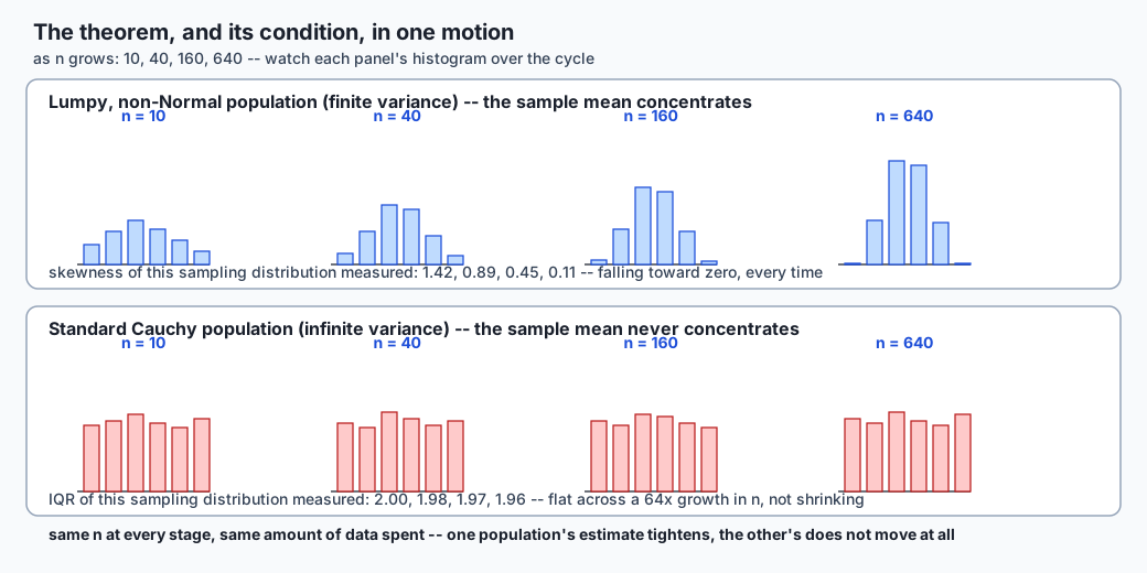
The CLT’s requirement of finite variance is not a technicality. The Cauchy distribution has none — its probability density has tails so heavy that the integral defining its variance (and even its mean) simply does not converge. And the consequence is not “the CLT works more slowly” for Cauchy data. It is that the mean of n Cauchy draws is itself Cauchy distributed, with exactly the same spread, for every single value of n. Averaging a million Cauchy draws is no better than looking at just one.
The lab measures this directly, alongside a well-behaved Exponential population as a control, using the interquartile range (IQR) rather than the standard deviation as the spread measure — deliberately, because a Cauchy sample’s own standard deviation is not an estimate of anything; the quantity it would be estimating does not exist.
| Population | IQR of the sample mean at n=10 | IQR of the sample mean at n=1,000 | Ratio |
|---|---|---|---|
| Exponential (finite variance) | 0.4212 | 0.0428 | 9.85x tighter |
| Standard Cauchy (infinite variance) | 2.0035 | 1.9561 | 1.02x — no change |
A hundred times more data. The Exponential population’s sample mean tightened by almost exactly the sqrt(100) = 10x the CLT predicts. The Cauchy population’s sample mean did not tighten at all — the two IQRs, at n=10 and at n=1,000, differ by 2%, well inside ordinary sampling noise. If you were averaging Cauchy-distributed measurements in production believing “more samples means a tighter estimate,” a thousand-fold increase in your data collection budget would have bought you nothing, and no amount of squinting at the resulting number would tell you that from the number alone — you would need to know the shape of the underlying distribution to know the averaging trick had failed.
Where the CLT fails quietly — dependence
There is a second, subtler way the standard machinery breaks, and it is worse than the Cauchy case precisely because it fails silently. The formula SE = sigma / sqrt(n) assumes the n observations are independent. When they are not — when consecutive observations are correlated, as in a time series, a sequence of requests from the same session, or repeated measurements from the same sensor — the naive formula understates the true standard error.
The lab builds an autocorrelated AR(1) series (each observation is 0.7 times the previous one plus fresh noise) and measures the true standard error the only honest way: generate many independent replications of the whole series and look at the spread of their means. Comparing that to the naive formula applied to a single series:
| Method | Standard error |
|---|---|
| True (from 3,000 independent replications) | 0.1692 |
Naive (sample_std / sqrt(n), single series) | 0.0693 |
The naive formula understates the truth by a factor of 2.44. Nothing about this failure looks wrong from the inside — the naive number is a perfectly ordinary-looking float, computed by a formula that is correct for independent data. The analyst using it becomes confident in exact proportion to how wrong they are, which is precisely why this failure mode is more dangerous in practice than the Cauchy case: a Cauchy distribution announces itself the moment you look at a histogram, but correlated data can look completely unremarkable while quietly making every confidence interval built on it too narrow.
Sampling bias — the failure the mathematics cannot fix
Every result so far describes sampling error: the honest wobble that comes from which particular members of the population happened to land in your sample, and it shrinks as 1/sqrt(n), exactly as promised. Sampling bias is a different failure entirely, and it is the practical lesson worth carrying away from this whole lesson above every other one, because it is the one no amount of additional data rescues you from.
Build a sampler that can only draw from the upper half of a population — values above the population’s own median, no matter how many draws it takes — and compare its behavior to an honest, unrestricted sampler as n grows a hundredfold:
| Sampler | Mean absolute error at n=30 | Mean absolute error at n=3,000 |
|---|---|---|
| Unbiased | 0.4455 | 0.0433 (10.28x smaller) |
| Biased (upper half only) | 2.0712 | 2.0722 (essentially unchanged) |
The unbiased sampler’s error shrinks by almost exactly the sqrt(100) = 10x the standard-error formula predicts. The biased sampler’s error does not move at all — 2.0712 at n=30, 2.0722 at n=3,000, a rounding-level difference. More data made the biased sampler’s confidence interval tighter (because its variance still shrinks, since variance is entirely a property of sampling error) while leaving its accuracy completely unimproved, because its bias is a property of which population it reaches, not of how many draws it takes. This is the single most important practical lesson in this entire day: a confidently precise wrong answer is what sampling bias looks like from the inside, and it looks exactly like a correct answer with a small error bar.
The bootstrap, from scratch
Every standard error above came from a formula (sigma / sqrt(n)) or from brute-force replication of the entire sampling process — a luxury you have in a lab, not in production, where you get exactly one sample and no formula for many statistics of interest. The bootstrap, introduced by Bradley Efron in 1979, solves this with an idea simple enough to implement in a few lines: resample your one dataset with replacement, recompute the statistic on every resample, and read the statistic’s standard error straight off the spread of the results.
Applied to the mean, where a formula exists to check it against: a sample of 200 draws from a population with sigma_hat = 10.07, bootstrapped 5,000 times, gives a bootstrap standard error of 0.7195 against a theoretical sigma_hat / sqrt(200) = 0.7118 — a relative difference of about 1%.
Applied to the median, where no simple closed-form standard error exists at all: the same code, unchanged except for swapping mean for median, gives a bootstrap standard error of 0.5740. Checked for sanity against the only independent yardstick available — the actual spread of medians computed from 2,000 genuinely fresh samples drawn straight from the population — that fresh-sample spread comes out to 0.8824, giving a ratio of 0.65: the same order of magnitude, comfortably within the range of noise expected from estimating a spread of a spread on a single 200-observation dataset. This is the entire reason the bootstrap matters: it gives you a standard error for a statistic no textbook formula covers, using nothing but the data you already have.
An everyday analogy
Carry a single picture through the rest of this lesson: a pollster calling voters before an election.
The population is every eligible voter. The pollster cannot call all of them, so they call a sample — say, 500 people — and ask who they support. The proportion who say “Candidate A” is a statistic, and it is not the true fraction of the whole electorate that supports Candidate A; it is an estimate, built from whichever 500 people happened to pick up the phone. Call a different 500 people tomorrow, get a slightly different number. That variation, purely from who got sampled, is sampling error, and it is what the standard error measures.
The 1/sqrt(n) law is the pollster’s entire budget conversation. Doubling the number of calls does not halve the margin of error — it takes quadrupling the sample, from 500 to 2,000 calls, to cut the margin in half. This is why professional polls converge on sample sizes in the low thousands rather than the low millions: past a certain point, each additional thousand calls buys a shrinking sliver of precision for a linearly growing cost.
The central limit theorem is why the pollster’s confidence interval — “42% support Candidate A, plus or minus 3 points” — is legitimate at all, even though any single respondent’s answer is not remotely bell-shaped; it is a hard 0-or-1. Average enough 0s and 1s together and the distribution of that average, across every possible group of 500 the pollster could have called, is close to Normal-shaped — which is exactly what licenses the “plus or minus 3 points” phrasing and its 95%-confidence meaning.
The Cauchy counterexample has a natural home in this picture too. Imagine a pollster asks not “who do you support” (bounded, 0 or 1) but an unbounded question — “by how many percentage points will your candidate win?” — and a handful of respondents, being facetious or simply extreme, answer things like “plus ten thousand points.” If enough respondents give answers from a distribution with genuinely unbounded, heavy-tailed spread, no amount of additional calling tames the resulting average; one wild answer can dominate the sum regardless of how many sober answers surround it.
And sampling bias is the pollster’s oldest and most notorious failure mode. A poll conducted exclusively by landline telephone, as many were for decades, systematically misses everyone who has only a mobile phone — and if that group votes differently from landline-reachable voters, no number of additional landline calls will ever close the gap. The margin of error can shrink to a fraction of a point while the center of the estimate stays confidently, precisely wrong. This is exactly what happened, at scale, in several real elections where landline-only polling underestimated a demographic shift — the sampling frame, not the sample size, was the problem, and more calls to the same wrong frame only sharpened the wrong answer.
Examples in practice
A model evaluation leaderboard. Two models are evaluated on the same 500-example held-out test set. Model A scores 91.4%; Model B scores 91.1%. The binomial standard error for an accuracy of 91.4% on 500 examples is sqrt(0.914 * 0.086 / 500) ≈ 0.0125, or 1.25 percentage points — and a 0.3-point gap between the two models is only 0.3 / 1.25 ≈ 0.24 standard errors apart. That is well inside the range of pure sampling noise. Reporting Model A as “better” on this evidence alone is exactly the “42 seconds versus 51 seconds” mistake from the opening of this lesson, wearing a different outfit.
A/B testing a checkout flow. Week 17 closes with an A/B Test Analyzer, and every conversion-rate comparison in it rests on this lesson’s machinery: a conversion count out of a fixed number of visitors is a sample proportion, its standard error follows the same binomial formula as the model-evaluation example above, and the honest question is never “which number is bigger” but “how many standard errors apart are they.”
A biased data collection pipeline. A recommendation system’s training data is collected exclusively from users who engage with the current recommendations — the very definition of a system that can only observe the upper half of its own population, in this lesson’s exact structural sense. No amount of additional logged interactions, however voluminous, corrects for the users who never engaged with a bad recommendation in the first place and so never appear in the training data at all. This is precisely exercise 5’s biased-sampler pattern, running in production under the name “selection bias” or “survivorship bias,” and it is why collecting more of the same kind of data is sometimes the least useful thing an ML team can do.
Dependent observations in a monitoring dashboard. A service’s error rate, logged once per minute, is not a sequence of independent draws — an error condition (a downstream outage, a bad deploy) tends to persist across several consecutive minutes. A dashboard that computes a “standard error” on that time series using the naive sample_std / sqrt(n) formula, exactly as this lesson’s exercise 7 does, will report a confidence interval narrower than the truth, in the same direction and for the same reason as the AR(1) measurement above — and the team reading that dashboard will be more confident in a metric in exact proportion to how wrong the confidence interval is.
Implications: security, privacy, performance, scalability, and cost
Cost. The 1/sqrt(n) law is a direct cost curve: if a data-collection or evaluation pipeline costs money per sample — API calls, human annotation, compute for a larger held-out set — then halving your error bar has a fixed 4x cost, and every further halving costs 4x more than the last. Budgeting an evaluation without this law in mind produces one of two failures: over-collecting data for a comparison that a much smaller sample would have already resolved, or under-collecting data and reporting a difference that is really just noise.
Scalability. Sampling exists specifically because full-population measurement does not scale, and the standard error is the tool that tells you how much sample you actually need before you have “enough.” A system that estimates a metric from a random 1% sample of production traffic, rather than logging and processing everything, is trading exactness for a known, quantifiable amount of noise — and the CLT is what makes that trade honest rather than reckless.
Performance and reproducibility. Every simulation and Monte Carlo estimate in this course (and in production ML — dropout-based uncertainty estimates, ensemble disagreement, sampling-based evaluation) inherits this lesson’s machinery directly. A pipeline that reports a metric without a standard error is not more precise than one that does; it is simply not telling you how much to trust the number, and two runs of the same pipeline with different random seeds can legitimately disagree by an amount this lesson teaches you to compute in advance.
Privacy. Sampling is also a privacy tool: many differential-privacy mechanisms rely on adding calibrated noise to a query result, and the amount of noise needed to protect an individual while preserving a useful signal is directly informed by how the underlying statistic’s own sampling variability behaves. A metric with a naturally large standard error can absorb more added privacy noise for the same practical utility than one with a tight, well-behaved sampling distribution.
Security. The dependence failure mode has a security-adjacent cousin: an attacker who can influence which observations enter a monitored sample (for instance, timing malicious requests to correlate with legitimate traffic, or flooding a system during a specific window) is effectively inducing exactly the kind of autocorrelation exercise 7 measures, quietly widening the true uncertainty of any metric computed naively from that traffic and making an anomaly-detection threshold based on the naive standard error easier to slip beneath.
Alternatives: free, open source, and commercial
numpy.random.Generator — free, BSD 3-Clause licence. When to choose it: any time you need fast, vectorised, seeded random sampling in Python — every exercise in this lesson’s lab runs through it. How: construct one explicit Generator per independent stream of randomness with rng = numpy.random.default_rng(seed), and pass that object into every function that needs it, rather than reseeding inside each function — several of this lesson’s own tolerances would silently fail if a function built a fresh, unseeded generator internally instead of accepting rng as a parameter. Concrete example: rng.integers(0, population.shape[0], size=(trials, n)) builds the index array for trials independent samples of size n in one vectorised call, which is exactly how this lesson’s sampling_distribution function draws tens of thousands of samples without a Python-level loop. Free vs paid: entirely free, and what was actually run for every measurement in this lesson.
The statistics module (Python standard library) — free, part of every Python 3 install. When to choose it: a quick, dependency-free mean, standard deviation, or variance on a plain list, without pulling in NumPy at all. How: statistics.mean(data), statistics.stdev(data) (sample standard deviation, n-1 divisor). Concrete example: statistics.stdev([1.0, 2.0, 3.0, 4.0, 5.0]) gives the same sample standard deviation as numpy.std(data, ddof=1). Free vs paid: entirely free; this lesson ran it directly on the fixed sample used in the bootstrap exercise as a cross-check against NumPy’s own .std(ddof=1), and the two agreed to full float precision.
scipy.stats — free, BSD 3-Clause licence, but not installed in this authoring environment, so no output from it is reproduced anywhere in this lesson or its lab. scipy.stats.sem computes a sample’s standard error of the mean directly, in one call, doing what exercise 1’s theoretical_standard_error does by formula. scipy.stats.bootstrap implements the resample-and-recompute technique of exercise 6 with several confidence-interval methods (percentile, basic, and bias-corrected-and-accelerated) built in, batched for speed. When you would choose it: any production use of the bootstrap, where the engineering behind an accelerated confidence interval is worth not re-deriving. How it would be called: scipy.stats.bootstrap((data,), numpy.median, n_resamples=5000, method='percentile') returns a confidence interval object with a .standard_error attribute — the same number exercise 6 computes by hand. This lesson describes both functions from their public documentation and states plainly that neither was run here.
pandas’ DataFrame.sample — free, BSD 3-Clause licence, not installed here; described from documentation only. When to choose it: sampling rows from a tabular dataset already loaded into a DataFrame, with options for sampling with or without replacement and for weighted sampling. How it would be called: df.sample(n=40, replace=True, random_state=rng) draws a sample of 40 rows with replacement, accepting the same numpy.random.Generator object this lesson uses everywhere else, which is the detail that matters most for reproducibility in a larger pipeline that mixes NumPy and pandas sampling. No output from pandas is reproduced anywhere in this lesson.
Excel / Google Sheets — free (Sheets) or bundled with a paid office subscription (Excel). When to choose them: a one-off standard-error calculation for a non-technical audience, or a quick sanity check beside a spreadsheet a colleague already maintains. How: =STDEV.S(range)/SQRT(COUNT(range)) computes the standard error of the mean directly in a cell. Concrete example: for the bootstrap exercise’s 200-value sample, this formula would return the same 0.7118 this lesson computed as sigma_hat / sqrt(200). Free vs paid: Google Sheets is free; Excel’s current pricing is not reproduced here because it changes independently of this lesson.
Comparison with related concepts
| Concept | What it measures or claims | Shrinks with more data? |
|---|---|---|
| Standard deviation (population or sample) | The spread of individual observations | No — it estimates a fixed property of the population |
| Standard error | The spread of a statistic (like the sample mean) across repeated samples | Yes, as 1/sqrt(n), given finite variance and independence |
| Law of large numbers | The sample mean converges to the true mean | Not a rate claim — only says convergence happens |
| Central limit theorem | The sampling distribution’s shape (Normal) and rate (1/sqrt(n)) | Is itself the claim about how fast |
| Sampling bias | A mismatch between the sampling frame and the target population | No — never shrinks with more of the same kind of data |
| Bootstrap standard error | An estimate of a statistic’s standard error, from resampling one dataset | Its own precision improves with more bootstrap resamples, but it estimates a quantity that itself shrinks as 1/sqrt(n) in the original sample size |
The standard deviation and the standard error are the pair most often confused, and the confusion is understandable because they share a formula’s DNA — the standard error of the mean literally is sigma / sqrt(n), built from the standard deviation. But they answer different questions: “how spread out is any one measurement” versus “how spread out is the average of n measurements.” A clinical trial reporting patient blood pressures might reasonably show a standard deviation of 15 mmHg (individuals vary a lot) alongside a standard error of the mean blood pressure of 1.5 mmHg (with a large enough sample, the average is pinned down far more tightly than any individual reading) — both numbers are correct, and reporting one where the other is needed is a common and consequential mistake.
When to use it — and when not to
Use a standard-error-based confidence statement when: you are reporting any statistic computed from a sample and someone downstream will make a decision based on it — a model comparison, an A/B test result, a survey finding, a monitoring metric. If you cannot state how much a number could plausibly have differed under a different sample, you have reported a number, not a finding.
Reach for the bootstrap specifically when: the statistic you care about has no simple closed-form standard error — the median, a ratio of two sums, a correlation coefficient, a custom business metric — and you have one dataset rather than the ability to repeat the whole experiment.
Do not trust the naive sigma / sqrt(n) formula when: your observations are not independent — a time series, repeated measurements from the same unit, clustered survey responses (multiple people from the same household, multiple requests from the same session). Exercise 7’s AR(1) result generalizes: any positively autocorrelated data will make the naive formula understate the truth, sometimes severely.
Do not expect the CLT to rescue you when: the underlying population plausibly has infinite variance — genuinely heavy-tailed phenomena like some network latency distributions under contention, viral content view counts, or certain financial returns. In those cases, check the spread with something robust to tail weight (the IQR, or a trimmed mean) before trusting any standard-deviation-based error bar, and consider whether the mean is even the statistic you should be reporting.
Never treat a shrinking confidence interval as evidence against bias. A tight interval tells you sampling error is small. It says nothing about whether your sampling frame reaches the population you actually care about. That question has to be answered by examining how the data was collected, not by collecting more of it.
Knowledge check
- A team measures average session length as 42 seconds from one sample of 30 users, then 51 seconds from a fresh sample of 30 users from the same population the following week. What does this demonstrate?
- Why does the standard error shrink as
1/sqrt(n)rather than1/n— what does quadruplingndo to the standard error, and what would need to be true for it to halve instead? - State the difference between the law of large numbers and the central limit theorem in one sentence each.
- Why does averaging more Cauchy-distributed draws fail to tighten the estimate of their “mean,” when averaging more Exponential-distributed draws does tighten the estimate?
- A biased sampler’s confidence interval gets tighter as
ngrows, even though its estimate stays far from the truth. Explain why both of those things are true at once. - What does the bootstrap actually do, in one sentence, and why is it applied to the median in this lesson rather than only to the mean?
- Why does autocorrelation in a dataset make the naive standard-error formula understate the truth, rather than overstate it or leave it unaffected?
- A model scores 91.4% on a 500-example test set and a competing model scores 91.1% on the same set. Using the binomial standard error, is this difference meaningful? Show the calculation.
Hands-on exercise
Build and run the lab, “Sampling You Can Trust,” in labs/sections/math-statistics-and-data/day-117-sampling-and-the-central-limit-theorem/. Nine exercises, each checked two ways — a formula where one exists, a seeded simulation with a tolerance derived from a standard error or a ratio band otherwise, never a guessed number.
cd labs/sections/math-statistics-and-data/day-117-sampling-and-the-central-limit-theorem
python3 -m venv .venv
.venv/bin/pip install -r requirements/requirements.txt
Work through starter/00_brief.md, filling in starter/sampling.py one function at a time, checking yourself as you go with .venv/bin/pytest starter -q. Unattempted exercises report as skipped; wrong ones fail with your value printed beside the correct one.
Expected output
Once every exercise is written, the full harness:
bash tests/run_tests.sh
echo "exit=$?"
ends with:
32 checks, 0 failure(s).
exit=0
The single result most worth internalizing before you meet it, from exercise 4:
Exponential(scale=1.0): IQR of the mean at n=10 = 0.4212, at n=1000 = 0.0428
  ratio = 9.85  (100x more data, expected shrink ~ sqrt(100) = 10x)

standard Cauchy: IQR of the mean at n=10 = 2.0035, at n=1000 = 1.9561
  ratio = 1.02  (100x more data, expected shrink: NONE)
Validate your work
Run .venv/bin/pytest examples -q -p no:cacheprovider and confirm 19 passed. Run each of the nine reference scripts in examples/ directly and confirm each prints every assertion held. on its last line. Confirm .venv/bin/pytest starter -q -p no:cacheprovider reports 13 passed once every exercise is filled in, with no failure you were not expecting.
Troubleshooting
See troubleshooting.md in the lab directory for the full list, including the wrong-directory import error, the tolerance failures that trace back to a function building its own unseeded rng instead of accepting one as a parameter, and the __pycache__ search that must prune .venv.
Common mistakes
Using the standard deviation instead of the IQR when comparing the Cauchy population’s spread (exercise 4) — it produces a number that looks like an ordinary float and estimates nothing. Filtering the biased sampler against the wrong array or with the wrong comparison operator in exercise 5, which silently produces a “biased” sampler that behaves almost like the unbiased one. Getting the AR(1) innovation variance wrong in exercise 7 (it must be sigma * sqrt(1 - phi**2), not sigma), which changes what the exercise is actually measuring.
Practice assignment
Pick a metric you have access to — a personal fitness tracker’s daily step count, a household’s monthly electricity usage, or (if you have programming access to one) a small public dataset. Draw at least 30 independent samples of size n for two different values of n that differ by a factor of 4, compute the sample mean each time, and measure the standard deviation of those means — your own empirical standard error. Compare it to the population’s own standard deviation divided by sqrt(n), and write down, in your own words, what the ratio between your two standard errors tells you about the 1/sqrt(n) law using your own data rather than this lesson’s.
Extension challenge
Extend exercise 4 to the Student’s t-distribution, which is the Cauchy distribution’s less pathological cousin: the Cauchy distribution is exactly the t-distribution with 1 degree of freedom. Using numpy.random.Generator.standard_t(df), repeat the IQR-shrinkage measurement at df equal to 1, 2, 5 and 30, and find the smallest degrees-of-freedom value at which the sample mean’s IQR shrinks by at least 5x going from n=10 to n=1,000. At what point does a heavy-tailed distribution become “heavy enough” to defeat the central limit theorem in a way that matters for a sample size you can realistically collect?
Quiz
Q1. Two samples of 30 users, drawn from the exact same population, give average session lengths of 42 seconds and 51 seconds. What does this demonstrate?
- One of the two measurements must contain an error
- The population itself changed between the two measurements
- A sample statistic is itself a random variable with its own distribution, so two honest samples can legitimately disagree
- Session length is not a valid metric to measure this way
Show answer
Answer: C. A sample statistic is itself a random variable with its own distribution, so two honest samples can legitimately disagree
Nothing was done incorrectly in either measurement. A sample mean is a function of which particular users happened to land in the sample, and different samples produce different means -- that variation is exactly what a sampling distribution and its standard error describe. Reporting either 42 or 51 as "the" answer, without the spread, is the mistake this lesson exists to prevent.
Q2. The standard error of the mean is sigma / sqrt(n). If n is quadrupled from 100 to 400, what happens to the standard error?
- It falls to one half of its previous value
- It falls to one quarter of its previous value
- It stays the same, since only the variance changes with n
- It falls to one sixteenth of its previous value
Show answer
Answer: A. It falls to one half of its previous value
sqrt(400)/sqrt(100) = 20/10 = 2, so the standard error is divided by 2, not 4. This lesson measured it directly across four sample sizes each 4x the last (10, 40, 160, 640) and found ratios of 1.985, 1.991 and 2.011 -- consistently near 2.0, and the compounded ratio from n=10 to n=640 came out to 7.95 against a predicted sqrt(64)=8.00, nowhere near the 64x a 1/n law would predict.
Q3. What is the difference between the law of large numbers and the central limit theorem?
- They are two names for the same result
- The LLN applies only to discrete random variables and the CLT only to continuous ones
- The CLT is a special case of the LLN that only applies to Normal populations
- The LLN says the sample mean converges to the true mean; the CLT says how fast (1/sqrt(n)) and what shape the errors take (Normal, given finite variance)
Show answer
Answer: D. The LLN says the sample mean converges to the true mean; the CLT says how fast (1/sqrt(n)) and what shape the errors take (Normal, given finite variance)
This is the distinction most commonly conflated. Jacob Bernoulli's 1713 result (published posthumously in Ars Conjectandi) established convergence -- more data gets you closer to the truth. It says nothing about the rate or the shape of the errors along the way. The central limit theorem, building on Abraham de Moivre's 1733 result and generalized by Pierre-Simon Laplace, supplies exactly that missing rate and shape.
Q4. An Exponential population's sample mean tightens by about 9.85x from n=10 to n=1,000 (a 100x increase in data). A standard Cauchy population's sample mean, measured the same way, shows a ratio of only 1.02x. What explains the difference?
- The Cauchy measurement used too few trials to detect the shrinkage
- The Exponential population happened to have unusually low variance in this run
- The Cauchy distribution has no defined mean or variance, so the mean of n Cauchy draws is itself Cauchy distributed with the same spread for every n -- the central limit theorem's finite-variance condition fails outright
- The IQR is not a valid spread measure for comparing the two distributions
Show answer
Answer: C. The Cauchy distribution has no defined mean or variance, so the mean of n Cauchy draws is itself Cauchy distributed with the same spread for every n -- the central limit theorem's finite-variance condition fails outright
This is the central limit theorem's condition, not decoration. Averaging more Cauchy draws is mathematically no better than looking at a single one, because there is no finite population variance for the averaging process to shrink toward. The interquartile range (IQR) is used specifically because a Cauchy sample's own standard deviation is not an estimate of anything -- the quantity it would estimate does not exist.
Q5. A sampler restricted to drawing only from the upper half of a population shows a mean absolute error of 2.0712 at n=30 and 2.0722 at n=3,000 -- essentially unchanged despite 100x more data. An honest sampler's error shrinks from 0.4455 to 0.0433 (10.28x) over the same range. What does the biased sampler's result demonstrate?
- The biased sampler needs an even larger n before its error will start shrinking
- The mean absolute error formula was applied incorrectly
- Both samplers actually behaved the same way, within rounding
- Sampling bias does not shrink with more data, because it is a mismatch between the sampling frame and the target population, not sampling error -- more data buys a more precise estimate of the wrong number
Show answer
Answer: D. Sampling bias does not shrink with more data, because it is a mismatch between the sampling frame and the target population, not sampling error -- more data buys a more precise estimate of the wrong number
This is the practical lesson the mathematics cannot rescue you from. The biased sampler's confidence interval DOES get tighter as n grows, because its variance still shrinks -- but its center stays fixed on the biased pool's mean, which is not the true population mean. A confidently precise wrong answer is exactly what sampling bias looks like from the inside, and no amount of additional data collected the same way fixes it.
Q6. The bootstrap standard error of a sample mean (0.7195) is checked against the formula sigma_hat/sqrt(n) (0.7118) and agrees within about 1%. The same bootstrap code is then applied to the sample median, giving 0.5740. Why is this second result checked against fresh samples rather than a formula?
- Because the median is always less reliable than the mean and should never be trusted
- Because no simple closed-form standard error exists for the median, which is precisely why the bootstrap -- resample, recompute, read off the spread -- is a genuinely useful technique rather than a redundant one
- Because bootstrapping only works correctly for the arithmetic mean
- Because the median formula is too complicated to implement in this lab
Show answer
Answer: B. Because no simple closed-form standard error exists for the median, which is precisely why the bootstrap -- resample, recompute, read off the spread -- is a genuinely useful technique rather than a redundant one
The mean case is a sanity check on the method, using a statistic where an independent formula exists to compare against. The median case is the actual point of the exercise: the exact same resample-and-recompute code, unchanged, produces a usable standard error for a statistic that has no simple formula at all -- checked here against the spread of medians from genuinely fresh, independent samples of the same population.
Q7. An autocorrelated (AR(1)) series has a true standard error, measured by replication, of 0.1692. The naive sample_std/sqrt(n) formula applied to a single series gives 0.0693 -- less than a third of the truth. Why is this a more dangerous failure than the Cauchy counterexample?
- It is not more dangerous; both are equally obvious once you compute a number
- Autocorrelation always makes the naive standard error too LARGE, which is a safer direction to be wrong in
- This failure only occurs with financial time-series data and is not relevant elsewhere
- The naive formula looks completely ordinary -- a plausible float from a correct-for-independent-data formula -- so nothing about the output signals that anything has gone wrong, unlike a Cauchy histogram, which announces its heavy tails visually
Show answer
Answer: D. The naive formula looks completely ordinary -- a plausible float from a correct-for-independent-data formula -- so nothing about the output signals that anything has gone wrong, unlike a Cauchy histogram, which announces its heavy tails visually
The naive standard error understates the truth here by a factor of 2.44, and it does so silently: the formula is arithmetically correct, the output is a normal-looking float, and nothing about the number itself signals a problem. An analyst trusting it becomes confident in exact proportion to how wrong they are -- this is why the lesson calls dependence a QUIET failure, in contrast to the Cauchy case, which a histogram exposes immediately.
Q8. A model scores 91.4% on a 500-example held-out test set, and a rival model scores 91.1% on the same set -- a 0.3 percentage-point gap. Using the binomial standard error formula, what does this gap represent?
- A gap that cannot be evaluated without knowing the exact examples in the test set
- A statistically significant improvement, since the raw percentage went up
- A 0.3-point gap that is always meaningful regardless of test-set size
- The binomial standard error is about 1.25 percentage points, so the 0.3-point gap is only about 0.24 standard errors -- well inside the range of pure sampling noise, demonstrating essentially nothing
Show answer
Answer: D. The binomial standard error is about 1.25 percentage points, so the 0.3-point gap is only about 0.24 standard errors -- well inside the range of pure sampling noise, demonstrating essentially nothing
sqrt(0.914 * 0.086 / 500) is approximately 0.0125, or 1.25 percentage points. A 0.3-point difference is a small fraction of one standard error. Leaderboard comparisons smaller than the standard error are noise, not evidence -- which is exactly why held-out evaluation sets need to be large: shrinking the standard error to make small real differences detectable requires the same 1/sqrt(n) law measured throughout this lesson.
Glossary
- Population
- The complete set of things you would measure if you could measure everything -- every user, every possible model output, every unit that could ever be produced. Almost always too large, too expensive, or too undefined (still growing, still being generated) to measure directly, which is the entire reason sampling exists.
- Sample
- The subset of the population actually observed. A sample of size n drawn "with replacement" allows the same population member to appear more than once; this lesson's lab draws every sample this way, which is what lets a finite array stand in for an effectively infinite population.
- Estimator
- A rule for turning a sample into a number that estimates some property of the population -- the sample mean estimating the population mean, the sample proportion estimating the true rate. An estimator is itself a function of the random sample, which is exactly why it is a random variable with its own distribution.
- Sampling distribution
- The distribution of a statistic's value across every sample the sampling process could have produced. Not a single number and not the population -- a genuinely separate object, built in this lesson's lab by literally repeating the draw-a-sample-and-compute-the-mean process thousands of times and studying the resulting array of means.
- Standard error
- The standard deviation of a statistic's own sampling distribution -- how much the statistic itself wobbles from sample to sample. For the sample mean, the standard error equals sigma / sqrt(n), where sigma is the population's standard deviation. Not the same quantity as the population's own standard deviation, which describes individual observations rather than the average of several of them.
- The sqrt(n) law
- The consequence of the standard error formula that quadrupling the sample size roughly halves the standard error, not quarters it. Measured directly across four sample sizes each 4x the last (10, 40, 160, 640), the ratios came out to 1.985, 1.991 and 2.011, against a predicted 2.0 at every step.
- Central limit theorem (CLT)
- The result that, whatever shape a population has, the sampling distribution of its mean approaches a Normal distribution as n grows, provided the observations are independent and the population has finite variance. First appeared as a special case in Abraham de Moivre's 1733 work on the Binomial distribution, generalized by Pierre-Simon Laplace by 1812, and given its modern name by George Polya in 1920.
- Law of large numbers (LLN)
- Jacob Bernoulli's 1713 result that a sample mean converges to the true population mean as the sample size grows. A weaker claim than the central limit theorem: the LLN says convergence happens; the CLT says how fast (1/sqrt(n)) and what shape the errors take (Normal, given finite variance) along the way.
- Cauchy distribution
- A continuous distribution, named for Augustin-Louis Cauchy, with no defined mean or variance -- its tails are too heavy for either integral to converge. The standard counterexample to the central limit theorem: the mean of n Cauchy draws is itself Cauchy distributed, with exactly the same spread, for every value of n. Measured in this lesson's lab, its sample mean's interquartile range changed by only 2% from n=10 to n=1,000, against an Exponential population's 9.85x tightening over the same range.
- Interquartile range (IQR)
- The 75th percentile minus the 25th percentile of a sample -- a spread measure that depends only on the order of the data, not on its moments. Used in place of the standard deviation when comparing the Cauchy and Exponential sampling distributions, because a Cauchy sample's own standard deviation is not an estimate of anything: the population variance it would estimate does not exist.
- Sampling error
- The honest wobble in a statistic that comes purely from which particular population members happened to land in the sample. Shrinks as 1/sqrt(n), exactly as the standard error formula predicts, and is what every standard error and confidence interval in this lesson measures.
- Sampling bias
- A systematic mismatch between the population a sampling frame actually reaches and the population being claimed. Unlike sampling error, it does not shrink with n at all: measured in this lesson's lab, a sampler restricted to the upper half of a population showed a mean absolute error that stayed essentially flat (2.0712 versus 2.0722) across a hundredfold growth in sample size, while an honest sampler's error shrank by 10.28x over the same range.
- Bootstrap
- A technique, introduced by Bradley Efron in 1979, for estimating a statistic's standard error by resampling one dataset with replacement, recomputing the statistic on each resample, and reading the standard error off the spread of the results -- no formula for the statistic's own sampling distribution required. Checked in this lesson against a known formula for the mean (agreement within about 1%) and applied to the median, where no formula exists.
- AR(1) process
- An autoregressive series of order 1: each observation equals phi times the previous observation plus fresh, independent noise. Used in this lesson to build a dataset with genuine dependence between consecutive observations, on which the naive standard-error formula is measured to understate the truth by more than a factor of two.
- Binomial standard error
- The standard error of a sample proportion (equivalently, a model accuracy measured on n examples): sqrt(phat * (1 - phat) / n). For an accuracy of 91.4% on 500 examples, this comes out to about 1.25 percentage points -- large enough that a 0.3-point difference between two models sits at only about 0.24 standard errors, well inside the range of pure sampling noise.
Sources and further reading
- Random Generator — NumPy documentation — NumPy Developers (accessed 2026-08-17)
- numpy.random.Generator.standard_cauchy — NumPy documentation — NumPy Developers (accessed 2026-08-17)
- statistics — Mathematical statistics functions — Python Software Foundation (accessed 2026-08-17)
- scipy.stats — SciPy documentation — SciPy Developers (accessed 2026-08-17)
- Introduction to Probability — Dartmouth College (accessed 2026-08-17)
Kept in this browser, no account needed. Your progress page turns the whole record into one link you can bookmark or open on another device.