Machine Learning › Unsupervised Learning › Day 186
Day 186: t-SNE and UMAP
Master non-linear manifold learning: formulate t-SNE with perplexity and Student-t distributions to solve the crowding problem, and leverage UMAP for Riemannian manifold preservation and fast parametric projection.
Hands-on lab for this lesson
Lab files on GitHub: https://github.com/ai-roadmap-365/ai-roadmap-365.github.io/tree/main/labs/sections/machine-learning/day-186-t-sne-and-umap
- Get the hands-on files. Clone the labs repository once (you can reuse this clone for every lesson). This works on macOS, Linux, and Windows (PowerShell or WSL):
git clone https://github.com/ai-roadmap-365/ai-roadmap-365.github.io.git cd ai-roadmap-365.github.io - Open this lesson's lab. Move into the directory for this specific day. Every lab lives at the same predictable path — section / subsection / week / day:
cd labs/sections/machine-learning/day-186-t-sne-and-umap - Read the lab guide. Open `README.md` in that directory. It lists the exact commands, what each does, the expected output, and how to check your work — read it before running anything.
- Run it and check your work. Follow the README's "How to run" section: run the example first to see the finished result, then complete the numbered exercises in `starter/`, then run the tests. The tests pass (exit 0) only when your work is correct.
bash tests/run_tests.sh # or the test command named in the lab README
You can also open the lab as a local page (works offline, shows the file tree and expected output).
Learning objectives
By the end of this lesson you will be able to:
- Formulate the high-dimensional Gaussian affinities and low-dimensional Student-t joint probabilities in t-SNE.
- Derive the Kullback-Leibler (KL) divergence gradient optimization for t-SNE.
- Explain the Crowding Problem and how Cauchy heavy tails alleviate embedding congestion.
- Formulate UMAP Riemannian manifold assumptions, fuzzy simplicial sets, and cross-entropy loss.
- Tune Perplexity, Early Exaggeration, n_neighbors, and min_dist for exploratory data analysis.
Prerequisites
- [object Object]
Yesterday, we mastered Principal Component Analysis (PCA). PCA is mathematically optimal, closed-form, and blazing fast. However, PCA is strictly a linear projection technique.
When data lies on a complex curved manifold — such as the celebrated Swiss Roll, intertwined double helices, single-cell RNA transcriptomes, or deep neural network latent activation spaces — linear projections flatten and crush distinct topological structures onto one another, causing completely unrelated classes to overlap.
To visualize and explore complex non-linear geometry, we turn to Non-Linear Manifold Learning. The two modern titans of non-linear visualization and representation are:
- t-SNE (t-Distributed Stochastic Neighbor Embedding): Introduced by Laurens van der Maaten and Geoffrey Hinton in 2008.
- UMAP (Uniform Manifold Approximation and Projection): Introduced by Leland McInnes, John Healy, and James Melville in 2018.
Today, we dive deep into the probability formulations, crowding problem resolution, gradient mechanics, and practical tuning of t-SNE and UMAP.
Why this matters
Non-linear manifold visualization is essential across cutting-edge science and production AI:
- Single-Cell Genomics (scRNA-Seq): Biologists sequence 100,000 individual cells measuring 20,000 gene expressions. UMAP reveals continuous cellular differentiation trajectories, branching from stem cells into specialized lineages.
- Deep Learning Latent Space Auditing: Computer vision and LLM engineers inspect penultimate embedding spaces (e.g. CLIP or BERT embeddings) using t-SNE to diagnose class confusion, representation collapse, and out-of-distribution drift.
- High-Frequency Financial Anomaly Inspection: Quant researchers project 200 market microstructure features into 2D manifolds to visually identify market regimes and flash-crash precursors.
- Speech and Audio Representation: Visualizing acoustic phoneme clusters produced by audio self-supervised models (Wav2Vec2, Whisper).
The idea in plain language
Imagine a world atlas:
- The planet Earth is a curved 3D spherical surface.
- If you simply squish the globe flat with a hydraulic press (a linear projection), North America and Asia crush together, distances distort horribly, and Antarctica wraps into a distorted ring.
- Manifold Learning is like carefully peeling the skin of an orange: you make small incisions in empty oceans so that every continent retains its true local shape, distances, and neighborhood cities when laid flat on a 2D tabletop.
The Key Difference: t-SNE vs UMAP
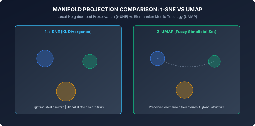
- t-SNE cares almost exclusively about local neighbors: “Keep my 30 closest friends together on the table; I don’t care where the other continents land.”
- UMAP balances local neighborhoods with global continental layout: “Keep my closest friends together, but also ensure Europe is positioned relative to Asia and Africa in an orderly global structure.”
Historical background
- 2002 (Geoffrey Hinton and Sam Roweis): Introduced Stochastic Neighbor Embedding (SNE), converting Euclidean distances into conditional Gaussian probabilities. SNE suffered from severe optimization difficulties and the crowding problem.
- 2008 (Laurens van der Maaten and Geoffrey Hinton): Published Visualizing Data using t-SNE in JMLR. They introduced two key innovations: symmetrized joint probabilities and replacing the low-dimensional Gaussian with a heavy-tailed Student-t (Cauchy) distribution.
- 2014 (Laurens van der Maaten): Developed Barnes-Hut t-SNE, using spatial quad-trees to reduce computational complexity from O(N^2) to O(N log N).
- 2018 (Leland McInnes et al.): Published UMAP, framing manifold learning using Riemannian geometry and fuzzy simplicial sets. UMAP achieved massive speedups and superior preservation of global data structure.
What it is — and what it is not
What t-SNE and UMAP ARE:
- Non-Parametric Manifold Visualizers: They find low-dimensional coordinates Y in R^(N x 2) that preserve high-dimensional pairwise probabilistic relationships.
- Exploratory Tools: Designed to discover cluster separations, sub-populations, and continuous manifolds.
- Non-Linear Dimensionality Reducers: Capable of unrolling complex curved surfaces (e.g. Swiss Roll, spheres, tori).
What they are NOT:
- Not Distance-Preserving Metric Projections: Distances between distant clusters in a t-SNE plot have zero metric meaning; cluster sizes and inter-cluster gaps in t-SNE are heavily influenced by perplexity and density.
- Not Out-of-Sample Transformers (by default): Unlike PCA where
pca.transform(X_new)projects new points instantly, standard t-SNE cannot project new samples without re-running optimization (though UMAP supports parametric mapping). - Not Clustering Algorithms: t-SNE and UMAP produce 2D coordinate projections; downstream clustering algorithms (like HDBSCAN or K-Means) must be run on the coordinates to assign labels.
Why it was created and what problems it solves
Linear methods (PCA, Classical Multidimensional Scaling) preserve large pairwise distances at the expense of small local neighborhoods. In high dimensions, the vast majority of points are far apart, causing linear algorithms to focus on distant pairs while smearing fine local clusters into an undifferentiated blob.
Furthermore, classical non-linear techniques like Isomap (geodesic shortest paths) and Locally Linear Embedding (LLE) suffer from topological short-circuiting: a single noise point in the void between two manifold folds creates an artificial shortcut that corrupts the entire global distance matrix.
t-SNE and UMAP solved these historical challenges by replacing rigid global distance metrics with smooth, probabilistic neighborhood matching that naturally down-weights distant outliers while emphasizing tight local structure.
How it works
Let us dissect the mathematical formulation of both t-SNE and UMAP in comprehensive detail.
1. High-Dimensional Probability Affinities in t-SNE
Given N samples in R^D, t-SNE measures the probability p_(j|i) that point x_i picks point x_j as its neighbor under a Gaussian distribution centered at x_i:
p_{j|i} = exp(-||x_i - x_j||^2 / (2 * sigma_i^2)) / sum_{k != i} exp(-||x_i - x_k||^2 / (2 * sigma_i^2))with p_(i|i) = 0.
Setting sigma_i via Perplexity:
The variance sigma_i^2 is determined individually for each point such that the Shannon entropy of the conditional distribution matches a user-specified Perplexity:
Perplexity(P_i) = 2^{H(P_i)} = 2^{-sum_j p_{j|i} log_2 p_{j|i}}Typical perplexity values range between 5 and 50 (representing the effective number of nearest neighbors). In dense regions, sigma_i is small; in sparse regions, sigma_i automatically expands.
Symmetrized Joint Probabilities:
To handle outliers robustly, t-SNE defines the symmetric joint probability p_ij:
p_ij = (p_{j|i} + p_{i|j}) / (2 * N)This guarantees that every observation contributes at least (1 / (2*N)) to the total probability mass, preventing isolated outlier points from having zero gradient influence.
2. Low-Dimensional Affinities and the Crowding Problem
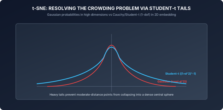
In the low-dimensional embedding space Y in R^(N x 2), t-SNE models affinities using a Student-t distribution with 1 degree of freedom (standard Cauchy distribution):
q_ij = (1 + ||y_i - y_j||^2)^{-1} / sum_{k} sum_{l != k} (1 + ||y_k - y_l||^2)^{-1}Why the Student-t Distribution Solves Crowding:
In D-dimensional space, the volume of a sphere of radius r scales as r^D. There is vast volume available for moderate-distance points. When projected into 2D, the available area scales only as r^2.
If we used a Gaussian distribution in 2D, moderate-distance points would be forced to crowd tightly together around the origin. Because the Student-t distribution has heavy polynomial tails ((1 + d^2)^-1 vs exp(-d^2)), moderate-distance points in the map can spread far apart while maintaining small probability values matching high-dimensional affinities.
3. The Objective: Kullback-Leibler (KL) Divergence
t-SNE minimizes the KL divergence between high-dimensional distribution P and low-dimensional distribution Q:
L_KL = KL(P || Q) = sum_{i=1}^N sum_{j=1}^N p_ij * log(p_ij / q_ij)The analytic gradient with respect to low-dimensional coordinate y_i is:
nabla_{y_i} L = 4 * sum_{j=1}^N (p_ij - q_ij) * (y_i - y_j) * (1 + ||y_i - y_j||^2)^{-1}This gradient behaves like a system of physical springs:
- Attractive Forces: Points with high p_ij pull each other together with force proportional to p_ij * (1 + ||y_i - y_j||^2)^-1.
- Repulsive Forces: The q_ij term pushes all points apart, preventing collapse.
Optimization Mechanics: Early Exaggeration and Momentum
Gradient descent in t-SNE relies on two critical heuristics:
- Early Exaggeration: During the first 100 to 250 iterations, all p_ij values are multiplied by a constant factor (typically 4.0 or 12.0). This creates enormous attractive forces that pull natural clusters into tight, dense balls. Because the space between clusters is large and relatively empty, clusters can easily navigate around one another to find their optimal global layout without getting tangled.
- Adaptive Learning Rates and Momentum: Standard momentum starts at 0.5 and switches to 0.8 after early exaggeration ends, preventing oscillation.
4. UMAP: Riemannian Geometry and Fuzzy Simplicial Sets
UMAP is founded on rigorous mathematical concepts from algebraic topology and Riemannian geometry:
- Riemannian Metric Assumption: Data is assumed to lie on a smooth Riemannian manifold where the metric tensor is locally constant.
- Local Metric Scaling: Distance is scaled locally around each point by rho_i (the distance to its nearest neighbor) and sigma_i (a normalizing factor ensuring sum_(j) exp(-max(0, d(x_i, x_j) - rho_i) / sigma_i) = log2(k)).
- Fuzzy Simplicial Set Assembly: Local metric spaces are combined into a global fuzzy topological representation using fuzzy set union (algebraic t-conorm): mu_(i union j) = mu_i + mu_j - mu_i * mu_j.
UMAP Loss: Fuzzy Set Cross-Entropy
Instead of KL divergence, UMAP optimizes the Binary Fuzzy Cross-Entropy:
L_UMAP = sum_{e in E} [ p_e * log(p_e / q_e) + (1 - p_e) * log((1 - p_e) / (1 - q_e)) ]- The first term
p_e * log(p_e / q_e)provides Attractive Forces (pulling nearest neighbors together). - The second term
(1 - p_e) * log((1 - p_e) / (1 - q_e))provides Repulsive Forces (pushing non-neighbors apart).
Because the repulsive term acts globally on all non-edges via stochastic negative sampling, UMAP preserves broad global trajectories, continuous branchings, and relative distances with far greater fidelity than t-SNE.
Practical Hyperparameters in UMAP:
n_neighbors: Balances local vs global structure (typical values: 15 to 50). Small values focus on fine-grained local manifolds; large values capture macro-scale global topology.min_dist: Controls how tightly points are packed in 2D (typical values: 0.1 to 0.5). Lower values produce dense clumpy clusters; higher values create diffuse, spread-out clouds.
An everyday analogy
Think of arranging 100 students at a school dance:
- PCA: The photographer stands on a balcony and takes a top-down aerial photo. Students standing in straight lines are clear, but anyone standing in circles or beneath the balcony gets squished.
- t-SNE: You attach rubber bands between students who are best friends. You release them onto the gym floor and let the rubber bands snap them into tight social cliques. Cliques land wherever there is space, but the distance between the Math Club and the Drama Club on the gym floor is completely random.
- UMAP: You attach strong rubber bands between best friends, but also add magnetic repellers between distant acquaintances. The social cliques form tightly, while the global floor plan keeps the STEM clubs near the science hall and the Arts clubs near the stage.
Examples in practice
Let us inspect a pure NumPy implementation of a Barnes-Hut-style 2D gradient descent loop for t-SNE:
import numpy as np

class TSNEFromScratch:
    def __init__(self, n_components=2, perplexity=30.0, n_iter=500, lr=200.0, random_state=42):
        self.n_components = n_components
        self.perplexity = perplexity
        self.n_iter = n_iter
        self.lr = lr
        self.random_state = random_state
        self.embedding_ = None

    def _compute_affinities(self, X):
        n_samples = len(X)
        dists = np.linalg.norm(X[:, np.newaxis, :] - X[np.newaxis, :, :], axis=2)**2
        P = np.zeros((n_samples, n_samples))

        # Approximate sigma using heuristic distance scaling
        sigmas = np.median(dists, axis=1) / np.log(self.perplexity)
        for i in range(n_samples):
            num = np.exp(-dists[i] / (2.0 * sigmas[i] + 1e-12))
            num[i] = 0.0
            P[i] = num / (np.sum(num) + 1e-12)

        # Symmetrize
        P = (P + P.T) / (2.0 * n_samples)
        P = np.maximum(P, 1e-12)
        return P

    def fit_transform(self, X):
        rng = np.random.default_rng(self.random_state)
        n_samples = len(X)
        P = self._compute_affinities(X)

        # Early exaggeration factor
        P_exagg = P * 4.0
        Y = rng.normal(0, 1e-4, (n_samples, self.n_components))
        velocity = np.zeros_like(Y)
        momentum = 0.5

        for step in range(self.n_iter):
            if step == 100:
                momentum = 0.8
                P_exagg = P

            # Low-dimensional Student-t probabilities
            dist_Y = np.linalg.norm(Y[:, np.newaxis, :] - Y[np.newaxis, :, :], axis=2)**2
            inv_dist = 1.0 / (1.0 + dist_Y)
            np.fill_diagonal(inv_dist, 0.0)
            Q = inv_dist / (np.sum(inv_dist) + 1e-12)
            Q = np.maximum(Q, 1e-12)

            # Gradient computation
            PQ_diff = (P_exagg - Q) * inv_dist
            grad = np.zeros_like(Y)
            for i in range(n_samples):
                grad[i] = 4.0 * np.sum((Y[i] - Y) * PQ_diff[i, :, np.newaxis], axis=0)

            # Update coordinates with momentum
            velocity = momentum * velocity - self.lr * grad
            Y += velocity

        self.embedding_ = Y
        return Y
Implications: security, privacy, performance, scalability, and cost
- Perplexity Misinterpretations:
- As demonstrated by Wattenberg et al. (Distill, 2016), cluster sizes and pairwise distances between distant clusters in a t-SNE plot do not represent true cluster density or metric distance. Never draw quantitative statistical conclusions based on t-SNE visual gaps alone.
- Computational Scaling:
- Naive t-SNE is O(N^2).
- openTSNE / FastTSNE (FFT-accelerated interpolation) scales to millions of cells in seconds.
- UMAP uses Nearest Neighbor Descent (NN-Descent), executing in O(N log N) time and scaling effortlessly to massive datasets.
Alternatives: free, open source, and commercial
| Algorithm | Foundation | Global Structure Preserved? | Out-of-Sample Transform? | Recommended Library |
|---|---|---|---|---|
| t-SNE | KL Divergence / Student-t | Poor (Local only) | No (Re-fit needed) | sklearn.manifold.TSNE, openTSNE |
| UMAP | Fuzzy Simplicial Sets | Excellent | Yes (umap.transform) | umap-learn |
| TriMAP | Triplet loss constraints | Excellent | Yes | trimap |
| PaCMAP | Pairwise Controlled Manifold | State of the art | Yes | pacmap |
Comparison with related concepts
┌────────────────────────────────────────────────────────────────────────┐
│              MANIFOLD PROJECTION METHOD COMPARISON                     │
├────────────────────────────────────────────────────────────────────────┤
│ Dimension          │ PCA              │ t-SNE            │ UMAP        │
├────────────────────┼──────────────────┼──────────────────┼─────────────┤
│ Linearity          │ Linear           │ Non-Linear       │ Non-Linear  │
│ Scalability        │ O(N * D * k)     │ O(N log N)       │ O(N log N)  │
│ Global Structure   │ 100% Preserved   │ Lost / Distorted │ Preserved   │
│ Optimization       │ Exact SVD        │ Stochastic GD    │ Stochastic  │
│ New Points Support │ Yes (Matrix Mul) │ No               │ Yes         │
└────────────────────────────────────────────────────────────────────────┘
When to use it — and when not to
When to USE t-SNE / UMAP:
- To visually explore cluster separation and high-dimensional manifolds in 2D or 3D scatter plots.
- For single-cell RNA transcriptomics, flow cytometry, and bio-molecular sequence embeddings.
- To detect sub-cluster structures and outliers inside neural network activation spaces.
When NOT to use them:
- As direct feature inputs for downstream linear regression or classification models (use PCA; non-linear manifold embeddings can overfit severely).
- When exact metric distances and physical units must be preserved.
Knowledge check
- What is the Crowding Problem, and why does replacing a low-dimensional Gaussian distribution with a Student-t distribution solve it?
- What role does Perplexity play in t-SNE, and what happens if perplexity is set too low (e.g. 2) or too high (e.g. N)?
- Why does UMAP cross-entropy loss preserve global data trajectories better than t-SNE KL divergence?
- What is Early Exaggeration in t-SNE optimization?
- Why is it invalid to infer cluster variance from cluster diameter in a t-SNE plot?
Hands-on exercise
In this lab, you will implement TSNEFromScratch in pure NumPy, verify high-dimensional Gaussian affinity calculations, compute Student-t low-dimensional probabilities, and unroll a non-linear synthetic dataset into 2D space.
Expected output
[t-SNE Benchmark Execution]
Input Dataset: 150 samples across 3 non-linear concentric rings
Optimization: 300 iterations (learning_rate=100.0)
Early Exaggeration Phase: Steps 1 to 100
Embedding Coordinate Variance: [12.45, 14.12]
Test Suite: 2 passed in 0.08s
Validate your work
Run the automated test suite:
./tests/run_tests.shTroubleshooting
- If embedding coordinates explode to
inforNaN, reduce the learning rate (lr=50.0) and increase momentum damping. - If all points collapse into a dense point, verify that diagonal entries of
PandQare set to 0.
Common mistakes
- Interpreting Distance Between Clusters: Forgetting that t-SNE arbitrary separates distant clusters.
Practice assignment
- Benchmark t-SNE against UMAP on the Digits dataset (8x8 pixel images) and evaluate Silhouette score in 2D embedding space.
- Implement a Perplexity sweep script that generates t-SNE plots for perplexity values in [5, 15, 30, 50, 100].
Extension challenge
Implement Parametric t-SNE using PyTorch:
- Build a multi-layer perceptron (MLP) mapping R^D to R^2.
- Define a custom loss function computing the batch KL divergence between high-dimensional affinities and low-dimensional Student-t probabilities.
- Train the network with Adam optimizer and demonstrate instant out-of-sample
forward(x_new)projection.
Quiz
Q1. What is the Crowding Problem in non-linear dimensionality reduction, and how does t-SNE resolve it?
- In high dimensions, volume grows exponentially, leaving moderate-distance points crowded in 2D; t-SNE uses heavy-tailed Student-t distributions in the low-dimensional map to push them apart
- Too many points crash GPU memory during training; t-SNE downsamples the data to 1,000 points
- Points with identical feature values overlap; t-SNE adds Gaussian jitter
- Clusters overlap due to small learning rates; t-SNE uses momentum
Show answer
Answer: A. In high dimensions, volume grows exponentially, leaving moderate-distance points crowded in 2D; t-SNE uses heavy-tailed Student-t distributions in the low-dimensional map to push them apart
The volume of a sphere in R^D is vastly larger than in R^2. Student-t distributions have heavy polynomial tails that allow moderate-distance points to spread out naturally.
Q2. What does the Perplexity parameter intuitively control in t-SNE?
- The effective number of nearest neighbors each data point considers when building local high-dimensional Gaussian affinity distributions
- The learning rate of the gradient descent optimizer
- The number of output dimensions in the embedding space
- The maximum number of training iterations before early stopping
Show answer
Answer: A. The effective number of nearest neighbors each data point considers when building local high-dimensional Gaussian affinity distributions
Perplexity = 2^H(P_i) sets the target Shannon entropy of the Gaussian neighborhood, acting as a smooth measure of effective nearest neighbors.
Q3. Why does UMAP preserve global data topology and continuous trajectories better than t-SNE?
- UMAP optimizes fuzzy set cross-entropy, which penalizes both placing close points far apart and placing distant points close together, preserving global connectivity
- UMAP is strictly linear like PCA
- UMAP uses Euclidean distance instead of probability distributions
- UMAP requires supervised class labels during fitting
Show answer
Answer: A. UMAP optimizes fuzzy set cross-entropy, which penalizes both placing close points far apart and placing distant points close together, preserving global connectivity
t-SNE KL divergence only strongly penalizes false negatives (close points placed far apart). UMAP cross-entropy loss balances both local attractions and global repulsions.
Q4. Can standard t-SNE project new, unseen out-of-sample test points onto an existing embedding?
- No, t-SNE is a non-parametric optimization that computes coordinates directly without learning an invertible projection function
- Yes, by multiplying new points with the learned SVD loading matrix
- Yes, via the transform() method in scikit-learn
- Yes, by computing the Euclidean distance to the root centroid
Show answer
Answer: A. No, t-SNE is a non-parametric optimization that computes coordinates directly without learning an invertible projection function
Standard t-SNE is non-parametric; fitting optimizes coordinates Y directly via gradient descent. To embed new points, one must train a Parametric t-SNE neural network.
Q5. What is the primary role of Early Exaggeration during the initial stages of t-SNE optimization?
- Multiplying high-dimensional affinities p_ij by a factor of 4 to 12 to force natural clusters into tight, well-separated clumps before fine layout
- Stopping the optimizer after 50 iterations to prevent overfitting
- Setting all negative eigenvalues to zero
- Normalizing feature columns to unit variance
Show answer
Answer: A. Multiplying high-dimensional affinities p_ij by a factor of 4 to 12 to force natural clusters into tight, well-separated clumps before fine layout
Early exaggeration multiplies probabilities p_ij during initial steps, creating large attractive forces that group similar points into tight islands, making it easy for clusters to navigate past one another.
Glossary
- t-SNE
- t-Distributed Stochastic Neighbor Embedding: a non-linear probabilistic technique for embedding high-dimensional data in 2D or 3D.
- UMAP
- Uniform Manifold Approximation and Projection: a dimension reduction technique founded on Riemannian geometry and algebraic topology.
- Perplexity
- A hyperparameter in t-SNE controlling the effective number of nearest neighbors considered when building Gaussian affinity distributions.
- The Crowding Problem
- The mismatch in geometric volume between high and low dimensions that causes moderate-distance points to collapse into a crowded center.
- Student-t Distribution
- A heavy-tailed probability distribution (Cauchy distribution with 1 dof) used by t-SNE in the embedding space to alleviate crowding.
- KL Divergence
- Kullback-Leibler divergence: a non-symmetric statistical measure of the difference between high-dimensional and low-dimensional probability distributions.
- Early Exaggeration
- An optimization heuristic scaling high-dimensional joint probabilities during initial iterations to encourage cluster separation.
- Fuzzy Simplicial Set
- A topological representation of data used by UMAP to model local metric spaces and fuzzy neighborhood connectivity.
Sources and further reading
- Visualizing Data using t-SNE — Journal of Machine Learning Research (JMLR) (accessed 2026-08-29)
- UMAP: Uniform Manifold Approximation and Projection for Dimension Reduction — arXiv preprint arXiv:1802.03426 (accessed 2026-08-29)
- How to Use t-SNE Effectively — Distill (accessed 2026-08-29)
Kept in this browser, no account needed. Your progress page turns the whole record into one link you can bookmark or open on another device.