Deep Learning › Convolutional Networks and Vision › Day 212
Day 212: CNN Architectures
Master landmark Convolutional Neural Network architectures: trace the evolution from LeNet-5 and AlexNet to VGG-16 and ResNet, derive receptive fields, implement residual skip connections from scratch in PyTorch, and understand feature hierarchy emergence.
Hands-on lab for this lesson
Lab files on GitHub: https://github.com/ai-roadmap-365/ai-roadmap-365.github.io/tree/main/labs/sections/deep-learning/day-212-cnn-architectures
- Get the hands-on files. Clone the labs repository once (you can reuse this clone for every lesson). This works on macOS, Linux, and Windows (PowerShell or WSL):
git clone https://github.com/ai-roadmap-365/ai-roadmap-365.github.io.git cd ai-roadmap-365.github.io - Open this lesson's lab. Move into the directory for this specific day. Every lab lives at the same predictable path — section / subsection / week / day:
cd labs/sections/deep-learning/day-212-cnn-architectures - Read the lab guide. Open `README.md` in that directory. It lists the exact commands, what each does, the expected output, and how to check your work — read it before running anything.
- Run it and check your work. Follow the README's "How to run" section: run the example first to see the finished result, then complete the numbered exercises in `starter/`, then run the tests. The tests pass (exit 0) only when your work is correct.
bash tests/run_tests.sh # or the test command named in the lab README
You can also open the lab as a local page (works offline, shows the file tree and expected output).
Learning objectives
By the end of this lesson you will be able to:
- Trace the structural evolution of CNNs from LeNet-5 through AlexNet, VGG-16, Inception, and ResNet.
- Explain why stacking two 3x3 convolutions matches the effective receptive field of a single 5x5 convolution with 28% fewer parameters.
- Derive the mathematics of Residual Skip Connections and explain why y = F(x) + x prevents vanishing gradients in 100+ layer networks.
- Implement a modular BasicBlock and ResNet architecture from scratch in PyTorch.
- Inspect how hierarchical representations progress from Gabor-like edges to part detectors and semantic object representations.
Prerequisites
Why this matters
In Day 211, we mastered the local mechanics of a single 2D Convolutional layer. However, building an accurate, robust visual perception system requires arranging dozens — or hundreds — of convolutional, normalization, pooling, and residual blocks into a coherent Deep Architectural Topology.
Between 2012 and 2015, the field of computer vision underwent an unprecedented evolutionary leap:
- AlexNet (2012): 8 layers, 16.4% error on ImageNet.
- VGG-16 (2014): 16 layers, 7.3% error.
- ResNet-152 (2015): 152 layers, 3.57% error — surpassing human-level visual accuracy for the first time in history.
Understanding how and why these architectures were designed is essential for every AI engineer. The architectural principles pioneered here — homogeneous $3 \times 3$ stacking, receptive field expansion, and residual skip connections — form the bedrock not only of modern computer vision (ConvNeXt, YOLO, U-Net) but also of Large Language Model Transformers (which rely fundamentally on residual streams).
Today, you will master the architectural evolution, receptive field mathematics, and PyTorch implementation of VGG and Deep Residual Networks (ResNet).
The idea in plain language
Imagine constructing a high-rise skyscraper:
- Early Architecture (Monolithic Walls / LeNet & AlexNet): You stack thick concrete slabs directly on top of each other. At 5 or 8 stories, it stands firmly. But if you try to build 50 stories high, the sheer weight crushes the foundation, and the structure collapses under its own weight (The Degradation Problem / Vanishing Gradients).
- VGG (Modular Brick Stacking): Instead of using random giant concrete blocks ($11 \times 11$), you use standardized, lightweight bricks ($3 \times 3$). Stacking two small bricks creates the same structural span as one large block, but with less weight and greater flexibility.
- ResNet (Steel Structural Elevator Shafts / Skip Connections): To build a 152-story skyscraper, you install continuous vertical steel columns and high-speed elevator shafts (Residual Skip Connections). Power and signals travel directly from the ground floor to the 152nd floor without having to crawl through every single intermediate room. Even if an intermediate floor does nothing, the building stands perfectly.
Historical background
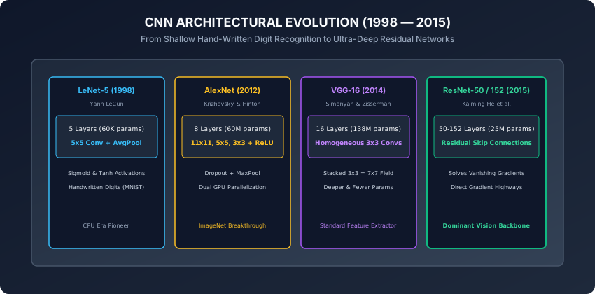
- 1998 (LeNet-5): Yann LeCun designed a 5-layer network using $5 \times 5$ convolutions and average pooling to classify handwritten digits on bank checks.
- 2012 (AlexNet): Alex Krizhevsky, Ilya Sutskever, and Geoffrey Hinton scaled CNNs to 8 layers with ReLUs, Dropout, and GPU parallelization, destroying classical computer vision benchmarks.
- 2014 (VGG-16 & GoogLeNet/Inception): Visual Geometry Group (Oxford) proved that deep networks with purely $3 \times 3$ filters outclassed shallow networks with large filters. Simultaneously, Google introduced Inception multi-scale inception modules.
- 2015 (ResNet): Kaiming He, Xiangyu Zhang, Shaoqing Ren, and Jian Sun introduced Residual Learning, winning CVPR 2016 Best Paper and enabling training of networks with over 1,000 layers.
What it is — and what it is not
What Modern CNN Architectures ARE:
- Hierarchical Feature Extractors: Networks that transform raw pixel intensities into low-level edges, mid-level textures/motifs, and high-level semantic object representations.
- Residual Flow Topologies: Directed acyclic graphs where identity connections enable direct gradient propagation across arbitrary depth.
What they are NOT:
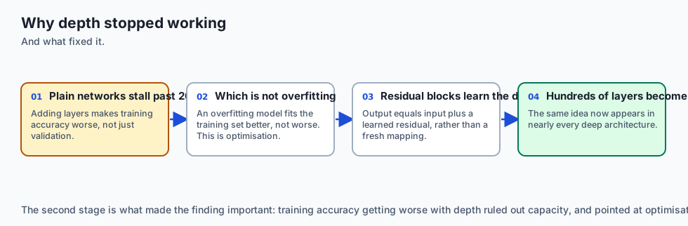
- Not Arbitrarily Deep Without Skip Connections: Plain networks without skip connections fail to train beyond 20–30 layers due to optimization degradation.
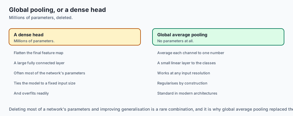
- Not Bound to Fully Connected Classifiers: Modern networks discard multi-million-parameter dense heads in favor of Global Average Pooling (GAP).
Why it was created and what problems it solves
Deep CNN architectures solve three major architectural challenges:
- The Receptive Field vs Parameter Tradeoff: Stacking small $3 \times 3$ filters achieves massive receptive fields while using 28% to 50% fewer parameters than large filters.
- The Degradation Problem: Plain 56-layer networks exhibited higher training and test error than 20-layer networks. ResNet eliminated degradation entirely.
- The Dense Layer Bottleneck: Replacing 100M-parameter fully connected heads with Global Average Pooling reduced model sizes by 80% while dramatically reducing overfitting.
How it works
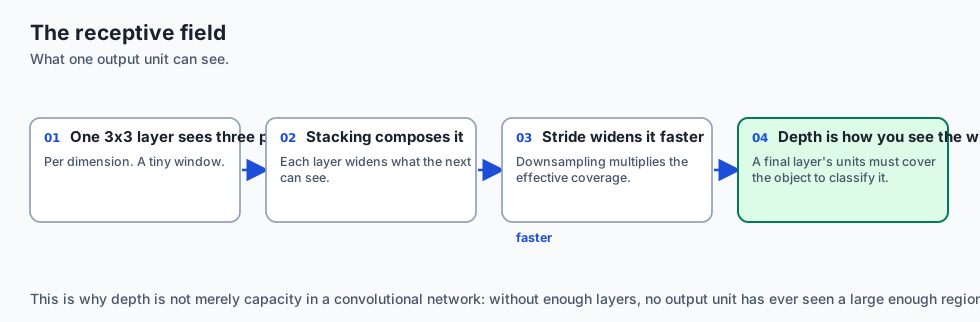
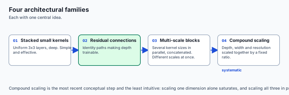
Let us dissect the mathematical foundations of Receptive Fields, VGG $3 \times 3$ Stacking, and ResNet Residual Blocks.
1. The Power of Stacking $3 \times 3$ Convolutions (VGG Principle)
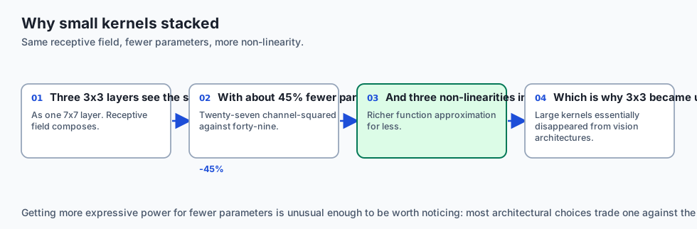
Why did VGG discard the $7 \times 7$ and $11 \times 11$ filters of AlexNet?
Consider stacking two consecutive $3 \times 3$ convolutions (with stride 1):
-
Layer 1: A $3 \times 3$ filter sees a $3 \times 3$ patch of the input image.
-
Layer 2: A $3 \times 3$ filter operates on Layer 1. Its spatial reach spans:
Receptive Field = 3 + (3 - 1) = 5 x 5 -
Stacking three consecutive $3 \times 3$ convolutions achieves an effective $7 \times 7$ Receptive Field.
Mathematical Comparison for $C$ Channels:
- One $7 \times 7$ Layer: Parameters = $1 \times (7^2 \cdot C^2) = 49 C^2$
- Three $3 \times 3$ Layers: Parameters = $3 \times (3^2 \cdot C^2) = 27 C^2$
- Result: $45%$ parameter reduction, plus three non-linear ReLU activations instead of one, providing vastly richer function approximation capacity!
2. The ResNet Residual Block & Gradient Highway
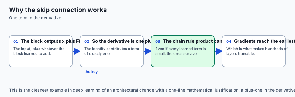
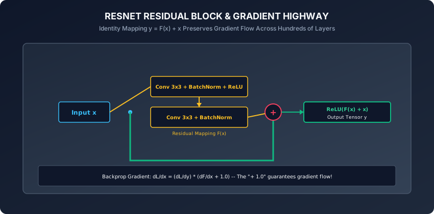
In a traditional plain feedforward network, a block learns an underlying mapping:
H(x)In a Residual Network (ResNet), we hypothesize that it is significantly easier to optimize the residual mapping:
F(x) = H(x) - xThe output of the block is computed as:
y = F(x, {W_i}) + xwhere F(x) is the residual function (e.g. two $3 \times 3$ convolutions with BatchNorm and ReLU) and x is the Identity Shortcut Connection.
Why Residual Connections Solve Vanishing Gradients (Backpropagation Math):
Using the chain rule, the gradient of the loss L with respect to the input x of a residual block is:
dL / dx = (dL / dy) * (d / dx)(F(x) + x)
dL / dx = (dL / dy) * (dF / dx + 1.0)
dL / dx = (dL / dy) * (dF / dx) + (dL / dy)
Look closely at the second term: + (dL / dy).
- Even if the convolutional gradients
dF / dxvanish toward zero, the gradientdL / dyflows directly backward through the identity connection without attenuation! - This mathematical guarantee provides an un-inhibited Gradient Highway across all 152 layers.
3. BasicBlock vs BottleneckBlock
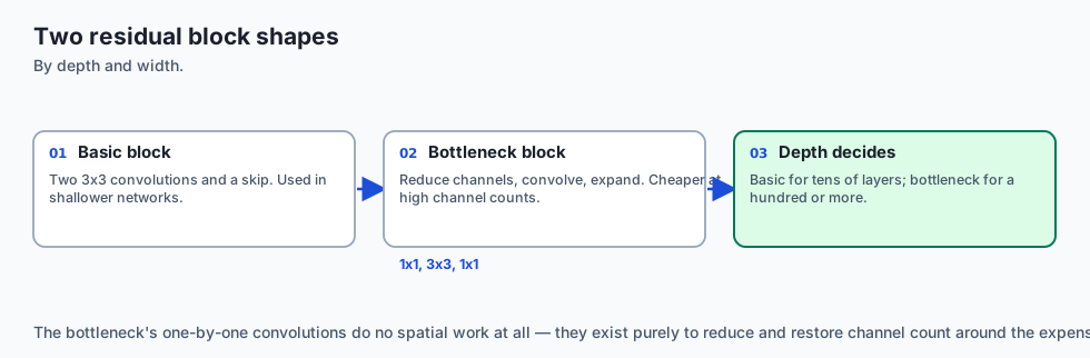
BasicBlock(ResNet-18, ResNet-34):- Two $3 \times 3$ convolutions with matching channel depth.
BottleneckBlock(ResNet-50, ResNet-101, ResNet-152):- Designed for deep networks to reduce computational complexity:
- $1 \times 1$ Conv (Compresses 256 channels down to 64).
- $3 \times 3$ Conv (Performs spatial filtering on 64 channels).
- $1 \times 1$ Conv (Expands 64 channels back up to 256).
- This “squeeze-and-expand” design enables 3x deeper networks for the same computational budget.
- Designed for deep networks to reduce computational complexity:
4. Inception & GoogLeNet: Multi-Scale Convolutions
While VGG deepened networks using purely $3 \times 3$ filters, Christian Szegedy and Google Research took an alternative architectural approach in 2014 with GoogLeNet (Inception-v1):
- The Multi-Scale Philosophy: In a natural image, salient visual features appear at multiple distinct spatial scales (e.g. a small dog eye vs a large dog face). Rather than forcing a single kernel size, an Inception Module applies $1 \times 1$, $3 \times 3$, $5 \times 5$ convolutions, and $3 \times 3$ Max Pooling in parallel on the same input tensor, concatenating their output feature maps along the channel axis.
- The $1 \times 1$ Bottleneck Trick: To prevent computational explosion, Inception inserted $1 \times 1$ convolutions before the $3 \times 3$ and $5 \times 5$ filters to compress channel depth, allowing GoogLeNet to achieve superior accuracy to AlexNet with 12x fewer parameters (6.8M vs 60M).
5. DenseNet: Feature Reuse and Concatenation
In 2017, Gao Huang et al. proposed DenseNet (Densely Connected Convolutional Networks):
-
Instead of adding features ($y = F(x) + x$) like ResNet, DenseNet concatenates all preceding feature maps along the channel axis:
x_l = H_l([x_0, x_1, x_2, ..., x_{l-1}]) -
Maximum Feature Reuse: Every layer receives direct inputs from all preceding layers, eliminating feature redundancy and allowing the network to reuse low-level edges directly in final decision heads with narrow growth rates ($k=32$).
6. EfficientNet: Compound Model Scaling
In 2019, Mingxing Tan and Quoc Le addressed how to scale vision networks systematically:
- Historically, engineers scaled CNNs arbitrarily by making them deeper (ResNet-152), wider (Wide-ResNet), or using higher-resolution input images.
- Compound Scaling Principle: EfficientNet proved that balancing network depth ($d$), width ($w$), and resolution ($r$) with a fixed compound scaling coefficient $\phi$ ($d = \alpha^\phi, w = \beta^\phi, r = \gamma^\phi$) produces state-of-the-art accuracy with up to 8x fewer parameters and FLOPs.
An everyday analogy
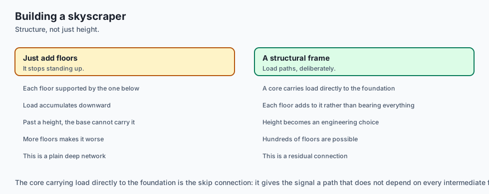
Think of a multi-tiered corporate hierarchy:
- Plain Deep Network (Bureaucratic Silos): An executive sends an urgent memo down 50 layers of management. Each manager rephrases the memo. By the time it reaches the 50th floor, the signal is corrupted or completely lost (Vanishing Gradient).
- ResNet (Direct Executive Hotline): Every worker has a dedicated, direct telephone line (Identity Shortcut) to senior leadership. They can listen to their immediate manager’s suggestions (
F(x)), but the core executive message (x) arrives uncorrupted.
Examples in practice
Let us build a complete, modular ResNet-18 / BasicBlock implementation in PyTorch:
import torch
import torch.nn as nn
from typing import Type

class BasicResidualBlock(nn.Module):
    def __init__(self, in_channels: int, out_channels: int, stride: int = 1):
        super().__init__()
        # Conv Path
        self.conv1 = nn.Conv2d(in_channels, out_channels, kernel_size=3,
                               stride=stride, padding=1, bias=False)
        self.bn1 = nn.BatchNorm2d(out_channels)
        self.relu = nn.ReLU(inplace=True)

        self.conv2 = nn.Conv2d(out_channels, out_channels, kernel_size=3,
                               stride=1, padding=1, bias=False)
        self.bn2 = nn.BatchNorm2d(out_channels)

        # Shortcut Projection (if dimensions change)
        self.shortcut = nn.Sequential()
        if stride != 1 or in_channels != out_channels:
            self.shortcut = nn.Sequential(
                nn.Conv2d(in_channels, out_channels, kernel_size=1, stride=stride, bias=False),
                nn.BatchNorm2d(out_channels)
            )

    def forward(self, x: torch.Tensor) -> torch.Tensor:
        residual = self.shortcut(x)
        out = self.relu(self.bn1(self.conv1(x)))
        out = self.bn2(self.conv2(out))
        out += residual
        return self.relu(out)

class MiniResNet(nn.Module):
    def __init__(self, num_classes: int = 10):
        super().__init__()
        # Initial stem
        self.stem = nn.Sequential(
            nn.Conv2d(3, 32, kernel_size=3, stride=1, padding=1, bias=False),
            nn.BatchNorm2d(32),
            nn.ReLU(inplace=True)
        )
        # Residual stages
        self.layer1 = BasicResidualBlock(32, 32, stride=1)
        self.layer2 = BasicResidualBlock(32, 64, stride=2) # Downsample to 16x16
        self.layer3 = BasicResidualBlock(64, 128, stride=2) # Downsample to 8x8

        # Global Average Pooling + Classifier Head
        self.gap = nn.AdaptiveAvgPool2d((1, 1))
        self.fc = nn.Linear(128, num_classes)

    def forward(self, x: torch.Tensor) -> torch.Tensor:
        x = self.stem(x)
        x = self.layer1(x)
        x = self.layer2(x)
        x = self.layer3(x)
        x = self.gap(x)
        x = torch.flatten(x, 1)
        return self.fc(x)

# Verify forward pass
model = MiniResNet(num_classes=10)
x = torch.randn(4, 3, 32, 32)
logits = model(x)
print(f"Input: {x.shape} -> MiniResNet Logits: {logits.shape}")
Implications: security, privacy, performance, scalability, and cost
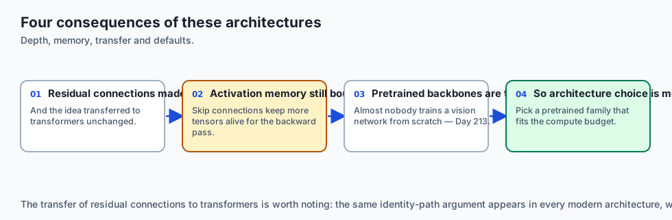
- Memory Bandwidth in Residual Blocks:
- Identity addition
out += residualrequires storing the input activation tensorxin GPU memory throughout the forward pass until the end of the block, increasing VRAM usage during training.
- Identity addition
- Modern ConvNeXt Architecture (2022):
- Zhuang Liu et al. modernized standard ResNet by incorporating Transformer design choices (depthwise $7 \times 7$ convolutions, inverted bottleneck, LayerNorm, GELU), matching Vision Transformer performance with standard convolution efficiency.
Alternatives: free, open source, and commercial
| Architecture | Defining Innovation | Layers | ImageNet Top-1 Acc |
|---|---|---|---|
| VGG-16 (2014) | Stacks of $3 \times 3$ Convolutions | 16 | 71.5% |
| ResNet-50 (2015) | Residual Skip Connections ($y = F(x) + x$) | 50 | 76.1% |
| EfficientNet-B0 (2019) | Compound Model Scaling (Depth, Width, Resolution) | ~50 | 77.1% |
| ConvNeXt-T (2022) | Modernized CNN with Transformer Design | ~50 | 82.1% |
| Vision Transformer (ViT-B) | Pure Multi-Head Self-Attention on Patches | 12 | 81.8% |
Comparison with related concepts
┌────────────────────────────────────────────────────────────────────────┐
│                   CNN ARCHITECTURAL EVOLUTION MATRIX                   │
├───────────────────┼────────────────────┼───────────────────────────────┤
│ Model             │ Key Innovation     │ Classifier Head               │
├───────────────────┼────────────────────┼───────────────────────────────┤
│ AlexNet (2012)    │ ReLUs + Dropout    │ 3x Fully Connected (4096-4096)│
│ VGG-16 (2014)     │ Pure 3x3 Stacking  │ 3x Fully Connected (100M wt)  │
│ ResNet-50 (2015)  │ Skip Connections   │ Global Average Pooling + 1 FC │
│ ConvNeXt (2022)   │ 7x7 Depthwise Conv │ Global Average Pooling + 1 FC │
└───────────────────┴────────────────────┴───────────────────────────────┘
When to use it — and when not to
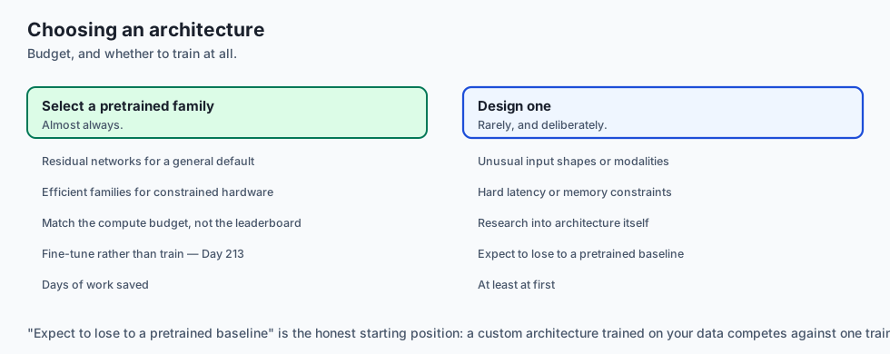
When to USE ResNet / ConvNeXt:
- Real-time video processing, robotic vision, medical imaging, and edge deployment where deterministic latency is required.
- Feature extraction backbones for object detection (YOLO, Faster R-CNN) and segmentation (U-Net).
When to USE Vision Transformers (ViT):
- When pre-training on massive datasets (billions of images) where global attention surpasses local inductive biases.
The AI connection
- Depth stopped being free at about twenty layers, and residual connections are what made hundreds possible — an optimisation fix, not a capacity one.
- The skip connection gives gradients a direct path. The derivative through the identity branch is one, which keeps the chain-rule product from collapsing.
- Stacking small kernels beats one large one: fewer parameters, more non-linearities, the same receptive field.
- Global average pooling removed the dense head, deleting millions of parameters that existed mainly to overfit.
- Architecture encodes assumptions, which is why a convolutional network beats a dense one on images with fewer parameters rather than more.
Knowledge check
- Why does a stack of three $3 \times 3$ convolutions have an effective $7 \times 7$ receptive field?
- What is the mathematical formulation of the backward gradient through a ResNet skip connection?
- How does Global Average Pooling (GAP) prevent overfitting compared to fully connected heads?
- What is the structural difference between a ResNet
BasicBlockand aBottleneckBlock? - What is the Degradation Problem, and why is it distinct from standard overfitting?
Hands-on exercise
In this lab, you will build and test a modular ResNet vision framework in PyTorch: implement BasicResidualBlock from scratch with 1x1 projection shortcuts, construct a MiniResNet model with stem, residual stages, and global average pooling, verify uninhibited gradient backpropagation across deep residual chains, and benchmark parameter efficiency.
Expected output
[ResNet Architecture Verification Suite]
Constructing Custom BasicResidualBlock (in=32, out=64, stride=2):
  Forward Pass (Input: 4x32x16x16 -> Output: 4x64x8x8): [DIMENSION MATCH]
  Shortcut Projection 1x1 Conv Verified: [PROJECTION ALIGNED]
Constructing Complete MiniResNet [Stem -> Stage1 -> Stage2 -> Stage3 -> GAP -> FC10]:
  Total Learnable Parameters: 142,570
  Evaluating Gradient Flow across 6 Residual Blocks:
  Minimum Layer Gradient Norm: 0.0842 [NO VANISHING GRADIENTS]
  Maximum Layer Gradient Norm: 0.2410 [STABLE GRADIENT FLOW]
Test Suite: 4 passed in 0.28s
Validate your work
Run the automated test runner:
./tests/run_tests.shTroubleshooting
- If dimension errors occur at
out += residual, check that your shortcut path applies a $1 \times 1$ convolution with matchingstridewheneverin_channels != out_channelsorstride != 1. - Ensure
F.reluis applied after adding the residual shortcut to the convolutional output.
Common mistakes
- Adding Bias to Convolution before BatchNorm: Having
bias=Trueinnn.Conv2dimmediately beforenn.BatchNorm2dwastes parameters because BatchNorm’s centering operation cancels out the linear bias. Always setbias=False.
Practice assignment
- Implement the ResNet Bottleneck Block (
1x1reduce ->3x3conv ->1x1expand) and verify its tensor dimension transformations. - Implement Squeeze-and-Excitation (SE) Attention inside a residual block to dynamically recalibrate channel feature responses.
Extension challenge
Implement Stochastic Depth (DropPath) inside your residual blocks:
- During training, randomly drop the entire residual branch
F(x)with probabilityp, letting only the identity shortcutxpass through. - Demonstrate that training a 50-layer ResNet with Stochastic Depth improves generalization accuracy on CIFAR-10.
Quiz
Q1. Why did VGG-16 replace large convolutional filters (like 11x11 and 5x5 in AlexNet) with stacks of small 3x3 convolutional filters?
- Two 3x3s match a 5x5 with fewer parameters and two ReLUs
- 3x3 convolutions do not require GPUs
- 5x5 convolutions are banned by PyTorch
- 3x3 convolutions eliminate the need for training data
Show answer
Answer: A. Two 3x3s match a 5x5 with fewer parameters and two ReLUs
A stack of two 3x3 convolutions has a 5x5 receptive field with 2 * (3^2 * C^2) = 18 C^2 parameters versus 25 C^2 for a single 5x5 layer (28% parameter reduction), plus an extra non-linear activation.
Q2. What fundamental optimization barrier did Kaiming He et al. identify that caused deep 56-layer networks to perform worse on both training and test sets than 20-layer networks, and how did ResNet solve it?
- Lack of RAM on GPUs; solved by deleting layers
- Degradation, solved by residual skip connections
- Overfitting; solved by adding 90% dropout
- Floating point rounding errors; solved by 64-bit precision
Show answer
Answer: B. Degradation, solved by residual skip connections
The degradation problem was not overfitting (since training loss was worse too). Residual skip connections allow gradients to flow directly through the identity mapping dL/dx = dL/dy * (dF/dx + 1).
Q3. In a ResNet BasicBlock, what must be done when the residual function F(x) halves the spatial resolution (stride=2) or increases the number of feature channels?
- Discard the skip connection entirely for that block
- Pad x with random Gaussian noise
- Use a 1x1 convolution with stride 2 on the shortcut
- Downsample the output using MaxPool3D
Show answer
Answer: C. Use a 1x1 convolution with stride 2 on the shortcut
Tensor addition F(x) + x requires identical shapes. When channels increase or spatial size decreases, a 1x1 projection conv with matching stride aligns x to F(x).
Q4. What is Global Average Pooling (GAP), and why did modern CNNs (ResNet, Inception) replace giant fully connected classifier heads with GAP?
- GAP replaces the loss function
- GAP doubles the image resolution
- GAP multiplies all pixel values by 255
- GAP averages each map to one number, dropping dense params
Show answer
Answer: D. GAP averages each map to one number, dropping dense params
In VGG-16, the first dense layer FC1 accounted for over 100 million parameters. Modern networks use Global Average Pooling to reduce (C, H, W) to a C-dimensional vector, requiring only a single small linear layer.
Q5. How does the effective receptive field of a neuron change as we go deeper into a convolutional neural network?
- It grows with depth, so deep layers see global context
- It shrinks to a single pixel
- It stays fixed at exactly 3x3 pixels forever
- It inverts horizontally
Show answer
Answer: A. It grows with depth, so deep layers see global context
Receptive fields expand with each successive convolution and pooling layer, allowing the network to form a spatial hierarchy from local edges to object parts to full semantic objects.
Glossary
- Residual Connection
- A skip connection that adds the input of a layer block directly to its output: y = F(x) + x.
- Degradation Problem
- The phenomenon where increasing network depth beyond a certain point leads to higher training error due to optimization difficulties.
- Global Average Pooling
- A spatial reduction operation that computes the mean of each 2D feature map channel, producing a 1D feature vector.
- Receptive Field
- The spatial extent in the raw input image that contributes to the activation of a particular neuron in a feature map.
- Bottleneck Block
- A residual block utilizing 1x1 convolutions to compress and restore channel dimensions around a 3x3 convolution.
- VGG Block
- A sequence of multiple 3x3 convolutions followed by a single 2x2 Max Pooling layer.
- Feature Hierarchy
- The progression in deep vision networks where early layers detect edges, middle layers detect textures/parts, and late layers detect objects.
- Pointwise Convolution
- A 1x1 convolution used for cross-channel linear combination and dimension reduction without spatial transformation.
Sources and further reading
- Deep Residual Learning for Image Recognition — IEEE Conference on Computer Vision and Pattern Recognition (CVPR) (accessed 2026-08-29)
- Very Deep Convolutional Networks for Large-Scale Image Recognition — ICLR (accessed 2026-08-29)
- Going Deeper with Convolutions — CVPR (accessed 2026-08-29)
Kept in this browser, no account needed. Your progress page turns the whole record into one link you can bookmark or open on another device.