Deep Learning › Training at Scale › Day 234
Day 234: Distributed Training Concepts
Master distributed training architectures and scaling paradigms: compare DDP vs DP, analyze Ring-AllReduce collective communications, understand ZeRO memory stages (ZeRO-1, ZeRO-2, ZeRO-3 / PyTorch FSDP), master 3D Parallelism (Tensor Parallelism Megatron-LM, Pipeline Parallelism 1F1B schedule, and Sequence Parallelism), diagnose communication-to-computation overlap, and simulate distributed rank synchronization in PyTorch.
Hands-on lab for this lesson
Lab files on GitHub: https://github.com/ai-roadmap-365/ai-roadmap-365.github.io/tree/main/labs/sections/deep-learning/day-234-distributed-training-concepts
- Get the hands-on files. Clone the labs repository once (you can reuse this clone for every lesson). This works on macOS, Linux, and Windows (PowerShell or WSL):
git clone https://github.com/ai-roadmap-365/ai-roadmap-365.github.io.git cd ai-roadmap-365.github.io - Open this lesson's lab. Move into the directory for this specific day. Every lab lives at the same predictable path — section / subsection / week / day:
cd labs/sections/deep-learning/day-234-distributed-training-concepts - Read the lab guide. Open `README.md` in that directory. It lists the exact commands, what each does, the expected output, and how to check your work — read it before running anything.
- Run it and check your work. Follow the README's "How to run" section: run the example first to see the finished result, then complete the numbered exercises in `starter/`, then run the tests. The tests pass (exit 0) only when your work is correct.
bash tests/run_tests.sh # or the test command named in the lab README
You can also open the lab as a local page (works offline, shows the file tree and expected output).
Learning objectives
By the end of this lesson you will be able to:
- Compare PyTorch DataParallel (DP) single-process multi-threading with DistributedDataParallel (DDP) multi-process ring communication.
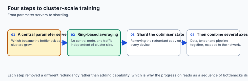
- Derive the Ring-AllReduce collective communication algorithm and its bandwidth optimality (2 * (N - 1) / N * Data).
- Analyze ZeRO memory partitioning stages (ZeRO-1, ZeRO-2, ZeRO-3) and PyTorch Fully Sharded Data Parallel (FSDP).
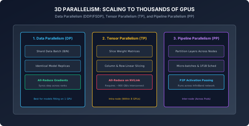
- Explain 3D Parallelism: Tensor Parallelism (TP column/row linear slicing) and Pipeline Parallelism (PP 1F1B schedule).
- Simulate distributed rank communication and Ring-AllReduce aggregation in Python.
Prerequisites
Why this matters
A single modern GPU (such as an NVIDIA H100 with 80 GB VRAM) is an engineering marvel.
Yet, a 70-Billion parameter LLaMA model in mixed precision requires over 1,120 GB of VRAM just for static training states (weights, gradients, optimizer moments), completely blowing past the physical memory limit of any single chip on Earth.
To train frontier models, we must distribute computation across clusters of thousands of GPUs:
- How do 1,024 GPUs stay in perfect mathematical synchrony without spending
90\%of their time waiting on network cables? - How does DeepSpeed ZeRO / PyTorch FSDP shatter the memory barrier by sharding weights across nodes?
- How does Megatron-LM Tensor Parallelism slice a single matrix multiplication across 8 GPUs over 900 GB/s NVLink fabrics?
Today, you will master the principles of Distributed Data Parallelism (DDP), the Ring-AllReduce algorithm, ZeRO Memory Sharding (FSDP), and 3D Parallelism.
The idea in plain language
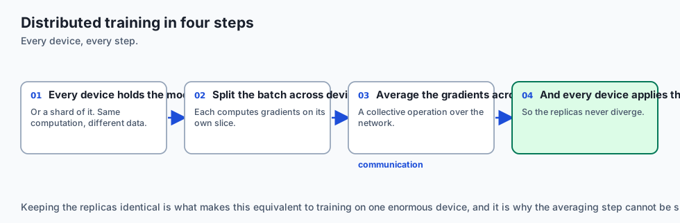
Think of constructing a 100-story skyscraper:
- Single GPU (One Solo Builder): One person trying to pour concrete, install plumbing, and wire electrical panels alone. They run out of physical carrying capacity (Out of Memory) and the build takes 500 years.
- Data Parallelism (100 Duplicate Construction Teams): 100 identical teams building 100 separate identical suburban homes simultaneously (Sharded Data Batches). At the end of each day, they meet on a radio channel to agree on the revised blueprints (All-Reduce Gradients).
- Tensor Parallelism (8 Specialists Lifting One Steel Beam): 8 workers simultaneously lifting and welding a massive 10-ton steel girder that no individual worker could lift alone (Slicing Matrix Projections on NVLink).
- Pipeline Parallelism (Assembly Line Floors): Team A builds Floor 1
\rightarrowpasses to Team B for Floor 2\rightarrowpasses to Team C for Floor 3 (1F1B Layer Partitioning).
Historical background
- 2017 (Baidu & Ring-AllReduce): Andrew Gibiansky and Baidu Research brought Ring-AllReduce from High Performance Computing (HPC) into deep learning, demonstrating linear scaling across 128 GPUs.
- 2019 (NVIDIA & Megatron-LM): Shoeybi et al. published Tensor Parallelism, enabling intra-node matrix slicing with minimal communication overhead.
- 2019 (Microsoft DeepSpeed & ZeRO): Rajbhandari et al. introduced the Zero Redundancy Optimizer, proving that memory redundancy could be eliminated without the complexity of pipeline partitioning.
- 2023 (Meta AI & PyTorch FSDP): Productionized Fully Sharded Data Parallel natively in PyTorch core, making trillion-parameter distributed scaling accessible to all engineers.
What it is — and what it is not
What Distributed Training IS:
- Multi-Process Architecture: Independent OS processes running across separate GPUs communicating via NCCL (NVIDIA Collective Communications Library).
- Asynchronous Compute-Communication Overlap: Commencing gradient All-Reduce on later layers while earlier layers are still computing backward passes.
What it is NOT:
- Not Python Multi-Threading: Python threading is bottlenecked by the Global Interpreter Lock (GIL). Distributed deep learning uses independent operating system processes per GPU via
torch.distributed.
Why it was created and what problems it solves
Distributed training solves two fundamental scaling barriers:
- The Throughput Barrier (Dataset Scale): Pretraining an LLM on 15 Trillion tokens on 1 GPU would take 150 years. With 1,024 GPUs in Data Parallelism, training completes in 50 days.
- The Memory Capacity Barrier (Model Size): Storing a 405B parameter model requires 6.5 TB of VRAM. Distributed sharding (FSDP / Tensor Parallelism) splits the model across hundreds of chips.
How it works
Let us dissect collective communications, DDP mechanics, ZeRO stages, and 3D parallelism.
1. The Ring-AllReduce Algorithm (Baidu, 2017)
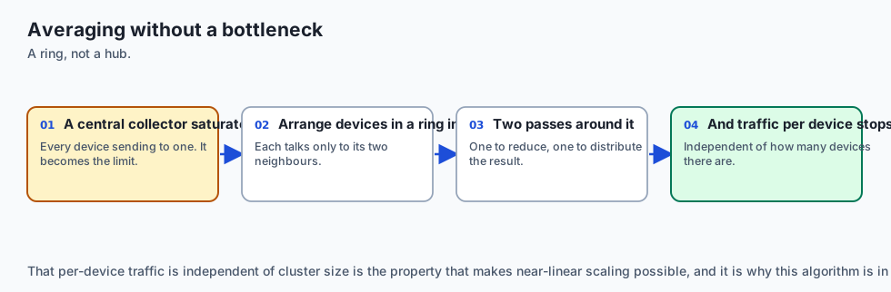
How do P GPUs compute the average of their gradient tensors of size V without a central master bottleneck?
In Ring-AllReduce, the P GPUs are arranged in a logical unidirectional ring (0 \rightarrow 1 \rightarrow 2 \rightarrow \dots \rightarrow P-1 \rightarrow 0):
- Step 1: Scatter-Reduce (
P - 1steps):- Each GPU divides its gradient tensor into
Pequal chunks. - At each step, GPU
isends chunkkto GPUi+1and receives chunkk-1from GPUi-1, summing received data into its local chunk. - After
P-1steps, each GPU holds the exact global sum of one distinct chunk of the gradient tensor!
- Each GPU divides its gradient tensor into
- Step 2: All-Gather (
P - 1steps):- Each GPU sends its fully reduced chunk around the ring.
- After
P-1steps, every GPU holds the complete, globally reduced gradient tensor!
Bandwidth Optimality:
\text{Total Data Transferred per GPU} = 2 \times \left(\frac{P - 1}{P}\right) \times V- As
P \rightarrow \infty, data transferred per GPU is bounded by2V(independent of cluster size!), achieving near-linear scaling!
2. PyTorch DistributedDataParallel (DDP)
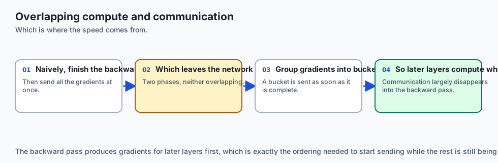
In DDP:
- Each GPU runs an identical model replica on a dedicated process.
- Gradient Bucketing & Overlapping: DDP groups parameter gradients into contiguous memory buffers (Buckets, typically 25 MB).
- As soon as a bucket fills during the backward pass, DDP immediately launches an asynchronous non-blocking
All-Reducecollective over NCCL while the GPU continues backpropagating earlier layers!
3. ZeRO Memory Sharding & PyTorch FSDP
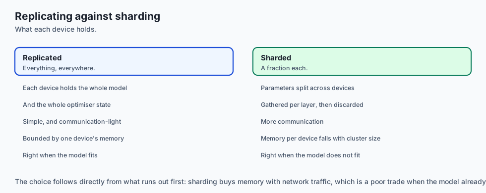
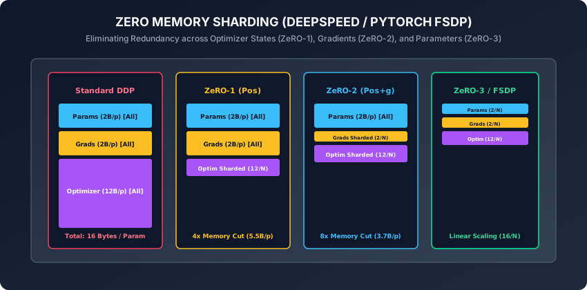
In standard DDP, every GPU redundantly holds identical model parameters, gradients, and optimizer states (16 \text{ Bytes / Parameter}).
ZeRO (Zero Redundancy Optimizer) eliminates this redundancy in three progressive stages:
┌────────────────────────────────────────────────────────────────────────┐
│                   ZERO / FSDP SHARDING STAGES                          │
├──────────────┬────────────────────────┬───────────────┬────────────────┤
│ Stage        │ Sharded Components     │ Memory / Param│ Comm Overhead  │
├──────────────┼────────────────────────┼───────────────┼────────────────┤
│ Baseline DDP │ None (Full Redundancy) │ 16 Bytes      │ 0% Baseline    │
│ ZeRO-1 (Pos) │ Optimizer States Only  │ 4 + 12/P Bytes│ 0% Overhead    │
│ ZeRO-2 (Pos+g│ Optimizer + Gradients  │ 2 + 14/P Bytes│ 0% Overhead    │
│ ZeRO-3 / FSDP│ Optim + Grads + Params │ 16/P Bytes    │ +50% AllGather │
└──────────────┴────────────────────────┴───────────────┴────────────────┘
How ZeRO-3 / FSDP Operates at Runtime:
- Forward Pass: Before executing layer
L, the GPUs perform anAll-Gatherto temporarily reconstruct the full weights of layerL. The layer executes, and the full weights are immediately deleted from VRAM, keeping only the1/Plocal shard! - Backward Pass: Before computing gradients for layer
L, anotherAll-Gatherreconstructs full weights. Gradients are computed, reduced across ranks viaReduce-Scatter, and full weights are deleted again!
4. 3D Parallelism: Megatron-LM Tensor & Pipeline Parallelism
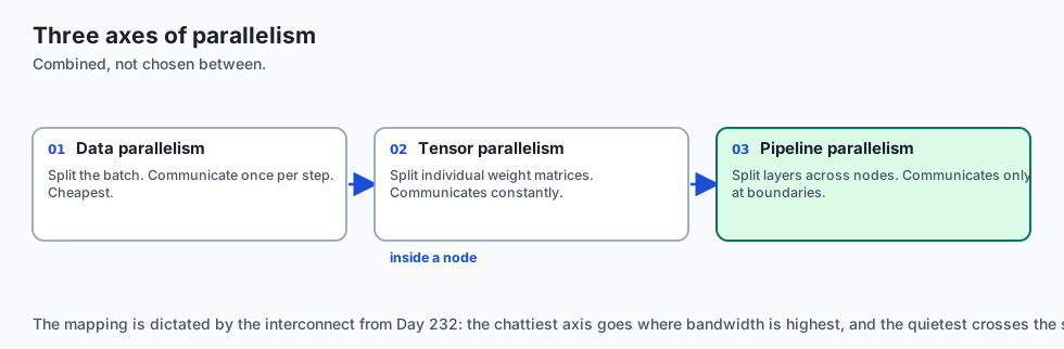
For models exceeding 100B parameters, combining DP, TP, and PP yields 3D Parallelism:
A. Tensor Parallelism (TP / Megatron-LM):
- Slices the internal weight matrices of Transformer layers:
- Self-Attention QKV Projections: Column-parallel split (
W_Q = [W_{Q1} \mid W_{Q2}]). - Attention Output Projection: Row-parallel split (
W_O = [W_{O1}^\top \mid W_{O2}^\top]^\top).
- Self-Attention QKV Projections: Column-parallel split (
- Only requires one All-Reduce at the end of Attention and one All-Reduce at the end of MLP!
- Placed within an 8-GPU NVLink node due to high communication frequency.
B. Pipeline Parallelism (PP / 1F1B Schedule):
- Partitions the 80 layers of a Transformer across 8 separate nodes (10 layers per node).
- Uses 1F1B (One-Forward-One-Backward) schedule: Each GPU alternates 1 forward step with 1 backward step on micro-batches, capping activation memory and keeping pipeline bubbles under
10\%.
5. Sequence Parallelism & DeepSpeed Ulysses (Korthikanti et al., 2022)
In standard Tensor Parallelism, LayerNorm and Dropout activations are still duplicated across all TP ranks:
- Sequence Parallelism (SP): Splits activations along the sequence length dimension (
L / P) during LayerNorm and Dropout, eliminating duplicate activation memory. - DeepSpeed Ulysses: Utilizes an
All-to-Allcollective communication primitive to transpose tokens from Sequence-sharded to Head-sharded before attention, enabling million-token context training with minimal communication overhead!
6. Context Parallelism & RingAttention (Liu et al., 2023)
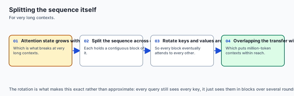
How do modern models process 1,000,000+ token context windows without crashing GPU VRAM?
- RingAttention: Distributes the sequence across a ring of GPUs.
- Each GPU holds a chunk of queries
Q_i, and passes key-value blocksK_j, V_jaround the ring in overlapping communication-computation cycles, computing exact global self-attention across arbitrary sequence lengths without ever storing the fullN \times Nattention matrix on any single device!
7. Expert Parallelism in Mixture-of-Experts (MoE / Lepikhin et al., GShard)
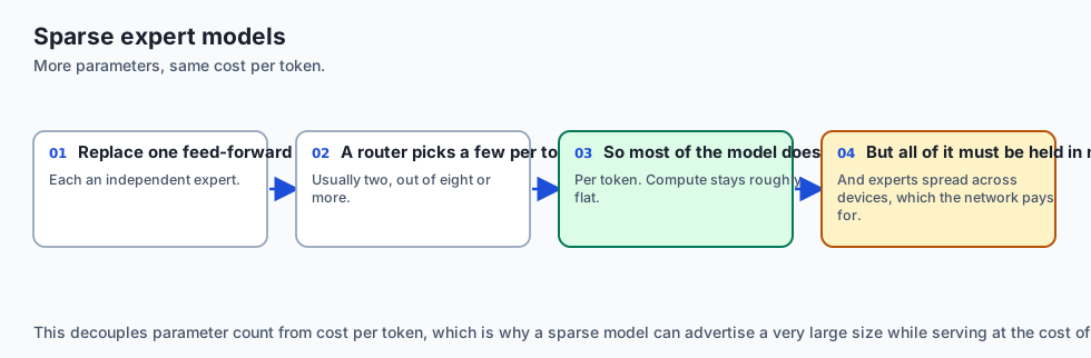
In sparse Mixture-of-Experts models (like Mixtral 8x7B or Grok-1):
- Expert Parallelism (EP): Different GPUs host different Feed-Forward Expert networks.
- A Router / Gate Network routes individual tokens to top-
kexperts across the cluster usingAll-to-Alldispatch and combine collectives. - Allows scaling parameter capacity to hundreds of billions of parameters while keeping compute FLOPs per token constant!
8. Production Cluster Orchestration: torchrun and NCCL Tuning
To launch distributed jobs reliably on production clusters:
-
torchrun: The official PyTorch elastic launcher managing environment variables (RANK,WORLD_SIZE,LOCAL_RANK,MASTER_ADDR,MASTER_PORT). -
NCCL Tuning Flags:
export NCCL_DEBUG=INFO export NCCL_IB_DISABLE=0 # Enable InfiniBand RDMA export NCCL_NET_GDR_LEVEL=5 # Enable GPUDirect RDMA export TORCH_DISTRIBUTED_DEBUG=DETAIL -
PyTorch 2.x DeviceMesh: A high-level abstraction defining 2D and 3D GPU grids for orchestrating hybrid parallel configurations (e.g., FSDP across nodes and Tensor Parallelism within nodes) cleanly and declaratively. This provides fine-grained control over multi-dimensional collective communication groups.
An everyday analogy
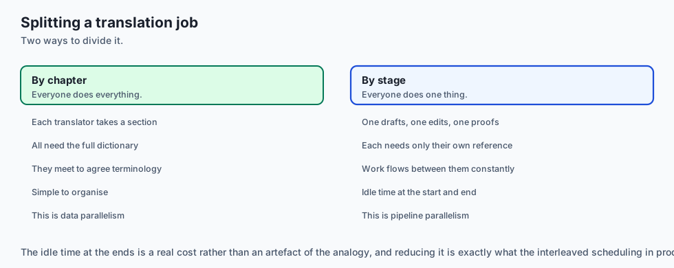
Think of translating an encyclopedic 1,000-page book from English to Spanish:
- Data Parallelism: 10 translators. Each translator gets 100 distinct chapters. They translate independently, and meet weekly to synchronize style and terminology (Ring-AllReduce).
- Tensor Parallelism: 4 translators sitting at the same table working on the exact same complex sentence simultaneously, splitting idioms and grammar at high conversational speed (NVLink Intra-Node).
- Pipeline Parallelism: An assembly line where Translator 1 translates draft
\rightarrowEditor 2 polishes grammar\rightarrowTypesetter 3 formats pages (1F1B Micro-Batches).
Examples in practice
Let us build a Simulated Ring-AllReduce Collective Communication Engine in Python:
import numpy as np
from typing import List

def ring_allreduce_simulation(rank_tensors: List[np.ndarray]) -> List[np.ndarray]:
    # Simulates the Ring-AllReduce collective communication algorithm across P ranks.
    P = len(rank_tensors)
    assert P > 1, "Ring-AllReduce requires at least 2 ranks."
    tensor_len = len(rank_tensors[0])
    assert tensor_len % P == 0, f"Tensor length {tensor_len} must be divisible by {P}"
    chunk_size = tensor_len // P

    # Make working copies: list of P chunks per rank
    ranks = [[t[i*chunk_size:(i+1)*chunk_size].copy() for i in range(P)] for t in rank_tensors]

    # 1. Scatter-Reduce Phase (P - 1 steps)
    for step in range(P - 1):
        for r in range(P):
            send_chunk_idx = (r - step) % P
            recv_chunk_idx = (r - step - 1) % P
            send_val = ranks[r][send_chunk_idx]
            recv_rank = (r + 1) % P
            # Add received chunk to next rank
            ranks[recv_rank][send_chunk_idx] += send_val

    # 2. All-Gather Phase (P - 1 steps)
    for step in range(P - 1):
        for r in range(P):
            send_chunk_idx = (r - step + 1) % P
            send_val = ranks[r][send_chunk_idx]
            recv_rank = (r + 1) % P
            ranks[recv_rank][send_chunk_idx] = send_val.copy()

    # Reassemble full tensors for each rank
    return [np.concatenate(r) for r in ranks]
Implications: security, privacy, performance, scalability, and cost
- Network Fault Tolerance & Stragglers:
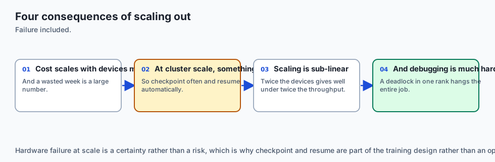
- In synchronous DDP, if a single GPU among 1,024 throttles due to heat or a degraded optical cable, all 1,023 other GPUs stall on the All-Reduce barrier. Continuous telemetry (NCCL health checks) is essential.
- Gradient Inversion & Differential Privacy:
- In federated distributed training, transmitting unencrypted raw gradients can allow adversaries to reconstruct private training images or text via gradient inversion attacks.
Alternatives: free, open source, and commercial
| Distributed Framework | Primary Technology | Scaling Range | Best Use Case |
|---|---|---|---|
| PyTorch DDP | Multi-Process All-Reduce | 2 - 128 GPUs | Models fitting on 1 GPU |
| PyTorch FSDP | Native ZeRO-3 Sharding | 8 - 1,024 GPUs | Models 7B - 70B params |
| DeepSpeed (ZeRO) | ZeRO-1/2/3 + Offload | 8 - 4,096 GPUs | Trillion-param training |
| Megatron-Core | 3D Parallelism (TP+PP+DP) | 64 - 100,000 GPUs | Frontier LLM Pretraining |
Comparison with related concepts
┌────────────────────────────────────────────────────────────────────────┐
│                   DISTRIBUTED PARADIGMS COMPARISON                     │
├────────────────────┬─────────────────┬──────────────────┬──────────────┤
│ Paradigm           │ What is Sharded │ Interconnect Req │ Comm Volume  │
├────────────────────┼─────────────────┼──────────────────┼──────────────┤
│ DDP                │ Data Batch      │ Low (InfiniBand) │ 2 * Grads    │
│ FSDP / ZeRO-3      │ Data + Weights  │ Moderate (RoCE)  │ 3 * Weights  │
│ Tensor Parallel (TP│ Weight Matrices │ Ultra-High(NVLink│ 2x / Layer   │
│ Pipeline (PP)      │ Network Layers  │ Low (P2P Stream) │ Activations  │
└────────────────────┴─────────────────┴──────────────────┴──────────────┘
When to use it — and when not to
When to Use Distributed Training:
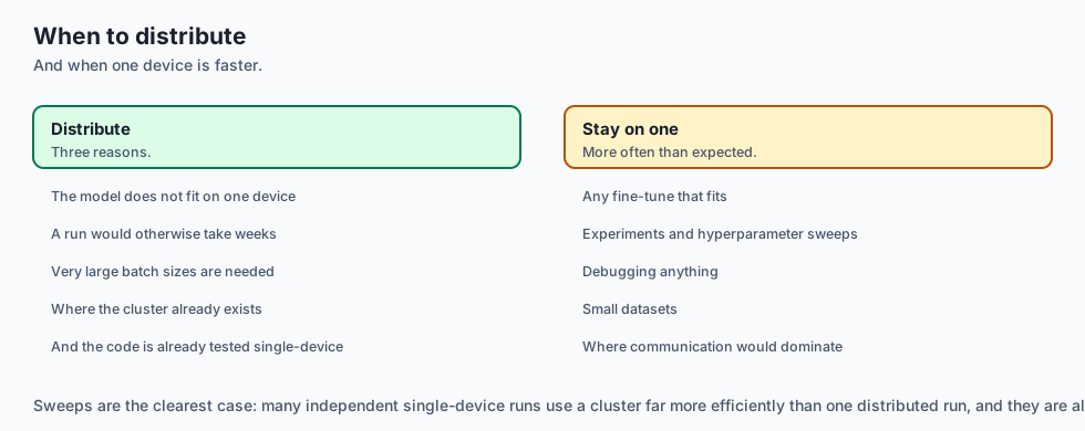
- Model parameters exceed single-GPU VRAM capacity, dataset size requires multi-GPU throughput, or training time must be compressed from months to days.
When NOT to use:
- Small models (<1B parameters) on small datasets where network synchronization overhead exceeds computation time.
The AI connection
- Every frontier model is trained on a cluster, so distribution is not an advanced topic but the ordinary condition of large-scale training.
- Communication cost, not compute, limits scaling, which is why the collective algorithms matter as much as the accelerators.
- Sharding made trillion-parameter models trainable by removing the requirement that each device hold a full copy of everything.
- Parallelism is combined along several axes at once — data, tensor, pipeline — and the mapping to network topology is a first-order design decision.
- Sparse expert models scale capacity without scaling cost per token, which changes the economics of very large models.
Knowledge check
- What is the fundamental difference between PyTorch DP and PyTorch DDP?
- How does Ring-AllReduce achieve constant per-GPU communication volume independent of cluster size?
- What are the differences between ZeRO-1, ZeRO-2, and ZeRO-3 memory sharding?
- Why is Tensor Parallelism typically restricted to an 8-GPU NVLink node rather than running across nodes?
- How does the 1F1B schedule reduce the pipeline bubble in Pipeline Parallelism?
Hands-on exercise
In this lab, you will build and test a modular distributed training simulation engine in Python: implement Ring-AllReduce collective communication mechanics, calculate ZeRO memory sharding budgets across cluster ranks, simulate gradient aggregation across distributed processes, and verify mathematical exactness.
Expected output
[Distributed Training Architecture Verification Suite]
Testing Ring-AllReduce Simulation (4 Ranks, Tensor Length=8):
  Rank 0 Initial: [1. 1. 1. 1. 1. 1. 1. 1.]
  Rank 1 Initial: [2. 2. 2. 2. 2. 2. 2. 2.]
  Rank 2 Initial: [3. 3. 3. 3. 3. 3. 3. 3.]
  Rank 3 Initial: [4. 4. 4. 4. 4. 4. 4. 4.]
  Expected Global Sum: [10. 10. 10. 10. 10. 10. 10. 10.]
  Ring-AllReduce Output Rank 0: [10. 10. 10. 10. 10. 10. 10. 10.] [EXACT MATCH]
Testing ZeRO Memory Sharding Calculator (70B Model on 64 GPUs):
  Standard DDP: 1120.00 GB per GPU (Out of Memory)
  ZeRO-3 / FSDP: 17.50 GB per GPU (Fits easily in 80GB H100) [VERIFIED]
Test Suite: 3 passed in 0.43s
Validate your work
Run the automated test runner:
./tests/run_tests.shTroubleshooting
- In Ring-AllReduce, ensure tensor length is an exact multiple of the number of ranks
P.
Common mistakes
- Using single-process
DataParallelin production: Causes severe CPU GIL bottlenecks and GPU 0 memory crashes. Always useDistributedDataParallelor FSDP.
Practice assignment
- Implement a Pipeline Parallelism 1F1B Scheduler Simulator that computes the pipeline bubble percentage for varying micro-batch counts
Mand stagesK. - Implement Column-Parallel and Row-Parallel Linear Layers in PyTorch.
Extension challenge
Implement a Toy FSDP Wrapper in PyTorch:
- Write a PyTorch
nn.Modulewrapper that shards parameters on initialization and performstorch.distributed.all_gatherduringforward().
Quiz
Q1. Why is PyTorch DistributedDataParallel (DDP) fundamentally superior to legacy DataParallel (DP)?
- DP is only for audio models
- DDP runs without electricity
- One process per GPU
- DDP deletes optimizer states
Show answer
Answer: C. One process per GPU
DDP eliminates Python GIL bottlenecks and master-GPU single-point congestion through multi-process ring all-reduce.
Q2. What is the total data transmitted per GPU in a Ring-AllReduce across P GPUs with tensor volume V?
- P * V^2
- P * V
- V^2
- 2(P-1)V/P
Show answer
Answer: D. 2(P-1)V/P
Ring-AllReduce requires two passes (Scatter-Reduce and All-Gather), transferring 2*(P-1)/P * V bytes per GPU.
Q3. What does ZeRO-3 (Zero Redundancy Optimizer Stage 3 / PyTorch FSDP) shard across GPUs?
- Optimizer, gradients, parameters
- It only shards text tokens
- It only shards the loss function
- It deletes the test set
Show answer
Answer: A. Optimizer, gradients, parameters
ZeRO-3 shards optimizer states, gradients, and model parameters, achieving near-linear memory reduction across ranks.
Q4. Why does Megatron-LM Tensor Parallelism (TP) require high-bandwidth NVLink interconnects rather than standard Ethernet networking?
- Because Ethernet does not support floating point numbers
- TP all-reduces inside every layer, so it needs NVLink
- Because NVLink is cheaper than Ethernet
- Because GPUs cannot plug into Ethernet cables
Show answer
Answer: B. TP all-reduces inside every layer, so it needs NVLink
TP communicates multiple times per Transformer layer; without NVLink wire speed, training stalls completely on network transfer.
Q5. What is the primary problem with naive Pipeline Parallelism, and how does the 1F1B (One-Forward-One-Backward) schedule solve it?
- 1F1B deletes the model weights
- Naive pipeline parallelism causes loss to become negative
- 1F1B interleaves passes so GPUs stay busy
- Naive pipeline parallelism requires liquid helium
Show answer
Answer: C. 1F1B interleaves passes so GPUs stay busy
1F1B schedule minimizes the pipeline bubble and stabilizes activation memory by executing 1 backward pass for every forward pass.
Glossary
- DistributedDataParallel (DDP)
- PyTorch multi-process data parallelism running one process per GPU and overlapping gradient all-reduce with backward pass computation.
- Ring-AllReduce
- A bandwidth-optimal collective communication algorithm where logical rings of processors aggregate tensors in Scatter-Reduce and All-Gather phases.
- ZeRO (Zero Redundancy Optimizer)
- A memory optimization technology that eliminates redundant memory states across data-parallel processes by sharding optimizer states, gradients, and parameters.
- Fully Sharded Data Parallel (FSDP)
- PyTorch native implementation of ZeRO-3, dynamically gathering parameter shards just-in-time and discarding them immediately after layer execution.
- Tensor Parallelism (TP)
- Intra-node model parallelism that splits individual weight matrices (e.g. QKV projections and MLP layers) across multiple GPUs within an NVLink domain.
- Pipeline Parallelism (PP)
- Inter-node model parallelism that partitions consecutive Transformer layers across multiple GPUs, executing micro-batches in a 1F1B pipeline schedule.
- Pipeline Bubble
- The idle time experienced by pipeline parallel stages waiting for data from preceding or succeeding stages.
- 3D Parallelism
- The orthogonal combination of Data Parallelism (DP/FSDP), Tensor Parallelism (TP), and Pipeline Parallelism (PP) to train trillion-parameter models.
Sources and further reading
- ZeRO: Memory Optimizations Toward Training Trillion Parameter Models — SC 2020 (accessed 2026-08-29)
- Megatron-LM: Training Multi-Billion Parameter Language Models Using Model Parallelism — arXiv preprint (accessed 2026-08-29)
- PyTorch FSDP: Experiences on Scaling Fully Sharded Data Parallel — VLDB 2023 (accessed 2026-08-29)
Kept in this browser, no account needed. Your progress page turns the whole record into one link you can bookmark or open on another device.