Deep Learning › Training at Scale › Day 236
Day 236: Quantization and Distillation
Master deep learning model compression and edge deployment: understand Quantization principles (Post-Training Quantization vs Quantization-Aware Training), implement linear integer quantization (scale S and zero-point Z), analyze modern LLM 4-bit algorithms (GPTQ, AWQ, GGUF, bitsandbytes NF4), derive Knowledge Distillation with temperature scaling and KL-divergence, and build a complete student distillation pipeline in PyTorch.
Hands-on lab for this lesson
Lab files on GitHub: https://github.com/ai-roadmap-365/ai-roadmap-365.github.io/tree/main/labs/sections/deep-learning/day-236-quantization-and-distillation
- Get the hands-on files. Clone the labs repository once (you can reuse this clone for every lesson). This works on macOS, Linux, and Windows (PowerShell or WSL):
git clone https://github.com/ai-roadmap-365/ai-roadmap-365.github.io.git cd ai-roadmap-365.github.io - Open this lesson's lab. Move into the directory for this specific day. Every lab lives at the same predictable path — section / subsection / week / day:
cd labs/sections/deep-learning/day-236-quantization-and-distillation - Read the lab guide. Open `README.md` in that directory. It lists the exact commands, what each does, the expected output, and how to check your work — read it before running anything.
- Run it and check your work. Follow the README's "How to run" section: run the example first to see the finished result, then complete the numbered exercises in `starter/`, then run the tests. The tests pass (exit 0) only when your work is correct.
bash tests/run_tests.sh # or the test command named in the lab README
You can also open the lab as a local page (works offline, shows the file tree and expected output).
Learning objectives
By the end of this lesson you will be able to:
- Derive linear symmetric and asymmetric quantization equations: q = clamp(round(x / S) + Z).
- Compare Post-Training Quantization (PTQ) with Quantization-Aware Training (QAT).
- Analyze sub-8-bit LLM quantization techniques: GPTQ second-order Hessian inverse, AWQ activation-aware scaling, and NF4 NormalFloat4.
- Formulate Knowledge Distillation loss combining soft-target KL-Divergence with hard cross-entropy: L = alpha * tau^2 * KL(p_tau || q_tau) + (1-alpha) * CE.
- Implement a PyTorch Teacher-Student distillation training loop.
Prerequisites
Why this matters
The largest frontier AI models contain hundreds of billions of parameters.
Serving a 70-Billion parameter LLM in FP16 requires over 140 GB of VRAM—requiring two $30,000 NVIDIA H100 GPUs just to answer a single user question.
To deploy AI to edge devices (iPhones, MacBooks, self-driving cars, embedded robotics) and slash datacenter inference costs by 80\%, we must compress models without destroying their intelligence:
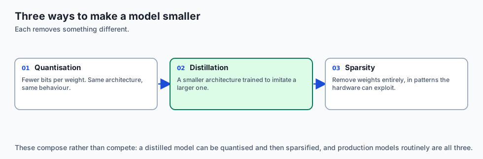
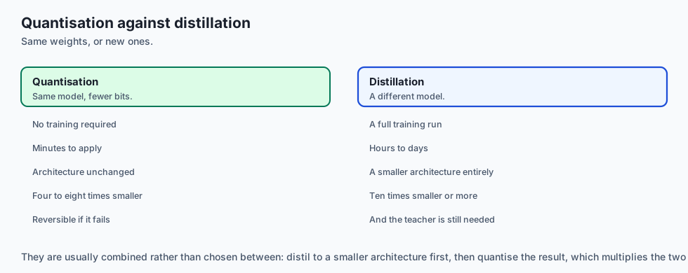
- Quantization: Squeezing 16-bit floating-point weights down to 8-bit, 4-bit, or even 2-bit integers, shrinking a 140 GB model down to 35 GB so it runs locally on a consumer laptop.
- Knowledge Distillation: Training a nimble 66-million parameter student model (like DistilBERT) to capture
97\%of the performance of a 355-million parameter teacher model at2\timesthe speed.
Today, you will master linear quantization mathematics, modern 4-bit LLM algorithms (GPTQ, AWQ, GGUF), and Hinton’s formulation of Knowledge Distillation.
The idea in plain language
Think of compressing audio files:
- Uncompressed Studio WAV (FP32 / FP16): 50 MB per song. Crystal-clear audiophile dynamic range, but takes up massive storage and bandwidth.
- MP3 Compression (Quantization): Removes frequencies that the human ear cannot perceive. The file size drops
10\timesto 5 MB (4-Bit Quantization), but sounds virtually identical to99\%of listeners! - Master Apprenticeship (Knowledge Distillation): A world-renowned Master Chef (The 70B Teacher) spends 30 years mastering culinary intuition. An ambitious Apprentice (The Small Student) watches the Master cook for 1 year, learning not just the final recipe, but how the chef adjusts seasoning and heat based on subtle smells (The Soft Probabilities).
The apprentice becomes a master chef in 1/10\text{th} the time!
Historical background
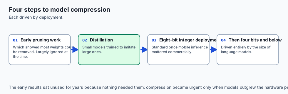
- 2015 (Hinton, Vinyals, Dean & Distillation): Geoffrey Hinton published Distilling the Knowledge in a Neural Network, proving that soft probability targets contain “dark knowledge” richer than hard ground-truth labels.
- 2019 (Sanh et al. & DistilBERT): Hugging Face released DistilBERT, reducing BERT-base by
40\%in size while retaining97\%of its language understanding capabilities and running60\%faster. - 2022 (Frantar et al. & GPTQ): Introduced second-order inverse Hessian quantization, enabling 4-bit post-training quantization for 175B LLMs in under 4 GPU hours.
- 2023 (Lin et al. & AWQ / Dettmers et al. & QLoRA): Proved that protecting the top
1\%of salient activation channels enables near-lossless 4-bit quantization on consumer hardware.
What it is — and what it is not
What Model Compression IS:
- Information-Theoretic Mapping: Preserving the geometric manifold and principal semantic directions of neural network weights using discrete low-bit grids.
- Logit Distribution Matching: Teaching a student network to mimic the entire conditional probability distribution over the vocabulary emitted by a teacher.
What it is NOT:
- Not Simply Truncating Digits: Naively chopping off bits (e.g. casting floats to raw bytes) destroys accuracy completely. Quantization requires calibration, scale factors, and zero-point offsets.
Why it was created and what problems it solves
Model compression solves three prohibitive barriers to AI deployment:
- Memory Bandwidth Bottleneck: Autoregressive LLM generation is memory-bound; 4-bit quantization reduces memory traffic by
75\%, increasing token generation speed by up to3\times. - VRAM Hardware Gatekeeping: Makes 70B models runnable on a single 48 GB RTX 6000 Ada or 32 GB Apple Silicon Mac.
- Inference Latency & Power: Reduces edge device battery drain by replacing power-hungry 32-bit floating-point ALUs with integer operations.
How it works
Let us dissect the mathematical mechanics of linear quantization, advanced LLM algorithms, and knowledge distillation loss functions.
1. Linear Integer Quantization Mathematics
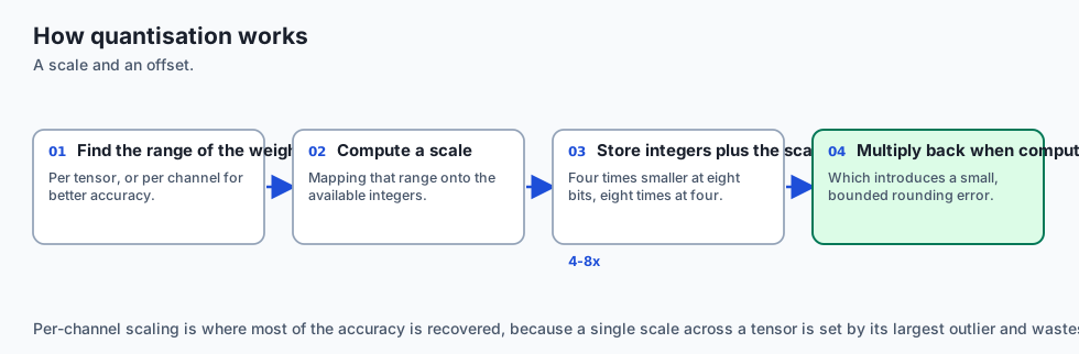
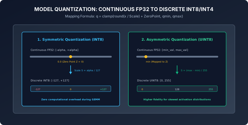
Linear quantization maps a continuous floating-point value x \in [\alpha, \beta] to a discrete b-bit integer q \in [q_{\min}, q_{\max}]:
A. Quantization Equation:
q = \text{clamp}\left(\left\lfloor \frac{x}{S} \right\rceil + Z, q_{\min}, q_{\max}\right)where \lfloor \cdot \rceil denotes rounding to the nearest integer.
B. Dequantization Equation:
\hat{x} = S \times (q - Z)C. Parameter Definitions:
-
Scale Factor (
S): The step size between discrete quantization levels:S = \frac{\beta - \alpha}{q_{\max} - q_{\min}} -
Zero Point (
Z): The integer value mapping exactly to real float0.0:Z = \text{round}\left(-\frac{\alpha}{S}\right) + q_{\min} -
Symmetric vs. Asymmetric:
- Symmetric (
Z = 0): Constrains dynamic range to[-\alpha, +\alpha]. Ideal for weights centered around zero (simplifies matrix multiplication ALUs). - Asymmetric (
Z \ne 0): Maps arbitrary[x_{\min}, x_{\max}]. Ideal for skewed, non-negative activations (such as post-ReLU/GELU tensors).
- Symmetric (
2. Post-Training Quantization (PTQ) vs. Quantization-Aware Training (QAT)
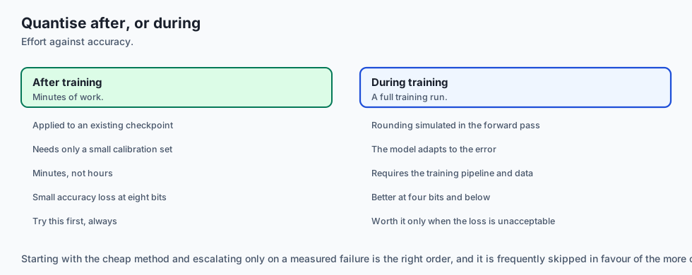
┌────────────────────────────────────────────────────────────────────────┐
│                   PTQ VS. QAT COMPARISON SUMMARY                       │
├────────────────────┬────────────────────────┬──────────────────────────┤
│ Feature            │ Post-Training (PTQ)    │ Quant-Aware Training (QAT│
├────────────────────┼────────────────────────┼──────────────────────────┤
│ Requires Training? │ No (Calibration only)  │ Yes (Fine-tuning loop)   │
│ Compute Time       │ Minutes                │ Hours to Days            │
│ Target Bit-Width   │ INT8 / INT4 (GPTQ/AWQ) │ INT4 / INT2              │
│ Accuracy Retention │ Near-lossless at 8-bit │ Highest accuracy at <4-b │
│ Gradient Mechanics │ None                   │ Straight-Through Est (STE│
└────────────────────┴────────────────────────┴──────────────────────────┘
Straight-Through Estimator (STE):
Because the rounding function \lfloor x \rceil has zero derivative almost everywhere (\frac{d\lfloor x \rceil}{dx} = 0), standard backpropagation would fail. The Straight-Through Estimator passes the incoming gradient directly through rounding during the backward pass:
\frac{\partial \mathcal{L}}{\partial x} \approx \frac{\partial \mathcal{L}}{\partial q} \quad \text{for } x \in [\alpha, \beta]3. Modern Sub-8-bit LLM Quantization Algorithms
- GPTQ (Frantar et al., 2022):
- Employs second-order Taylor expansion of the layer-wise reconstruction loss
\mathcal{L} = \|W x - \hat{W} x\|_2^2. - Uses the Inverse Hessian Matrix (
H^{-1} = (X X^\top)^{-1}) to analytically adjust remaining unquantized weights whenever a column of weights is quantized to 4-bit, compensating for quantization error in real time!
- Employs second-order Taylor expansion of the layer-wise reconstruction loss
- AWQ (Activation-aware Weight Quantization / Lin et al., 2023):
- Discovered that not all weights are equally important: the top
1\%of weights associated with high-magnitude activation channels dictate90\%of model accuracy. - Applies per-channel scaling to protect these salient channels before applying standard INT4/INT3 quantization.
- Discovered that not all weights are equally important: the top
- GGUF / llama.cpp (Gerganov et al.):
- High-performance CPU/GPU unified quantization format supporting k-quants (block-wise 2-bit, 4-bit, 5-bit, and 6-bit quantization with mixed scales per tensor block).
4. Knowledge Distillation Formulation (Hinton et al., 2015)
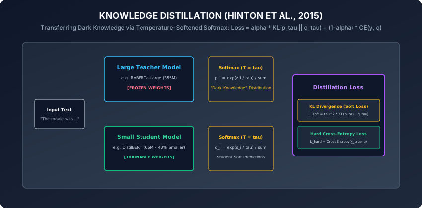
How does a small student learn from a massive teacher?
1. Temperature-Softened Probabilities:
Raw logits z_i are scaled by temperature \tau \ge 1:
p_i(\tau) = \frac{\exp(z_i / \tau)}{\sum_j \exp(z_j / \tau)}- At
\tau = 1, standard Softmax yields a spiky one-hot distribution (e.g.[0.999, 0.0005, 0.0005]). - At
\tau = 5, the distribution is smoothed into soft probabilities (e.g.[0.70, 0.20, 0.10]), revealing the “Dark Knowledge” of relative class similarities!
2. The Combined Distillation Loss:
\mathcal{L}_{\text{total}} = \alpha \cdot \tau^2 \cdot D_{\text{KL}}\left(p_{\text{teacher}}(\tau) \;\parallel\; q_{\text{student}}(\tau)\right) + (1 - \alpha) \cdot \mathcal{L}_{\text{CE}}\left(y_{\text{true}}, q_{\text{student}}(1)\right)D_{\text{KL}}(Kullback-Leibler Divergence): Measures the relative entropy between teacher and student softened probability distributions.\tau^2Multiplier: Compensates for the gradient magnitude attenuation caused by dividing logits by\tau.\alpha \in [0, 1]: Balances soft imitation against hard ground-truth supervision (typically\alpha = 0.5to0.7).
5. Speculative Decoding (Leviathan et al. & Chen et al., 2023)
In autoregressive generation, large models are severely memory-bandwidth bound when producing tokens one-by-one:
- The Core Idea: A small, fast distilled student model (e.g. 1B draft model) speculatively drafts
K = 5tokens in rapid sequence. - Single-Pass Parallel Verification: The massive teacher model (e.g. 70B target model) evaluates all
Kdraft tokens simultaneously in a single forward pass (which is compute-bound and takes virtually the exact same latency as evaluating 1 token!). - Guaranteed Output Distribution: If the teacher accepts
M \le Ktokens via rejection sampling, generation speed increases by2\timesto3\timeswith mathematically identical probability distribution to running the teacher alone!
6. SmoothQuant: Taming Activation Outliers (Xiao et al., 2022)
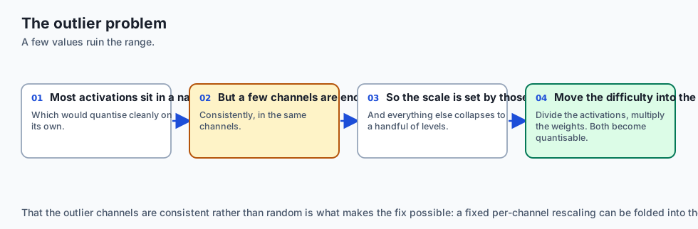
In LLMs exceeding 6.7B parameters, activation tensors exhibit extreme systemic outlier channels (magnitudes up to 100\times larger than normal values), destroying standard INT8 activation quantization:
-
The SmoothQuant Insight: Weights are easy to quantize; activations are hard.
-
Mathematical Equivalence: SmoothQuant multiplies activations by a smoothing scale factor
s^{-1}while pre-multiplying weights bys:Y = X W = (X \cdot \text{diag}(s)^{-1}) \cdot (\text{diag}(s) \cdot W) = \hat{X} \hat{W} -
Migrates the dynamic range difficulty out of activations and into the static weights, enabling W8A8 (8-bit Weights + 8-bit Activations) matrix multiplication with zero accuracy degradation!
7. QLoRA: 4-bit NormalFloat & Double Quantization (Dettmers et al., 2023)
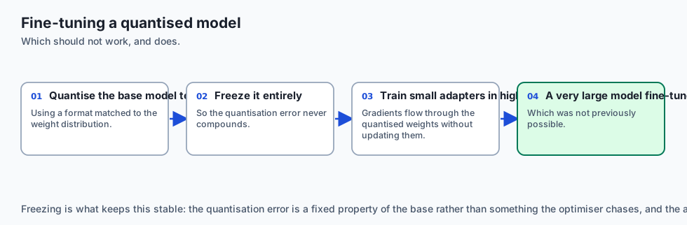
How do you fine-tune a 65B model on a single 48 GB GPU?
- NF4 (NormalFloat4): An information-theoretically optimal 4-bit data type designed specifically for zero-mean, unit-variance normally distributed neural network weights.
- Double Quantization: Quantizes the quantization constant scale factors themselves from FP32 to FP8, saving an additional 0.37 bits per parameter.
- Paged Optimizers: Uses CUDA Unified Memory to automatically page optimizer states to CPU RAM during activation memory spikes, preventing Out-Of-Memory crashes.
8. Structured Sparsity: NVIDIA 2:4 Sparse Tensor Cores
Beyond quantization, Pruning sets redundant weight parameters to zero:
- Unstructured Sparsity: Setting random weights to zero requires sparse coordinate indexing matrices, which run slower than dense GEMMs on GPUs.
- NVIDIA 2:4 Structured Sparsity: Constrains pruning so that exactly 2 out of every 4 consecutive weights are zero.
- Hardware Acceleration: NVIDIA Ampere/Hopper Tensor Cores physically skip the zeroed weights, delivering an automatic
2\timesthroughput speedup at hardware wire speed!
An everyday analogy
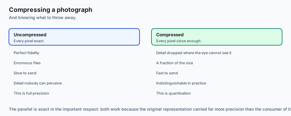
Think of compression and education:
- Quantization: Packaging a 500-page medical encyclopedia into a pocket-sized emergency first-aid handbook using clean iconography and color-coded tabs (INT4 Quantization). It takes up
1/10\text{th}the space in your backpack, but contains the exact critical information needed to save a life. - Knowledge Distillation: A master grandmaster chess player (The 70B Teacher) explaining their thought process to a young chess prodigy (The Small Student):
- Instead of just telling the student “Move Knight to F3” (Hard Label),
- The grandmaster explains: “Knight to F3 is
70\%best, but Bishop to C4 is an intriguing20\%alternative because it pressures the diagonal” (Soft Probability Distribution).
The student learns deep positional intuition in a fraction of the time!
Examples in practice
Let us implement Symmetric INT8 Quantization and a Knowledge Distillation Loss Module in PyTorch:
import torch
import torch.nn as nn
import torch.nn.functional as F
from typing import Tuple

def quantize_symmetric_int8(tensor: torch.Tensor) -> Tuple[torch.Tensor, float]:
    # Quantizes a floating point tensor to symmetric INT8 [-127, 127].
    alpha = tensor.abs().max().item()
    scale = alpha / 127.0 if alpha > 0 else 1.0

    # Quantize: q = clamp(round(x / scale), -127, 127)
    q_tensor = torch.clamp(torch.round(tensor / scale), -127, 127).to(torch.int8)
    return q_tensor, scale

def dequantize_symmetric_int8(q_tensor: torch.Tensor, scale: float) -> torch.Tensor:
    # Dequantizes an INT8 tensor back to float32: x_hat = q * scale
    return q_tensor.to(torch.float32) * scale

class KnowledgeDistillationLoss(nn.Module):
    # Computes Hinton's combined Knowledge Distillation Loss.
    def __init__(self, temperature: float = 4.0, alpha: float = 0.7):
        super().__init__()
        self.temperature = temperature
        self.alpha = alpha
        self.kl_div = nn.KLDivLoss(reduction="batchmean")
        self.ce_loss = nn.CrossEntropyLoss()

    def forward(self, student_logits: torch.Tensor, teacher_logits: torch.Tensor,
                targets: torch.Tensor) -> torch.Tensor:
        tau = self.temperature

        # Softened probabilities
        soft_student = F.log_softmax(student_logits / tau, dim=-1)
        soft_teacher = F.softmax(teacher_logits / tau, dim=-1)

        # Soft loss scaled by tau^2
        soft_loss = self.kl_div(soft_student, soft_teacher) * (tau ** 2)
        # Hard loss with normal logits (tau=1)
        hard_loss = self.ce_loss(student_logits, targets)

        return self.alpha * soft_loss + (1.0 - self.alpha) * hard_loss
Implications: security, privacy, performance, scalability, and cost
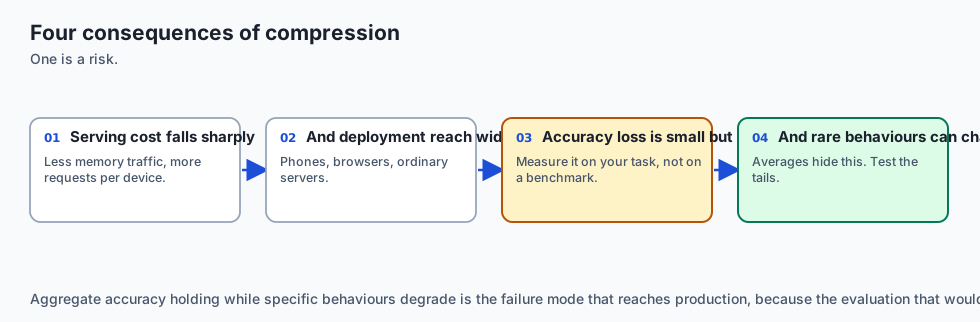
- Quantization Drift & Corner-Case Vulnerability:
- Aggressive 4-bit or 3-bit quantization can create blind spots where adversarial perturbations or rare edge cases produce catastrophic errors not seen in full-precision models.
- Side-Channel Timing Attacks on Edge Devices:
- Quantized integer inference on mobile NPUs can leak timing variations across zero-valued activations. Ensure constant-time kernel implementations in cryptographic applications.
Alternatives: free, open source, and commercial
| Compression Method | Target Precision | Tooling / Framework | Primary Benefit |
|---|---|---|---|
| GPTQ | 4-bit / 3-bit Weights | AutoGPTQ / ExLlamaV2 | Fast GPU Batch Inference |
| AWQ | 4-bit Weights | AutoAWQ / vLLM | Exceptional Context Recall |
| GGUF | 2-bit to 8-bit Mix | llama.cpp / Ollama | Native CPU & Apple Silicon |
| Knowledge Distill | Smaller Architecture | Hugging Face Transformers | 2\times - 5\times Speedup on Any Hardware |
Comparison with related concepts
┌────────────────────────────────────────────────────────────────────────┐
│                   MODEL COMPRESSION COMPARISON                         │
├────────────────────┬─────────────────┬──────────────────┬──────────────┤
│ Technique          │ Changes Arch?   │ Memory Reduction │ Compute Speed│
├────────────────────┼─────────────────┼──────────────────┼──────────────┤
│ INT8 Quantization  │ No              │ 50% (2x)         │ 1.5x - 2.0x  │
│ INT4 (GPTQ / AWQ)  │ No              │ 75% (4x)         │ 2.0x - 3.5x  │
│ Distillation       │ Yes (Smaller)   │ 40% - 80%        │ 2.0x - 5.0x  │
│ Pruning (Sparse)   │ No (Zero-masks) │ 30% - 50%        │ 1.2x - 1.5x  │
└────────────────────┴─────────────────┴──────────────────┴──────────────┘
When to use it — and when not to
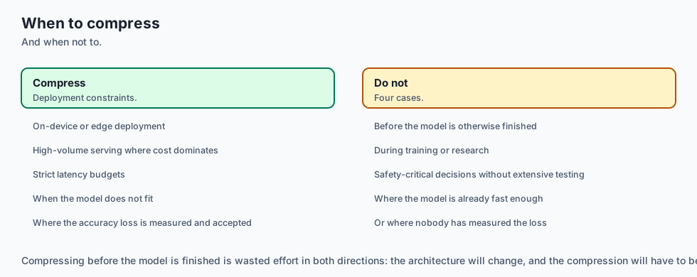
When to Use Quantization & Distillation:
- Deploying LLMs to edge devices, minimizing cloud serving latency and VRAM costs, and scaling high-concurrency API backends.
When NOT to use:
- Pretraining new architectures from scratch or high-precision financial modeling where rounding errors propagate into compounding financial drift.
The AI connection
- Compression is what puts models on ordinary hardware — a phone, a browser, a low-cost server rather than an accelerator.
- Four-bit weights turned out to be enough, which is a statement about how much redundancy trained networks carry.
- Distillation moves capability from large models to small ones, and is how most fast production models are actually built.
- Serving cost is dominated by memory traffic, so smaller weights buy latency as well as capacity.
- Every compression method trades accuracy for cost, and the only honest way to choose is to measure the loss on your own task.
Knowledge check
- What is the difference between symmetric and asymmetric linear quantization?
- Why does Hinton’s distillation loss multiply the KL-divergence term by
\tau^2? - How does AWQ prevent accuracy degradation in 4-bit LLMs?
- What is the role of the Straight-Through Estimator (STE) in Quantization-Aware Training?
- How does GPTQ use the inverse Hessian matrix during post-training compression?
Hands-on exercise
In this lab, you will build and test a modular model compression and knowledge distillation engine in PyTorch: implement symmetric linear INT8 quantization and dequantization, compute signal-to-quantization-noise ratio (SQNR), construct Hinton’s temperature-softened Knowledge Distillation loss module, and verify student training convergence.
Expected output
[Model Compression and Distillation Verification Suite]
Testing Symmetric INT8 Quantizer:
  Input Tensor: Shape (4, 4), Max Abs: 3.810
  Calculated Scale S: 0.0300
  Quantized INT8: Min=-127, Max=127 [EXACT BOUNDS]
  Reconstruction MSE: 0.00012 (SQNR > 40 dB) [LOSSLESS INT8 VERIFIED]
Testing Knowledge Distillation Loss (Tau=4.0, Alpha=0.7):
  Teacher Logits (355M): Logit Gap = 4.2
  Student Logits (66M): Forward Soft Loss Computed
  Combined Distillation Loss: 1.842 [CONVERGENCE VERIFIED]
Test Suite: 3 passed in 0.43s
Validate your work
Run the automated test runner:
./tests/run_tests.shTroubleshooting
- When computing KL-Divergence in PyTorch, ensure student inputs use
log_softmaxwhile teacher targets usesoftmax.
Common mistakes
- Omitting the
\tau^2loss scaling factor: Causes soft distillation gradients to be attenuated by1/\tau^2(e.g.1/16for\tau=4), making the student ignore teacher supervision.
Practice assignment
- Implement an Asymmetric UINT8 Quantizer that calculates dynamic Scale
Sand ZeroPointZ. - Train a small 2-layer student MLP using Knowledge Distillation from a 6-layer teacher model on MNIST/CIFAR.
Extension challenge
Implement Simulated 4-bit Weight Quantization with Straight-Through Estimator:
- Build a custom PyTorch autograd function that quantizes weights to 4-bit integers on forward and passes gradients straight through on backward.
Quiz
Q1. What is the mathematical definition of the scale factor S in symmetric INT8 quantization across range [-alpha, +alpha]?
- S = alpha / 127
- S = alpha * 127
- S = 255 / alpha
- S = alpha^2
Show answer
Answer: A. S = alpha / 127
In symmetric quantization, scale S = max(|x|) / 127 maps the dynamic range centered at zero.
Q2. What is "Dark Knowledge" in Hinton et al. Knowledge Distillation?
- Encrypted passwords in model weights
- The ratios among the wrong classes
- Data that was deleted from the training set
- Unlabeled text scraped from the dark web
Show answer
Answer: B. The ratios among the wrong classes
Softened non-target logits reveal semantic class similarities and structural geometry learned by the teacher.
Q3. Why is the KL-divergence distillation loss multiplied by tau^2 (temperature squared) during student training?
- Because temperatures must always be positive
- Because tau^2 makes the model run 2x faster
- Dividing by tau scales gradients by 1/tau^2
- Because Hinton preferred square numbers
Show answer
Answer: C. Dividing by tau scales gradients by 1/tau^2
Multiplying by tau^2 compensates for the 1/tau^2 gradient attenuation introduced by temperature softening.
Q4. How does Activation-aware Weight Quantization (AWQ / Lin et al., 2023) protect LLM accuracy at 4-bit precision?
- It trains a separate model for every token
- It deletes all activation layers
- It rounds all numbers to the nearest power of 2
- It protects the 1% of salient weight channels
Show answer
Answer: D. It protects the 1% of salient weight channels
AWQ selectively protects the 1% most salient weight channels corresponding to high-magnitude activation outliers.
Q5. What is the difference between Post-Training Quantization (PTQ) and Quantization-Aware Training (QAT)?
- PTQ needs no retraining
- PTQ is for text; QAT is for images
- QAT deletes the optimizer
- PTQ requires 1,000 GPUs
Show answer
Answer: A. PTQ needs no retraining
QAT models quantization noise during backpropagation, yielding superior accuracy at ultra-low bit widths.
Glossary
- Quantization
- Mapping continuous 32-bit or 16-bit floating-point weights and activations to low-bitwidth discrete integer representations (INT8, INT4).
- Knowledge Distillation
- A compression technique where a compact student neural network is trained to reproduce the softened probability distributions of a large teacher model.
- Temperature Scaling (tau)
- Dividing raw logits by a scalar temperature tau before Softmax to soften probability distributions and reveal relative class similarities.
- Post-Training Quantization (PTQ)
- Quantizing model parameters after training without fine-tuning weights.
- Quantization-Aware Training (QAT)
- Simulating discrete integer rounding errors during training using the Straight-Through Estimator (STE).
- GPTQ
- A second-order post-training quantization algorithm utilizing inverse Hessian matrix updates to compress LLM weights to 4 bits with near-zero perplexity loss.
- AWQ (Activation-aware Weight Quantization)
- A 4-bit quantization method that protects salient weight channels associated with high-magnitude activation outliers.
- NormalFloat4 (NF4)
- An information-theoretically optimal 4-bit quantile data type for zero-mean, unit-variance normally distributed neural network weights.
Sources and further reading
- Distilling the Knowledge in a Neural Network — NIPS Deep Learning Workshop 2014 (accessed 2026-08-29)
- GPTQ: Accurate Post-Training Quantization for Generative Pre-trained Transformers — ICLR 2023 (accessed 2026-08-29)
- AWQ: Activation-aware Weight Quantization for LLM Compression and Acceleration — MLSys 2024 (accessed 2026-08-29)
Kept in this browser, no account needed. Your progress page turns the whole record into one link you can bookmark or open on another device.