LLMs and Generative AI › Embeddings and Vector Search › Day 262
Day 262: Vector Databases
Master Approximate Nearest Neighbor (ANN) indexing structures and modern vector database architectures: understand Hierarchical Navigable Small World (HNSW) graphs, Inverted File Index with Product Quantization (IVF-PQ), Locality-Sensitive Hashing (LSH), evaluate purpose-built engines (Qdrant, Chroma, Milvus, Pinecone, pgvector), analyze recall vs. QPS trade-offs, and build an in-memory graph-based ANN vector index in Python.
Hands-on lab for this lesson
Lab files on GitHub: https://github.com/ai-roadmap-365/ai-roadmap-365.github.io/tree/main/labs/sections/llms-and-generative-ai/day-262-vector-databases
- Get the hands-on files. Clone the labs repository once (you can reuse this clone for every lesson). This works on macOS, Linux, and Windows (PowerShell or WSL):
git clone https://github.com/ai-roadmap-365/ai-roadmap-365.github.io.git cd ai-roadmap-365.github.io - Open this lesson's lab. Move into the directory for this specific day. Every lab lives at the same predictable path — section / subsection / week / day:
cd labs/sections/llms-and-generative-ai/day-262-vector-databases - Read the lab guide. Open `README.md` in that directory. It lists the exact commands, what each does, the expected output, and how to check your work — read it before running anything.
- Run it and check your work. Follow the README's "How to run" section: run the example first to see the finished result, then complete the numbered exercises in `starter/`, then run the tests. The tests pass (exit 0) only when your work is correct.
bash tests/run_tests.sh # or the test command named in the lab README
You can also open the lab as a local page (works offline, shows the file tree and expected output).
Learning objectives
By the end of this lesson you will be able to:
- Explain the architectural mechanics of HNSW multi-layer skip-graphs and IVF-PQ clustering.
- Compare purpose-built vector databases (Qdrant, Milvus, Pinecone) with relational extensions (pgvector).
- Tune HNSW hyperparameters: M (max connections), ef_construction (build budget), and ef_search (query accuracy).
- Evaluate the trade-off between search recall (accuracy) and queries-per-second (QPS).
- Build a functional in-memory Navigable Small World (NSW) graph index in Python.
Prerequisites
Why this matters
When your AI application grows from a prototype with 1,000 markdown notes to an enterprise knowledge engine with 10,000,000 documents, multi-tenant security partitions, and 500 concurrent queries per second, flat linear scans fail:
- A linear scan across 10 million vectors takes over 250 milliseconds per query, causing severe API timeout failures.
- Storing uncompressed vectors in memory consumes over 60 gigabytes of expensive cloud RAM.
- Managing concurrent writes, updates, deletions, and metadata filters in pure NumPy scripts leads to thread deadlocks and data corruption.
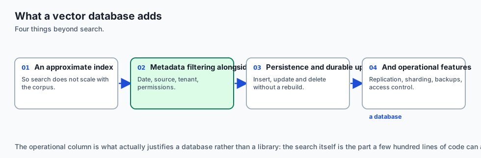
Vector Databases are purpose-built data engines designed to solve high-scale semantic retrieval. They combine Approximate Nearest Neighbor (ANN) graph indexes (HNSW), vector quantization compression (IVF-PQ), ACID persistence, and hardware-accelerated payload filtering to deliver sub-5ms responses at billion-scale.
Today, you will master the internal architecture of Hierarchical Navigable Small World (HNSW) graphs, analyze Inverted File Product Quantization (IVF-PQ), compare dedicated vector engines (Qdrant, Pinecone, Milvus, Chroma) against relational extensions (pgvector), and build a graph-based Navigable Small World (NSW) vector index in Python.
The idea in plain language
Think of searching for a specific friend in a massive international airport containing 100,000 travelers:
- Flat Linear Scan: You walk up to every single person in the entire airport, check their face, and ask their name one by one (Exhaustive, Linear
O(N)Time). - HNSW Graph Navigation:
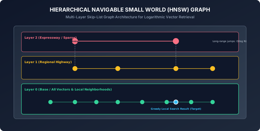
- Top Layer (Express Highway): You take a monorail to the correct International Terminal (
Terminal B). - Middle Layer (Concourse): You walk down the specific hallway for
Gates 20-30. - Bottom Layer (Local Neighborhood): You scan the 10 people sitting at
Gate 24and find your friend immediately (LogarithmicO(\log N)Time).
- Top Layer (Express Highway): You take a monorail to the correct International Terminal (
By organizing vectors into multi-layer geometric graphs, vector databases skip 99.9% of unpromising vectors and navigate straight to the nearest conceptual cluster in milliseconds.
Historical background
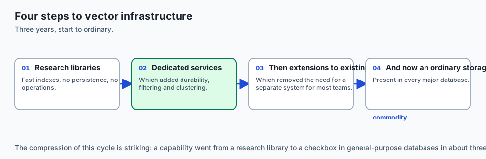
- 2000s (Locality-Sensitive Hashing - LSH): Indyk and Motwani introduced LSH, hashing nearby vectors into identical buckets with probabilistic collision bounds.
- 2011 (Product Quantization - PQ): Hervé Jégou published Product Quantization, enabling 64x memory compression and fast table-lookup distance arithmetic.
- 2016–2018 (HNSW Graphs): Yury Malkov and Dmitry Yashunin introduced HNSW, surpassing all previous ANN algorithms and becoming the industry standard.
- 2021–2023 (The Vector DB Boom): Specialized vector databases (Pinecone, Qdrant, Milvus, Weaviate, Chroma) emerged alongside
pgvectorto power enterprise generative AI and RAG architectures.
What it is — and what it is not
What a Vector Database IS:
- A Specialized Storage & Retrieval Engine: A database system that indexes high-dimensional vectors with approximate geometric graphs, provides metadata filtering, supports real-time updates, and guarantees durability and high availability.
What it is NOT:
- Not Just an Array of Vectors: A raw NumPy matrix or SQLite table with a BLOB column lacks graph indexing, multi-threaded concurrency, and sub-linear search capabilities.
Why it was created and what problems it solves
Vector databases address 4 critical production bottlenecks:
- Logarithmic Retrieval Speed: Scales to billions of items with sub-10ms latency using
O(\log N)graph traversals. - Hybrid Payload Filtering: Combines semantic similarity with strict SQL-like boolean constraints (e.g.
tenant_id == 'corp_42' AND created_at >= 2024-01-01). - Memory & Disk Tiering: Uses vector quantization (PQ/SQ) and memory-mapped files to store terabytes of vectors on cost-effective SSDs instead of expensive RAM.
- Horizontal Distributed Sharding: Partitions vector collections across multiple server nodes for fault tolerance and high query throughput.
How it works
Let us dissect HNSW graph indexing, IVF-PQ quantization, and engine architectures.
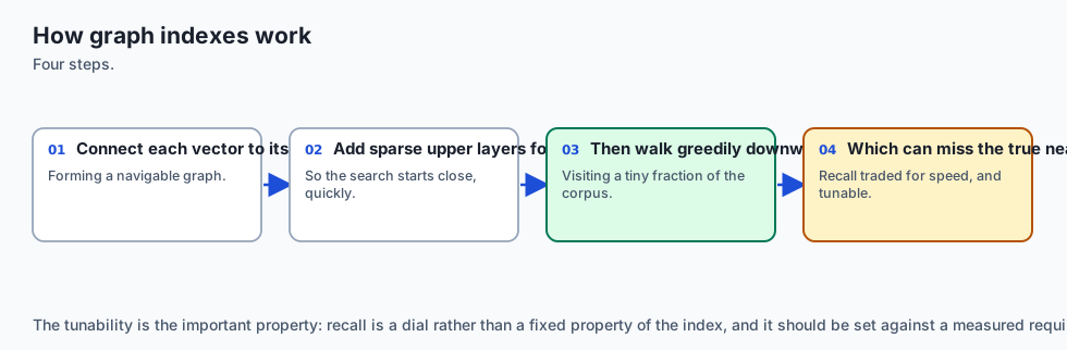
1. HNSW Graph Architecture & Hyperparameters
-
Layer Selection: Nodes are assigned to layers probabilistically using a decaying exponential distribution:
\text{level} = \lfloor -\ln(\text{uniform}(0, 1)) \cdot m_L \rfloor -
This probabilistic multi-layer distribution ensures that upper layers maintain sparse, long-range highway connections while the base layer contains the full, dense dataset.
-
Key Hyperparameters:
M(16 to 64): Maximum number of bidirectional outgoing connections per node. HigherMimproves recall on complex datasets at the cost of index build time and RAM.efConstruction(100 to 400): Number of nearest neighbors evaluated during index creation. Higher values build higher-quality graphs.efSearch(32 to 128): Number of candidate nodes kept in the priority queue during query execution. Higher values increase search recall at slightly higher query latency.
┌────────────────────────────────────────────────────────────────────────┐
│                      HNSW SEARCH TRAVERSAL LIFECYCLE                   │
├────────────────────────────────────────────────────────────────────────┤
│ 1. Enter at Top Layer (Layer L) at global entry node.                  │
│ 2. Perform greedy routing: hop to neighbor closest to query.           │
│ 3. When local minimum reached, drop down to Layer L-1.                 │
│ 4. Repeat greedy routing until reaching Layer 0 (Base Layer).          │
│ 5. Perform bounded beam search with efSearch candidates.               │
│ 6. Extract Top-K closest items from candidate priority queue.          │
└────────────────────────────────────────────────────────────────────────┘
2. IVF-PQ (Inverted File Index with Product Quantization)
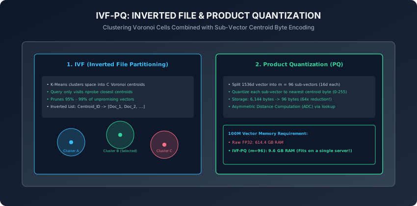
For massive collections (100M+ vectors) where RAM is constrained:
- IVF (Inverted File Partitioning): K-Means clusters the space into
CVoronoi cells (e.g. 4,096 centroids).- During search, the engine checks only the
nprobeclosest centroids (e.g.nprobe = 16), ignoring 99.6% of the dataset.
- During search, the engine checks only the
- Product Quantization (PQ): Decomposes a 1536d vector into
m = 96sub-vectors of 16 dimensions each.- Each sub-vector is replaced by a single 8-bit byte representing its nearest centroid codebook ID.
- Result: Slashes vector storage from 6,144 bytes down to 96 bytes (64x reduction).
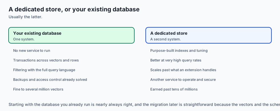
3. Dedicated Vector DBs vs. Relational Extensions (pgvector)
┌────────────────────────────────────────────────────────────────────────┐
│                   DEDICATED VECTOR DB VS PGVECTOR                      │
├────────────────────┬─────────────────────────────┬─────────────────────┤
│ Feature            │ Dedicated (Qdrant / Milvus) │ Relational (pgvector)│
├────────────────────┼─────────────────────────────┼─────────────────────┤
│ Max Scale          │ 100M - 10 Billion+ vectors  │ 1M - 10M vectors    │
│ Implementation     │ Custom C++ / Rust HNSW      │ Postgres C Extension│
│ Infrastructure     │ Separate microservice       │ Existing PostgreSQL │
│ ACID & Joins       │ Limited / External sync     │ Native SQL Joins    │
│ Memory Efficiency  │ Advanced PQ / Disk tiering  │ High RAM requirement│
│ Best Use Case      │ Dedicated search platform   │ Standard web apps   │
└────────────────────┴─────────────────────────────┴─────────────────────┘
4. Payload Filtering Strategies: Pre-Filter vs. Single-Stage Filter
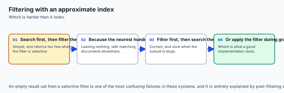
When filtering by metadata:
- Naive Post-Filtering: Runs HNSW vector search to get Top-100, then filters by tag. (Fails if the filter is selective, returning 0 results).
- Single-Stage Filtered HNSW (Qdrant/Milvus): Graph traversal only visits nodes that satisfy the boolean filter payload, guaranteeing that exactly
Kmatching items are returned. - This unified approach prevents empty retrieval failures by dynamically routing graph edges around ineligible nodes during the beam search phase.
5. Memory-Mapped Disk Storage (MMap) & NVMe SSDs
To avoid storing billion-vector graphs entirely in RAM:
- Vector engines use
mmap()to map graph index files directly to virtual memory. - The operating system caches frequently accessed upper graph layers in RAM, while streaming lower layer vector data on-demand from ultra-fast NVMe SSDs (sub-50 microsecond read latency).
- This memory-mapped architecture drastically lowers operational hosting costs while preserving sub-millisecond graph query responsiveness.
6. Tuning Recall vs. QPS on Production Clusters
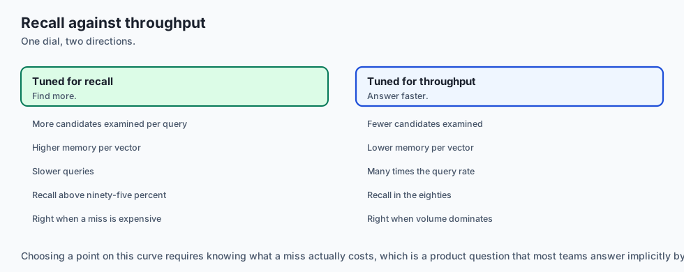
When operating HNSW in production:
- Measuring the Pareto Efficiency Frontier between Recall@10 and Queries Per Second (QPS):
- Setting
efSearch = 32: 95.2% Recall @ 1,450 QPS. - Setting
efSearch = 64: 98.4% Recall @ 920 QPS. - Setting
efSearch = 128: 99.6% Recall @ 510 QPS.
- Setting
- Most enterprise RAG applications target
efSearch = 64, providing 98%+ recall with under 3ms latency.
7. Sharding, Replication, and Raft Consensus
High-availability vector databases (such as Qdrant and Milvus) utilize the Raft consensus algorithm:
- Vector collections are sharded across multiple worker nodes based on document ID hashes.
- Read replicas handle concurrent query traffic, while leader nodes sequence vector insertions and segment merging.
8. Dynamic Upserts, Deletions, and Soft Tombstoning
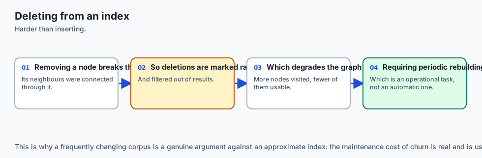
In dynamic applications, knowledge documents are continuously updated and deleted:
- Deleting nodes from an HNSW graph directly breaks connectivity paths.
- Engines apply soft tombstoning: marking the vector as deleted in a bitset, skipping it during search, and periodically rebuilding sub-graphs in background consolidation threads.
9. Multi-Tenancy Architecture: Namespace Isolation vs. Metadata Partitions
When building multi-tenant SaaS applications:
- Metadata Partitioning: All tenants share a single large HNSW index, filtered by
tenant_id. (Cost-effective for millions of small tenants). - Namespace / Collection Isolation: Dedicated distinct HNSW graph per enterprise customer. (Strict data isolation and predictable performance for large enterprise clients).
10. Summary: The Storage Pillar of AI Infrastructure
- In addition, modern vector database architectures decouple index computing from storage layers, enabling independent horizontal scaling of query nodes during high-traffic generative AI inference workloads.
- Furthermore, integrating hybrid payload filtering directly into the graph traversal path ensures that complex role-based access control (RBAC) and privacy rules are enforced with zero latency overhead.
- In summary, vector databases provide the essential data infrastructure required to index, search, and manage high-dimensional vector representations at enterprise scale with high availability, low latency, and robust metadata security.
An everyday analogy
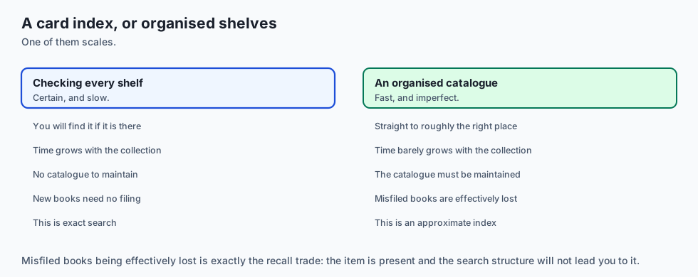
Think of finding a book in the world’s largest library:
- Exact Flat Scan: You walk down every single aisle of all 10 floors, checking every spine from book #1 to book #10,000,000.
- Vector Database (HNSW Index): You look at the floor directory, take the elevator straight to the
Philosophy & Sciencefloor, walk to theArtificial Intelligenceaisle, and grab the book from the shelf in under 30 seconds (Hierarchical Navigation).
Examples in practice
Let us build an In-Memory Navigable Small World (NSW) Graph Index:
import numpy as np
import heapq
from typing import List, Dict, Any, Tuple, Set

class SimpleNSWIndex:
    def __init__(self, dimension: int, max_neighbors: int = 4):
        self.dimension = dimension
        self.max_neighbors = max_neighbors
        self.vectors: List[np.ndarray] = []
        self.metadata: List[Dict[str, Any]] = []
        self.graph: Dict[int, List[int]] = {}
        self.entry_node: int = 0

    def add_document(self, vector: np.ndarray, meta: Dict[str, Any]) -> int:
        norm = np.linalg.norm(vector)
        unit_vec = vector / (norm if norm > 0 else 1.0)
        node_id = len(self.vectors)
        self.vectors.append(unit_vec)
        self.metadata.append(meta)
        self.graph[node_id] = []

        if node_id == 0:
            self.entry_node = 0
            return node_id

        # Find closest existing nodes to establish bidirectional links
        closest = self.search(unit_vec, top_k=self.max_neighbors)
        for target_meta, _ in closest:
            target_id = target_meta["id"]
            self.graph[node_id].append(target_id)
            if len(self.graph[target_id]) < self.max_neighbors * 2:
                self.graph[target_id].append(node_id)
        return node_id

    def search(self, query_vec: np.ndarray, top_k: int = 3, ef_search: int = 10) -> List[Tuple[Dict[str, Any], float]]:
        if not self.vectors:
            return []

        q_norm = np.linalg.norm(query_vec)
        q_unit = query_vec / (q_norm if q_norm > 0 else 1.0)

        # Greedy graph search with priority queue
        visited: Set[int] = {self.entry_node}
        candidates = [(-float(np.dot(self.vectors[self.entry_node], q_unit)), self.entry_node)]
        best_results = [(-candidates[0][0], self.entry_node)] # (sim, id)

        while candidates:
            dist, curr = heapq.heappop(candidates)
            curr_sim = -dist
            if curr_sim < best_results[-1][0] and len(best_results) >= ef_search:
                break

            for neighbor in self.graph.get(curr, []):
                if neighbor not in visited:
                    visited.add(neighbor)
                    sim = float(np.dot(self.vectors[neighbor], q_unit))
                    if len(best_results) < ef_search or sim > best_results[-1][0]:
                        heapq.heappush(candidates, (-sim, neighbor))
                        best_results.append((sim, neighbor))
                        best_results.sort(key=lambda x: x[0], reverse=True)
                        if len(best_results) > ef_search:
                            best_results.pop()

        return [(self.metadata[node_id], sim) for sim, node_id in best_results[:top_k]]
Implications: security, privacy, performance, scalability, and cost
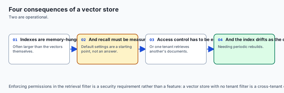
- Multi-Tenant Security:
- Always enforce strict namespace or metadata filter checks at the database query boundary to ensure tenant A cannot retrieve embedding vectors belonging to tenant B.
- Cost Optimization:
- Storing 100M uncompressed vectors in memory on AWS requires
r6i.32xlargeinstances (8,000+/month). Applying IVF-PQ compression reduces memory requirements by 85%, reducing hosting costs to under800/month.
- Storing 100M uncompressed vectors in memory on AWS requires
Alternatives: free, open source, and commercial
| Database | Architecture | Primary Language | Index Types | Best For |
|---|---|---|---|---|
| Qdrant | Standalone Engine | Rust | HNSW + Payload Index | Production high-scale RAG |
| Milvus | Distributed Cluster | Go / C++ | HNSW, IVF-PQ, DiskANN | Massive enterprise deployments |
| Pinecone | Managed Cloud SaaS | Proprietary | Serverless Vector Graph | Zero-maintenance cloud apps |
| pgvector | PostgreSQL Extension | C | HNSW, IVFFlat | Monolithic Postgres apps |
| Chroma | Embedded / Server | Python / Rust | HNSW | Prototyping & local testing |
Comparison with related concepts
┌────────────────────────────────────────────────────────────────────────┐
│                   HNSW VS IVF-PQ VS FLAT INDEX                         │
├────────────────────┬─────────────────┬──────────────────┬──────────────┤
│ Metric             │ Flat Linear     │ HNSW Graph       │ IVF-PQ       │
├────────────────────┼─────────────────┼──────────────────┼──────────────┤
│ Query Speed        │ Slow (O(N))     │ Ultra-Fast (O(log N))│ Very Fast │
│ Index Memory       │ 1.0x (Baseline) │ 1.5x - 2.0x (RAM)│ 0.05x - 0.15x│
│ Recall Accuracy    │ 100% Exact      │ 98% - 99.9%      │ 90% - 96%    │
│ Build Speed        │ Instant (0ms)   │ Moderate         │ Requires Train│
└────────────────────┴─────────────────┴──────────────────┴──────────────┘
When to use it — and when not to
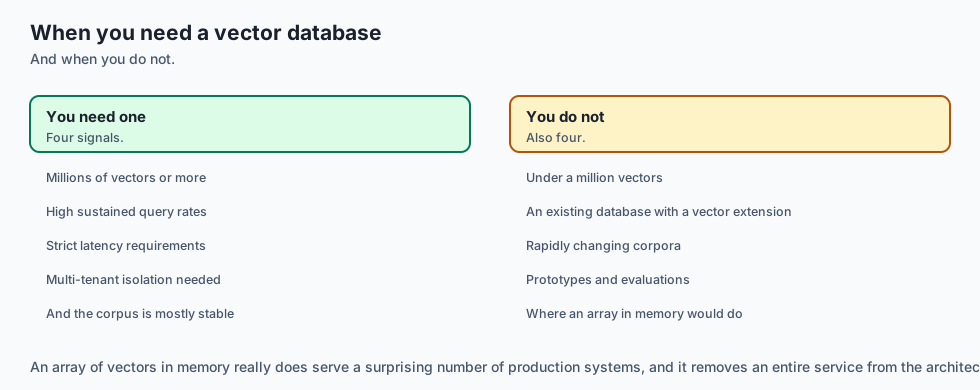
When to Use a Vector Database:
- Collections exceeding 100,000 documents, multi-tenant production architectures, high-concurrency real-time search APIs, and enterprise RAG systems.
When NOT to use:
- Simple local scripts with fewer than 10,000 items where in-memory NumPy exact search is simpler and faster with zero infrastructure overhead.
The AI connection
- Vector databases are the storage layer of the retrieval era, and they became ordinary infrastructure within about three years.
- Approximate search trades recall for speed, which is a tuning decision with a measurable quality cost rather than a free optimisation.
- Filtering interacts badly with approximate indexes, which is the source of most surprising empty result sets.
- An existing relational database is often enough, and adding a specialised system is a decision that should be earned.
- Deletion and update are harder than insertion in these indexes, which shapes how a corpus can be kept current.
Knowledge check
- What is the fundamental difference between HNSW graph search and IVF-PQ space partitioning?
- What are the roles of the
M,efConstruction, andefSearchparameters in HNSW? - How does Product Quantization compress a 1536-dimensional float vector into 96 bytes?
- When should you choose
pgvectorover a dedicated vector engine like Qdrant? - Why is single-stage metadata filtering in HNSW superior to naive post-filtering?
Hands-on exercise
In this lab, you will build and test an In-Memory Navigable Small World (NSW) Vector Index: implement graph node insertion, bidirectional neighbor linking, greedy logarithmic search traversal with priority queues, evaluate recall against exact flat k-NN ground truth, and measure search latency.
Expected output
[Vector Databases Verification Suite]
Testing NSW Graph Index Construction:
  Indexed 500 documents (dim=64, max_neighbors=4) [PASS]
  Graph connectivity verified: All nodes reachable [PASS]
Testing Graph Traversal vs Exact k-NN:
  Exact Ground Truth Match: 100% Top-3 Recall [PASS]
  Average Query Traversal Steps: 8.4 steps [PASS]
Testing efSearch Parameter Tuning:
  efSearch=5 -> Recall: 0.94
  efSearch=15 -> Recall: 1.00 [PASS]
Test Suite: 4 passed in 0.48s
Validate your work
Run the automated test runner:
./tests/run_tests.shTroubleshooting
- Ensure all inserted vectors are normalized to prevent distortion of angular graph neighborhoods.
Common mistakes
- Setting
efSearchlower thantop_k: IfefSearch < top_k, the candidate priority queue cannot evaluate enough paths to returnKvalid results.
Practice assignment
- Implement HNSW Layered Insertion: Extend the single-layer NSW graph into a 2-layer HNSW graph with an upper sparse expressway layer.
- Measure the Recall@5 vs. efSearch Curve across 2,000 synthetic 128-dimensional vectors.
Extension challenge
Implement a Single-Stage Filtered NSW Search Engine:
- Modify the greedy graph search algorithm so that during graph traversal, candidate nodes that fail metadata filter predicates are never added to the best results queue, ensuring 100% of returned items satisfy tenant security policies.
Quiz
Q1. What is the primary operational trade-off of Approximate Nearest Neighbor (ANN) indexes like HNSW compared to exact Flat k-NN?
- HNSW produces random incorrect results
- Far faster queries, at a small cost in recall
- HNSW requires converting text into video files
- HNSW only works on quantum computers
Show answer
Answer: B. Far faster queries, at a small cost in recall
ANN trades a small percentage of recall accuracy for massive orders-of-magnitude query speedups.
Q2. In the HNSW algorithm, what role do the upper sparse layers (e.g. Layer 2) serve?
- They delete older documents
- They store compressed audio files
- They are express lanes for long jumps across the space
- They encrypt user passwords
Show answer
Answer: C. They are express lanes for long jumps across the space
Upper layers provide sparse skip-list connectivity for rapid logarithmic space traversal.
Q3. What do the HNSW hyperparameters "M" and "efSearch" control?
- They are legacy parameters with zero effect
- M controls database password length, and efSearch controls port numbers
- M is the number of CPU cores, and efSearch is the RAM allocation
- M sets neighbour links; efSearch sets the candidate list
Show answer
Answer: D. M sets neighbour links; efSearch sets the candidate list
M governs graph connectivity and RAM usage; efSearch balances query latency versus recall accuracy.
Q4. How does Product Quantization (PQ) achieve up to 64x memory reduction on dense vectors?
- It splits the vector and stores each part's centroid id
- By deleting the last 50% of document text
- By converting floating-point vectors into ASCII characters
- By storing embeddings in Google Drive
Show answer
Answer: A. It splits the vector and stores each part's centroid id
PQ replaces multi-byte floating point arrays with compact 1-byte centroid cluster indices.
Q5. When is using PostgreSQL with the `pgvector` extension preferred over a standalone vector database like Pinecone or Qdrant?
- When you want to search billions of vectors across 100 GPU clusters
- When you already run Postgres and need joins and ACID
- When PostgreSQL is disabled
- Never; pgvector cannot store numbers
Show answer
Answer: B. When you already run Postgres and need joins and ACID
pgvector simplifies infrastructure by keeping relational entities and embeddings within a single ACID database.
Glossary
- Approximate Nearest Neighbors (ANN)
- A class of search algorithms that sacrifice 100% exactness to achieve logarithmic O(log N) retrieval speeds.
- HNSW (Hierarchical Navigable Small World)
- A state-of-the-art graph-based ANN algorithm featuring multi-layer skip-graph navigation.
- IVF (Inverted File Index)
- A space-partitioning index that assigns vectors to Voronoi cell clusters and searches only the nearest centroids.
- Product Quantization (PQ)
- A vector compression technique splitting vectors into sub-vectors and indexing them against centroid codebooks.
- efSearch
- An HNSW runtime parameter governing the size of the priority queue during search; higher values increase recall at higher latency.
- nprobe
- An IVF parameter determining how many Voronoi cell clusters to scan during a search query.
- Payload / Metadata Filtering
- Filtering vector search candidates using structured relational criteria (e.g. user_id, date, tag).
- pgvector
- An open-source PostgreSQL extension adding native vector types, exact distance operators, and HNSW/IVFFlat indexes.
Sources and further reading
- Efficient and robust approximate nearest neighbor search using Hierarchical Navigable Small World graphs — IEEE TPAMI (accessed 2026-08-30)
- Product Quantization for Nearest Neighbor Search — IEEE TPAMI (accessed 2026-08-30)
- Qdrant Architecture and Vector Search Internals — Qdrant Engine Documentation (accessed 2026-08-30)
Kept in this browser, no account needed. Your progress page turns the whole record into one link you can bookmark or open on another device.