Programming with Python › SQL and Relational Databases › Day 87
Day 87: Joins and Relationships
After this lesson you will be able to say why data belongs in more than one table — by reproducing the update, insertion and deletion anomalies of a single wide table yourself — and then put the pieces back together on demand: modelling one-to-many with the key on the many side and many-to-many with a junction table keyed on the pair, writing inner, left outer, cross, self and multi-table joins while being able to state exactly which rows each keeps and which columns it fills with NULL, reaching for the LEFT JOIN plus IS NULL idiom whenever a question is about absence, avoiding the two separate mistakes that turn a per-group count of zero into a wrong answer, knowing why an outer join predicate belongs in ON rather than WHERE, proving for yourself that SQLite enforces no foreign key until PRAGMA foreign_keys = ON is issued on that connection, and implementing both a nested-loop and a hash join in plain Python so that the algorithm the query planner is choosing between is one you have written.
Hands-on lab for this lesson
Lab files on GitHub: https://github.com/ai-roadmap-365/ai-roadmap-365.github.io/tree/main/labs/sections/programming-with-python/day-087-joins-and-relationships
- Get the hands-on files. Clone the labs repository once (you can reuse this clone for every lesson). This works on macOS, Linux, and Windows (PowerShell or WSL):
git clone https://github.com/ai-roadmap-365/ai-roadmap-365.github.io.git cd ai-roadmap-365.github.io - Open this lesson's lab. Move into the directory for this specific day. Every lab lives at the same predictable path — section / subsection / week / day:
cd labs/sections/programming-with-python/day-087-joins-and-relationships - Read the lab guide. Open `README.md` in that directory. It lists the exact commands, what each does, the expected output, and how to check your work — read it before running anything.
- Run it and check your work. Follow the README's "How to run" section: run the example first to see the finished result, then complete the numbered exercises in `starter/`, then run the tests. The tests pass (exit 0) only when your work is correct.
bash tests/run_tests.sh # or the test command named in the lab README
You can also open the lab as a local page (works offline, shows the file tree and expected output).
Learning objectives
By the end of this lesson you will be able to:
- Reproduce the update, insertion and deletion anomalies of a single wide table mechanically, and explain why each disappears when the table is split into tables that are each about one kind of thing
- State what a foreign key actually promises and what it does not — that it creates no index, performs no join, and in SQLite enforces nothing until it is switched on
- Model a one-to-many relationship by putting the foreign key on the many side, and justify why it cannot go on the other side in terms of what a single column can hold
- Model a many-to-many relationship with a junction table keyed on the pair, and recognise it as two one-to-many relationships back to back
- Write INNER JOIN with an explicit ON clause, recognise the older comma-join-with-WHERE form, and give a concrete reason the explicit form is safer rather than merely more modern
- Say exactly which rows a LEFT OUTER JOIN keeps and which columns come back NULL, and explain that this NULL is manufactured by the join rather than stored in any table
- Use the LEFT JOIN plus IS NULL anti-join idiom to find rows with no match, and explain why it is the shape of every question about absence
- Recognise an accidental cartesian product from its row count and from its query plan, and apply the rule that N tables need at least N minus 1 join conditions
- Produce a per-group count that correctly shows zero, naming the two separate mistakes — an inner join, and count(*) instead of count of a right-hand column — that each silently break it
- Explain why an outer join predicate belongs in ON rather than WHERE, and demonstrate on real data that moving it wrongly drops one row and wrongly keeps another at the same time
- Write a self-join with two aliases, and a join across four tables, explaining the row duplication a many-to-many introduces rather than hiding it with SELECT DISTINCT
- Prove that SQLite leaves foreign-key enforcement off by default, enable it per connection, and avoid the documented trap that makes the pragma a silent no-op inside an open transaction
- Implement a nested-loop join and a hash join over lists of dictionaries, compare their cost as a product against a sum, and check both against the database for exact equality
- Compare how the same relationships are modelled and joined in PostgreSQL, MySQL, DuckDB and plain Python dictionaries, and judge the N+1 query pattern from measured numbers rather than from a slogan
Prerequisites
- Day 85 — the relational model, tables, rows, types, and working with SQLite from the shell and from Python
- Day 86 — SELECT with WHERE, ORDER BY, GROUP BY and aggregates, and especially NULL's three-valued logic, which today's outer joins lean on constantly
- Day 53 — dictionaries in depth; the hash join is a dictionary, and knowing that a lookup is roughly constant-time is what makes the cost comparison land
- Day 66 — exceptions, for reading the IntegrityError a rejected foreign key raises
- Day 43 — a working python3 on your PATH; the lab needs the standard library only
Why this matters
Two days ago you learned that a database is made of tables. Yesterday you learned to ask one table a question. Today you find out why anybody split the data across several tables in the first place — because until you feel that, joins look like bureaucracy invented to make simple questions hard.
Here is the thing worth being blunt about, and it is not really about libraries or bookshops. Every retrieval system you will build in the second half of this course has the same shape. You embed a document, you chunk it, you store the chunks, and when a question arrives you find the nearest chunks and hand them to a model. That is the part everybody talks about.
The part nobody talks about is that the chunk on its own is nearly useless. A retrieved passage that says “the deductible was raised to £750 effective from the start of the quarter” is worth almost nothing until you can also say: which document it came from, which version of that document, who is allowed to see it, when it was last updated, and whether it has since been superseded. None of those facts live in the chunk. They live in the row the chunk came from, in the permissions table, in the documents table, in the ingestion log.
Tying them back together is a join. If your retrieval system cannot do it, you will ship a system that confidently quotes a policy that was withdrawn eight months ago, or — considerably worse — quotes one team’s confidential document to somebody in another team, because the permission check lived in a table you never joined to.
The costs are specific, and they show up in four places.
Wrong answers that look right. A join with a missing condition returns more rows than it should, silently. A join that should have been an outer join returns fewer, silently. Neither raises an error. You get a number, it is plausible, and it is wrong. Today’s lab has a query that reports every library member’s borrowing count and quietly omits the member who has borrowed nothing — which is exactly the member a “who should we email?” report needed to find.
Data that contradicts itself. Store an author’s name on every one of their book rows and you have promised to update all of them, forever, in lockstep. You will miss one. Then the database holds two different names for one person, no error was raised, and there is nothing in the file marking which one is right.
Queries that fall off a cliff. Forget one join condition between two tables of ten thousand rows and you have asked for a hundred million rows. The database will honestly try. At the scale of today’s lab that is a wrong answer; on a shared server it is an outage.
Silent corruption you inherit. SQLite — which is what your first several data projects will use, and what is embedded in your phone, your browser and most of the software on your machine — does not enforce foreign keys unless you ask it to, on every single connection. A schema full of REFERENCES clauses that nobody switched on has been accumulating broken references for as long as it has existed. You will prove this yourself today, in the shell and in Python, by inserting a row that should be impossible and watching it succeed.
The idea in plain language
Start with the mistake, because the mistake is the motivation.
You are cataloguing a library. The obvious thing is one table, one row per book, with everything you know about the book on that row — including who wrote it:
| title | published_year | author_name | author_birth_year |
|---|---|---|---|
| The C Programming Language | 1978 | Brian W. Kernighan | 1942 |
| The C Programming Language | 1978 | Dennis M. Ritchie | 1941 |
| The Practice of Programming | 1999 | Brian W. Kernighan | 1942 |
| The Practice of Programming | 1999 | Rob Pike | 1956 |
| The Mythical Man-Month | 1975 | Frederick P. Brooks Jr. | 1931 |
Three books, five rows, and Brian W. Kernighan’s date of birth written down twice. That duplication is not merely untidy. It causes three specific failures, and they have had names since the early 1970s.
The update anomaly. The library learns that the author prefers the shorter form of his name. Somebody updates the row they were looking at — the C book — and stops, because as far as they can see the job is done. Run this and watch:
UPDATE catalog_wide
   SET author_name = 'Brian Kernighan'
 WHERE title = 'The C Programming Language'
   AND author_name = 'Brian W. Kernighan';
The database now holds two names for one human being. No error. No warning. Nothing marks which is right. From the lab’s captured output:
--- update anomaly: rename the author on one book only ---
author_name         author_birth_year
------------------  -----------------
Brian Kernighan     1942
Brian W. Kernighan  1942
The insertion anomaly. The library wants to record Donald E. Knuth as an author, having catalogued none of his books yet. There is nowhere to put him. Every column in this table is NOT NULL, because a row is a book. You cannot record the author without inventing a book for him to have written. A fact about the world has no home in your schema.
The deletion anomaly. The library withdraws its only copy of The Mythical Man-Month. Delete the row, and you have also deleted the only record that Frederick P. Brooks Jr. exists — his name, his year of birth, all of it. You meant to remove a book and you removed a person.
All three have one cause: the table is about two different kinds of thing at once. Fix it by splitting, so each table is about exactly one kind of thing and every fact is written down in exactly one place.
| Anomaly | In the wide table | After splitting |
|---|---|---|
| Rename an author | Update N rows, miss one, and the database contradicts itself with no error | Update one row in authors. There is no second copy to miss |
| Record an author with no books | Impossible — every book column is NOT NULL | Insert into authors. Books are a separate question |
| Withdraw the last book by an author | The author’s details are deleted along with it | Delete from books. The author row is untouched |
| Store a book’s title | Once | Once |
| Ask “who wrote this?” | Read one row | Join two or three tables |
Look at the last row. Splitting fixed three problems and created one: the pieces now need putting back together on demand.
That is a join. A join takes rows from two tables and produces the pairs that belong together, according to a rule you supply. Nothing is stored joined. The result is assembled when you ask, and thrown away when you are done.
Everything else today is detail on two questions: which rows come out, and what happens to the ones that match nothing.
Historical background
The relational model was published in June 1970, by Edgar F. Codd, a British computer scientist working at IBM’s San Jose Research Laboratory, in a Communications of the ACM paper called A Relational Model of Data for Large Shared Data Banks. The systems of the day — IBM’s IMS, the CODASYL network databases — required a program to navigate to data by following pre-built pointers, which meant a program was welded to the physical layout of the file. Codd’s argument was that data should be described as relations, and retrieved by stating properties of the rows you want, leaving the system to work out how. The join is what makes that possible: with it, relationships can be values in the data rather than pointers in the storage.
Codd went on to develop normalization in a sequence of papers through 1971 and 1972, giving the first, second and third normal forms — a staged procedure for removing exactly the anomalies in the section above. Boyce–Codd normal form followed in 1974, from Codd and Raymond F. Boyce.
The query language arrived alongside. Boyce and Donald D. Chamberlin designed SEQUEL at IBM in 1974, for the System R prototype. The name was later shortened to SQL after a trademark conflict, and it became an ANSI standard in 1986.
The join syntax has a history worth knowing, because you will meet both forms in real code. Early SQL had no JOIN keyword at all. You listed tables separated by commas and put the matching rule in the WHERE clause:
SELECT b.title, a.name
  FROM books b, book_authors ba, authors a
 WHERE ba.book_id  = b.book_id
   AND a.author_id = ba.author_id;
The explicit JOIN ... ON form, and outer joins, were standardised in SQL-92. Both forms are still legal and, for an inner join, produce identical results — the lab’s test suite asserts they are byte-for-byte the same. The explicit form is better anyway, for a reason that has nothing to do with fashion: it separates how the tables connect from which rows you want. With the comma form those two ideas are mixed together in one WHERE clause, so deleting a line while filtering can silently turn a careful three-table join into a cartesian product. There is also no comma-form spelling of an outer join that is portable, which is why the old *= and (+) operators different vendors invented were eventually deprecated.
SQLite was written by D. Richard Hipp and first released in August 2000. It is public domain — not merely open source but released without copyright — which is one reason it ended up embedded in essentially everything.
And one date matters more than the rest for today. SQLite gained foreign key constraint enforcement only in version 3.6.19, released on 14 October 2009 — nine years after its first release. Because a decade of databases and applications already existed that would break under enforcement, it was added disabled by default, and it is still disabled by default now. The documentation is direct about it: “Foreign key constraints are disabled by default (for backwards compatibility), so must be enabled separately for each database connection.” That sentence has cost a great many people a great deal of debugging.
What it is — and what it is not
A join is an operation that combines rows from two tables into a single result, pairing each row on the left with the rows on the right that satisfy a condition — the join predicate. The tables are not modified. Nothing is stored. The result exists for the duration of the query.
A primary key is the column, or set of columns, that identifies a row uniquely within its table. A foreign key is a column whose values are required to appear as a primary key in another table.
That word “required” deserves precision, because a foreign key promises less than people assume. What it actually promises:
- Every non-NULL value in this column exists as a key in the parent table.
- You cannot insert a child row referencing a parent that is not there.
- You cannot delete a parent that still has children, unless the schema says what should happen instead —
ON DELETE CASCADEto remove them,ON DELETE SET NULLto orphan them deliberately,ON DELETE RESTRICTto refuse.
What it does not promise, and each of these catches somebody out:
- It does not create an index. This surprises nearly everyone. Declaring
book_id INTEGER REFERENCES books(book_id)builds no index onbook_id, so every join across it, and every integrity check on the child side, scans the whole table. You must add the index yourself. The lab’s schema does, explicitly, with a comment saying why. - It does not make the join happen. A foreign key is a constraint, not a relationship the database traverses for you. You still write the
JOIN. The key only guarantees the join will find something. - It does not require the value to be present at all. A nullable foreign key can be NULL, which means “this row references nothing”. The lab’s
members.referred_byis exactly that: the members who joined without a referral. - In SQLite, it does not promise anything until you enable it. See below. This is the single most important practical fact in the lesson.
A join is also not a merge, a copy, or a permanent link. And a join is not free — the database is doing real work to match the rows, which is why the last third of this lesson is about which algorithm it picks.
| It is | It is not |
|---|---|
| An operation that assembles rows on demand | A stored connection between tables |
Driven by a predicate you write in ON | Something the foreign key performs for you |
| Able to invent NULLs, in the outer forms | Limited to rows that exist in both tables |
| A choice between real algorithms with real costs | A free lookup |
| A foreign key: a promise about values | A foreign key: an index, or a guarantee SQLite keeps by default |
Symmetric for INNER, asymmetric for LEFT | Order-independent in every form |
Why it was created and what problems it solves
The join exists because normalization creates a need that has to be paid for somewhere, and paying for it at query time is better than paying for it at write time.
Consider the alternative that people reach for when they have not thought about it: store the data pre-joined, the way the wide table did. It is genuinely faster to read. One row, no matching, no algorithm. And the price is the three anomalies — plus a fourth that only shows up later, which is that you can no longer answer questions you did not anticipate when you designed the table. The wide table can tell you who wrote a book. It cannot tell you which authors have written nothing, because it has no way to represent one.
So the relational answer is: store each fact once, in the table it belongs to, and reassemble on demand. The reassembly is the join, and its design goal is to make the reassembly general — one mechanism that answers questions you had not thought of when you designed the schema.
The specific problems each join type solves:
INNER JOIN solves “show me the pairs that go together.” It is the default meaning of “join”. Rows that match come through; rows that match nothing are dropped from both sides.
LEFT OUTER JOIN solves “show me everything on the left, whether or not it has a match.” This is the one that answers questions about absence, and absence is where the interesting business questions live. Which customers have never ordered? Which products were never reviewed? Which documents have no permissions row — and are therefore either visible to everybody or nobody, depending on a default nobody checked?
The junction table solves “many things relate to many things.” A book has several authors and an author has several books. Neither table can hold the key, because a column holds one value. So the relationship gets a table of its own.
LEFT JOIN plus IS NULL solves “find the rows with no match.” This deserves memorising as a unit, because it is not obvious the first several times. You keep every left row, then filter down to the ones where the right-hand columns came back NULL — which can only happen when there was nothing to match.
The self-join solves “relate a table’s rows to other rows in the same table.” Employees to managers, members to whoever referred them, replies to the comment they answer.
And one problem the join created, which is fair to state alongside: it made it easy to write a query whose cost is the product of two table sizes rather than their sum. That is the accidental cartesian product, and it has taken down more production systems than almost any other single SQL mistake.
How it works
Here is the schema the rest of this lesson uses: five tables, their keys, and the cardinality of every relationship.
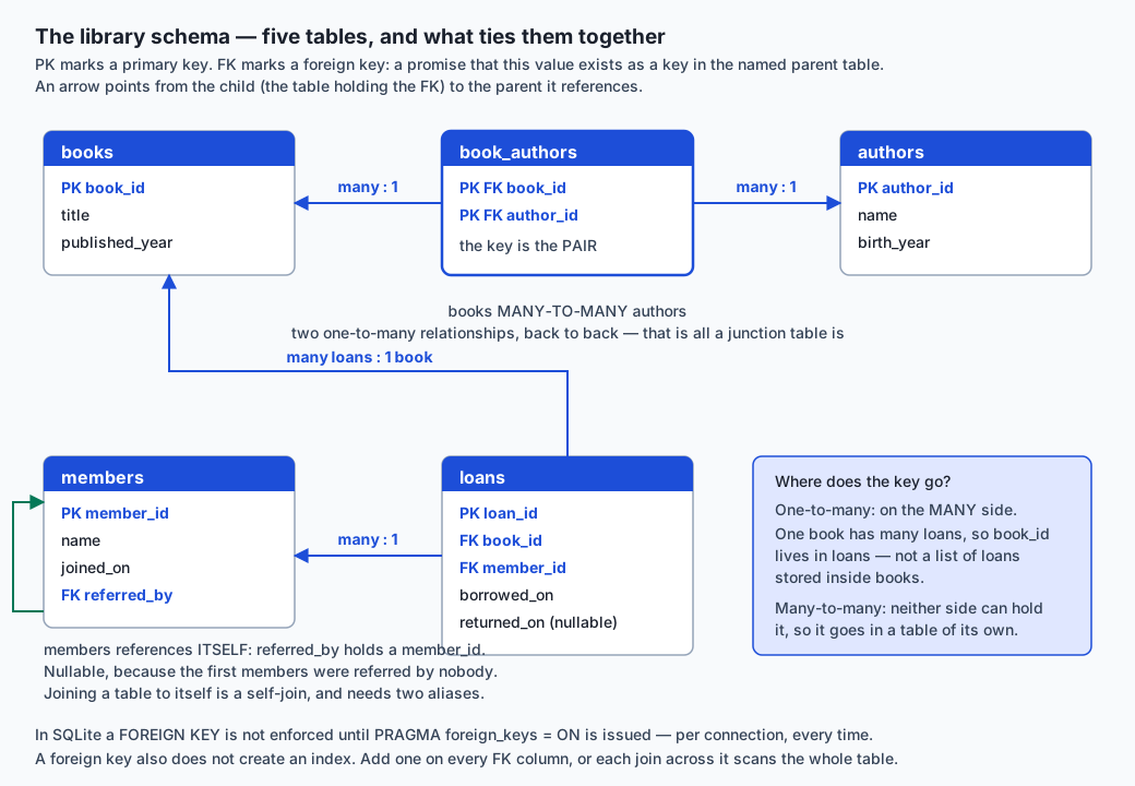
Read it as three separate patterns, because that is all there ever is.
One-to-many: the key goes on the many side
One book has many loans. One member has many loans. The rule is unvarying and it is worth saying out loud because people get it backwards: the foreign key lives on the “many” side.
CREATE TABLE loans (
  loan_id     INTEGER PRIMARY KEY,
  book_id     INTEGER NOT NULL REFERENCES books(book_id),
  member_id   INTEGER NOT NULL REFERENCES members(member_id),
  borrowed_on TEXT    NOT NULL,
  returned_on TEXT
);
book_id sits in loans, not a list of loans inside books. The reason is that a column holds one value. If you tried to put the relationship on the “one” side you would need a list in a cell, and the moment you have a list in a cell you have lost the ability to index it, join on it, or constrain it — you have a text field that happens to contain commas.
Many-to-many: it needs a table of its own
A book has several authors; an author has several books. Neither side can hold the key. So the relationship becomes a table:
CREATE TABLE book_authors (
  book_id   INTEGER NOT NULL REFERENCES books(book_id)     ON DELETE CASCADE,
  author_id INTEGER NOT NULL REFERENCES authors(author_id) ON DELETE RESTRICT,
  PRIMARY KEY (book_id, author_id)
);
Two details earn their place. The primary key is the pair, which is what makes it impossible to attach the same author to the same book twice — a constraint you would otherwise have to enforce in application code and would eventually get wrong. And the two ON DELETE clauses differ on purpose: deleting a book should remove its authorship rows (CASCADE), but deleting an author who still has books should be refused (RESTRICT), because it is almost certainly a mistake.
A junction table is not a special kind of object. It is two one-to-many relationships back to back, which is why joining across it always takes two JOIN clauses.
The join itself, row by row
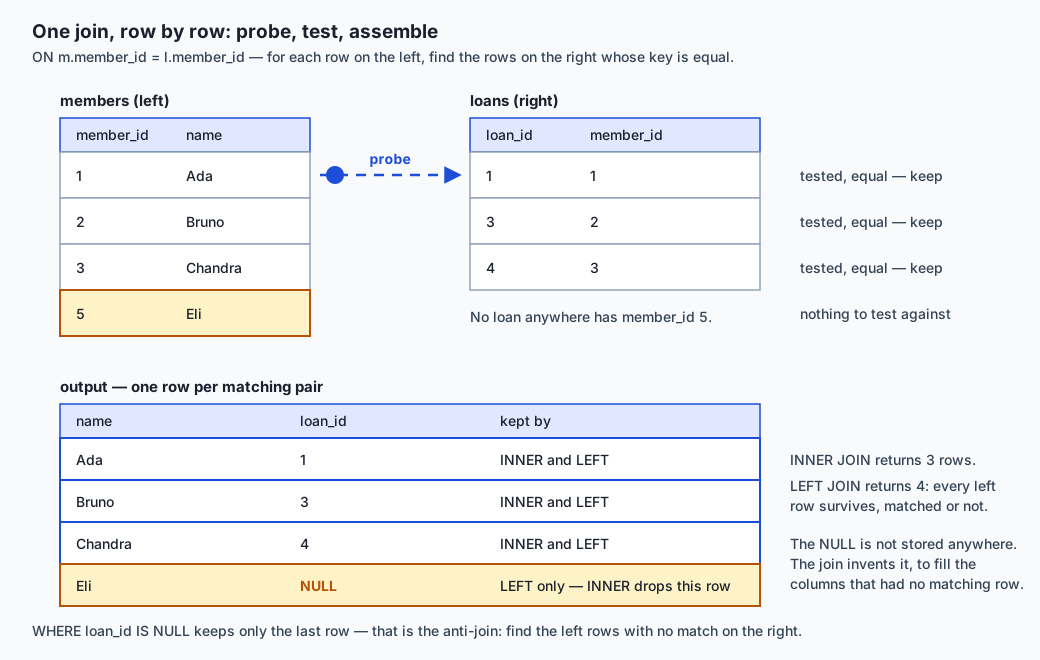
The mechanics, stated once and precisely. For each row on the left, the database finds every row on the right where the predicate is true, and emits one output row per matching pair. Three consequences follow, and all three surprise people:
- A left row matching three right rows produces three output rows. Joining does not preserve your row count.
- A left row matching nothing produces no output row under
INNER JOIN. - Under
LEFT OUTER JOIN, that unmatched left row produces one output row, with every right-hand column set to NULL.
That NULL is worth pausing on. It is not stored anywhere. No table contains it. The join invents it, on the spot, to fill the columns that had no matching row. This is why yesterday’s three-valued logic matters so much today: those manufactured NULLs then flow into every WHERE clause and every aggregate downstream, and they behave exactly as Day 86 said they would.
The join types, and exactly which rows survive
| Join type | Left rows with a match | Left rows with no match | Right rows with no match | Row count on the lab’s data |
|---|---|---|---|---|
INNER JOIN | kept, one row per pair | dropped | dropped | 7 book-author pairs |
LEFT OUTER JOIN | kept, one row per pair | kept, right columns NULL | dropped | 8 (adds Knuth) |
RIGHT OUTER JOIN | dropped if unmatched | dropped | kept, left columns NULL | mirror of the above |
FULL OUTER JOIN | kept | kept, right NULL | kept, left NULL | union of both |
CROSS JOIN | every left row paired with every right row | n/a — no predicate | n/a | 4 × 7 = 28 |
Two practical notes. LEFT and RIGHT are mirror images, so RIGHT JOIN is never necessary — swap the table order and use LEFT. Most working SQL contains almost no RIGHT JOIN, and that is a readability decision rather than a technical one: it is easier to reason about a query where the table you care about is always named first. And SQLite gained RIGHT and FULL OUTER JOIN only in version 3.39.0 (2022); it had LEFT from the beginning, which tells you which one people actually needed.
The anti-join: LEFT JOIN plus IS NULL
Memorise this shape. It answers every “which ones have none?” question you will ever be asked.
SELECT a.author_id, a.name
  FROM authors AS a
  LEFT JOIN book_authors AS ba ON ba.author_id = a.author_id
 WHERE ba.author_id IS NULL;
Real output from the lab:
author_id  name
---------  ---------------
7          Donald E. Knuth
The logic in one sentence: keep every author, then keep only the ones where the right-hand side came back NULL — which can happen for exactly one reason, that there was nothing to match. The same shape finds the books never borrowed (104 · The Practice of Programming) and the members who have never borrowed (Eli Nakamura).
Joins with GROUP BY, and the zero-count trap
Now the mistake almost everybody makes at least once. Count each member’s loans:
SELECT m.name, count(l.loan_id) AS loans
  FROM members AS m
  LEFT JOIN loans AS l ON l.member_id = m.member_id
 GROUP BY m.member_id, m.name;
member loans
-------------- -----
Ada Okafor 2
Bruno Salgado 2
Chandra Iyer 1
Dana Whitfield 1
Eli Nakamura 0Two separate decisions had to be right to get that zero, and getting either wrong produces a plausible, wrong report.
The join must be LEFT. With INNER JOIN, Eli Nakamura is not in the output at all — she has no loans, so she has no rows to be grouped. A report of “loans per member” that silently omits the members with no loans is precisely backwards, because those are the members the report was probably commissioned to find.
The count must be of a right-hand column. Switch count(l.loan_id) to count(*) and Eli’s row reads 1:
=== 7b. count(*) instead of count(l.loan_id) — the wrong answer ===
member          loans_wrong
--------------  -----------
Eli Nakamura    1
count(*) counts rows, and the NULL-extended row the outer join manufactured for her is still a row. count(l.loan_id) counts non-NULL values of that column, and aggregate functions skip NULLs — so it correctly reports zero. Yesterday’s lesson on NULL semantics, arriving with a bill.
ON versus WHERE, which is genuinely subtle
This is the one to slow down for. On an inner join, a predicate in ON and the same predicate in WHERE give identical results, and you can move it around freely. On an outer join they are completely different, because the outer join’s NULL-filling happens after ON and before WHERE.
Same question — “for each member, which books do they currently have out?” — written both ways.
Predicate in ON:
SELECT m.name, l.loan_id
  FROM members AS m
  LEFT JOIN loans AS l
         ON l.member_id = m.member_id
        AND l.returned_on IS NULL;
member loan_id
-------------- -------
Ada Okafor 2
Bruno Salgado 6
Chandra Iyer 4
Dana Whitfield
Eli NakamuraFive members, five rows. Correct.
The same predicate moved to WHERE:
member         loan_id
-------------  -------
Ada Okafor     2
Bruno Salgado  6
Chandra Iyer   4
Eli Nakamura
Four rows — and it is wrong in both directions at once, which is what makes it such a good example.
Dana Whitfield has vanished. She is a member in good standing who has returned everything she borrowed. Her rows were never NULL-extended, because she does have loans — they simply all carry a returned_on date. So every one of her rows failed the WHERE test, and with no surviving row she disappeared from the result entirely. The outer join did its job; the filter then undid it.
Eli Nakamura is still there — showing an empty loan_id, as though she had a book out. She has never borrowed anything in her life. Her row was NULL-extended by the outer join, and returned_on IS NULL is perfectly true of a manufactured NULL, so the filter kept her. A false positive dressed as a result.
One misplaced predicate; a member wrongly dropped and a member wrongly kept. The rule to carry away:
ONdecides what counts as a match. Filters on the right-hand table belong here.WHEREfilters the finished result. Filters on the left-hand table belong here.- The exception that proves it:
WHERE right.key IS NULLis deliberate, and is the anti-join above. It works because it collapses the outer join down to the unmatched rows.
Self-joins
A table joined to itself, with two aliases so the query can tell the copies apart:
SELECT m.name AS member, r.name AS referred_by
  FROM members AS m
  LEFT JOIN members AS r ON r.member_id = m.referred_by;
member referred_by
-------------- -------------
Ada Okafor
Bruno Salgado Ada Okafor
Chandra Iyer Ada Okafor
Dana Whitfield Bruno Salgado
Eli NakamuraLEFT matters here for the same reason as always: with INNER JOIN, the two members nobody referred disappear and five rows become three.
Three or more tables
Joins chain. Each JOIN adds one table and one predicate, and the rule of thumb is that N tables need at least N−1 join conditions. Drop one and the result multiplies: the lab’s test suite asserts that removing a single condition from the three-table books-authors join turns 7 correct rows into 49.
SELECT m.name, b.title, a.name
  FROM loans        AS l
  JOIN members      AS m  ON m.member_id  = l.member_id
  JOIN books        AS b  ON b.book_id    = l.book_id
  JOIN book_authors AS ba ON ba.book_id   = b.book_id
  JOIN authors      AS a  ON a.author_id  = ba.author_id
 WHERE l.returned_on IS NULL;
Three loans are outstanding. This returns four rows, because one of the books has two authors and each gets a row. That is not a bug and SELECT DISTINCT is usually the wrong fix, because it hides the question instead of answering it. Decide what one output row is supposed to mean. If it means “one loan”, do not join to authors; aggregate them with group_concat instead.
The SQLite fact that will bite you
Everything above assumed foreign keys mean something. In SQLite, by default, they do not.
Here is the proof, run in one sqlite3 session against the lab’s database — and it must be one session, because the setting is per connection:
--- 1. what the pragma says on a brand-new connection ---
setting              value
-------------------  -----
PRAGMA foreign_keys  0

--- 2. insert a loan for member 999, who does not exist ---
rows_inserted
-------------
1

--- 3. the orphan row is really there ---
loan_id  book_id  member_id
-------  -------  ---------
900      101      999
A loan belonging to a member who does not exist, inserted without complaint, into a schema that explicitly declares member_id INTEGER NOT NULL REFERENCES members(member_id).
The database will tell you, if you ask:
--- 4. and the database will tell you, if you ask it to check ---
table  rowid  parent   fkid
-----  -----  -------  ----
loans  900    members  0
Now enable enforcement and run the identical statement:
--- 5. clean up, enable enforcement, and try the identical insert ---
setting              value
-------------------  -----
PRAGMA foreign_keys  1

--- 6. the same statement, now rejected ---
Runtime error near line 43: FOREIGN KEY constraint failed (19)
Three properties of that pragma matter, and the SQLite documentation is explicit about all three:
- It is per connection. Every new connection starts with it off. Setting it in one shell session does nothing for the next.
- It is not stored in the database file. There is no way to mark a database as “always enforce”. The application must say so, every time it connects.
- It is a no-op inside a transaction, and — this is the part that wastes afternoons — attempting it does not return an error; it simply has no effect.
That third property has a nasty interaction with Python. The sqlite3 module opens transactions for you around writes, so a pragma issued after your first INSERT is silently ignored:
--- 2. the trap: the pragma is a no-op inside an open transaction ---
connection.in_transaction: True
pragma set, but it reads back as: 0
after commit(), setting it again reads back as: 1
the same insert now raises IntegrityError: FOREIGN KEY constraint failed
The habit that avoids it entirely is one line, issued first:
connection = sqlite3.connect("library.db")
connection.execute("PRAGMA foreign_keys = ON")   # first, before anything else
Building the join yourself
The join is not magic. It is one of a small number of algorithms, and the planner picks between them. Here are the two that matter, in plain Python over lists of dictionaries.
The nested-loop join. The obvious one: for every left row, scan every right row.
def nested_loop_join(left, right, left_key, right_key):
    pairs, comparisons = [], 0
    for left_row in left:
        for right_row in right:
            comparisons += 1
            if left_row[left_key] == right_row[right_key]:
                pairs.append((left_row, right_row))
    return pairs, comparisons
Cost: n × m. Six loans against five members is 30 comparisons.
The hash join. Index one side once, then look each row of the other side up.
def hash_join(left, right, left_key, right_key):
    index, operations = defaultdict(list), 0
    for right_row in right:              # build phase
        operations += 1
        index[right_row[right_key]].append(right_row)
    pairs = []
    for left_row in left:                # probe phase
        operations += 1
        for right_row in index.get(left_row[left_key], ()):
            pairs.append((left_row, right_row))
    return pairs, operations
Cost: n + m. Six loans and five members is 11 operations. Real captured output:
nested-loop join: 6 rows, 30 key comparisons
hash join:        6 rows, 11 operations
  (6 x 5 = 30 against 6 + 5 = 11; the gap widens as the square)

nested-loop == SQL: True
hash        == SQL: True
nested-loop == hash: True
Both produce the same six rows, and both match what SQLite produces, exactly. The difference is entirely in the cost, and the shape of that difference is the whole point: at 6 × 5 it is 30 against 11, which is nothing. At 10,000 × 10,000 it is a hundred million against twenty thousand. One grows as the product; the other as the sum.
The outer join, in this vocabulary, is a two-line change — when a left row finds no matches, emit it anyway, paired with None:
matches = index.get(left_row[left_key], [])
if matches:
    pairs.extend((left_row, match) for match in matches)
else:
    pairs.append((left_row, None))
None is precisely what SQL calls NULL. That is the entire mechanism.
You can watch the real planner choose. EXPLAIN QUERY PLAN says SCAN when it will read every row and SEARCH when it will jump straight to the matching ones through an index:
--- inner join on an indexed foreign key ---
QUERY PLAN
|--SCAN l USING COVERING INDEX idx_loans_member
`--SEARCH m USING INTEGER PRIMARY KEY (rowid=?)

--- a cartesian product: two SCANs and nothing tying them together ---
QUERY PLAN
|--SCAN books
`--SCAN authors
The first is a nested-loop join where the inner scan has been replaced by an index lookup — which is why the index on every foreign key column matters so much, and why it is a genuine problem that declaring the foreign key does not create one. The second is your missing join condition, visible before you run the query.
An everyday analogy
Think of a hotel’s front desk on a busy evening.
The hotel keeps two ledgers. One lists guests: name, home address, loyalty number. The other lists stays: which room, which nights, what rate. The reason they are separate ledgers is the reason your data is in separate tables — a guest who comes four times a year should have their address written down once, not four times, because otherwise the evening they move house you have to find and correct four entries and you will miss one.
Each stay entry carries a guest number. That number is the foreign key, and it lives in the stays ledger — on the “many” side — because one guest has many stays.
A join is the receptionist working with both ledgers open. Someone asks “who is in room 402 tonight?” She finds the stay, reads the guest number, and looks that number up in the guest ledger. Two ledgers, one answer, assembled on the spot and not written down anywhere.
The join types are what she does when a lookup fails.
Inner join: she is asked to list every occupied room with the guest’s name, and only reports rows where both halves were found.
Left outer join: she is asked to list every guest on the loyalty programme with tonight’s room, if any. Guests not staying tonight still appear — with the room column blank. That blank is the NULL, and notice it is not written in either ledger. It is a gap she creates in the act of putting them side by side.
The anti-join: “which loyalty members are not staying tonight?” She goes down the full guest list and reports only the ones whose room came back blank. Every “who has none of these?” question is that shape.
The cartesian product: a new hire is told to “match the guests with the stays”, forgets to match on the guest number, and produces every guest paired with every stay. Two hundred guests and three hundred stays gives sixty thousand slips of paper, each individually plausible. The database does exactly this, just as fast and just as uncomplainingly.
ON against WHERE: the instruction “list every loyalty member, and their room if they are staying tonight” is ON — the tonight condition is part of what counts as a match. The instruction “list every loyalty member, then cross off the ones not staying tonight” is WHERE — and it is a different instruction, which produces a different list.
The foreign key is the desk’s standing rule that no stay may be recorded against a guest number not in the guest ledger. And now the analogy earns its keep for SQLite: the rule is printed in the staff handbook, but it is only actually applied if the receptionist on duty decides to check. Each new receptionist starts their shift not checking, and there is no way to write “always check” into the ledger itself — you have to tell each one, at the start of every shift. That is PRAGMA foreign_keys = ON, per connection, every time. Any stay slips recorded during a shift when nobody was checking are still sitting in the ledger, pointing at guests who never existed.
Where the analogy stops: a receptionist gets slower in a straight line as the ledgers grow, while a database can pick a smarter method — the hash join is the receptionist first sorting tonight’s stays into pigeonholes by guest number, so that each lookup is one glance rather than a scan of the whole ledger.
Examples in practice
Three shapes you will actually write, using the tools as they are used.
Reporting on absence, in SQLite. The most valuable query shape in this lesson, because the answer is not visible in any single table:
SELECT b.book_id, b.title
  FROM books AS b
  LEFT JOIN loans AS l ON l.book_id = b.book_id
 WHERE l.loan_id IS NULL;
book_id title
------- ---------------------------
104 The Practice of ProgrammingThe acquisitions budget question — “what did we buy that nobody wants?” — is this query, and no amount of querying books alone will answer it.
A retrieval system tying a chunk back to its source, in PostgreSQL. This is the shape from the opening, written out. The vector search finds candidate chunks; the join supplies everything that makes them usable:
SELECT c.chunk_text,
       d.title,
       d.updated_at,
       d.version
  FROM chunks AS c
  JOIN documents AS d ON d.doc_id = c.doc_id
  JOIN acl       AS p ON p.doc_id = d.doc_id
 WHERE p.group_id = $1
   AND d.superseded_by IS NULL
 ORDER BY c.embedding <=> $2
 LIMIT 10;
Two of those joins are the security boundary. Remove the acl join and the query still runs, still returns ten plausible chunks, and now returns them to anybody. That is the concrete form of “a join can create — or fail to enforce — a disclosure that none of its inputs describes”.
Measuring N+1 rather than repeating the slogan. The lab answers one question two ways over 500 members and 2,000 loans, and reports real numbers:
N+1 loop:  501 queries      0.79 ms
one join:    1 queries      0.44 ms

same answer: True
Look honestly at that. 501 queries against 1 — a 500-fold difference in query count — produced a difference of about 0.35 milliseconds. Not 500-fold. Under 2×.
That is not an argument for writing N+1 loops, but it is an argument against reciting the rule without understanding it. The cost of a query is dominated by what surrounds it, and in an embedded database a query is a function call inside your own process. SQLite’s own documentation makes this argument at length on its page The N+1 Query Problem, and it is worth reading precisely because it contradicts advice you will hear repeated with great confidence. Across a network, each of those 501 queries is a round trip — at a very ordinary 1 ms, that is half a second against essentially nothing, and the rule is entirely right. The correct answer depends on a fact about your deployment, not on a rule about joins. Timings vary by machine and by run; the query counts do not, which is why the lab asserts the counts.
Implications: security, privacy, performance, scalability, and cost
Privacy: the join is the disclosure. Each table in the lab is fairly harmless alone. books is a catalogue. members is a mailing list. loans is integers and dates. The join produces “this named person read this named book on this date” — which is exactly the record that reading-privacy protections exist for. A join can create a disclosure that none of its inputs contains, so the unit to reason about when deciding who may see what is the query, not the table. This generalises well beyond libraries: it is the whole of the re-identification problem.
Security: foreign keys are integrity, not access control. They stop a loan pointing at a nobody. They do not authenticate, authorise, or protect the file — anyone who can read the database file can read every row, because it is an ordinary file with ordinary permissions and no encryption. Protection is filesystem permissions, disk encryption, or not storing it.
Security: parameterise, and know the one thing you cannot. Every query today is a literal you wrote, so there is nothing to inject. The moment a value comes from outside, use a placeholder — WHERE name = ? with the value passed separately — because that value never reaches the parser at all. The exception worth knowing: table and column names cannot be parameterised. If one ever comes from outside your program, check it against a hard-coded allow-list.
Performance: index every foreign key. Declaring the key creates no index. Without one, each join across it is a full scan, and the difference is exactly the nested-loop-versus-hash gap from earlier — cost growing as the product rather than the sum.
Performance: the cartesian product is a denial of service. Two 10,000-row tables joined without a condition is 100 million rows, and the database will honestly try. EXPLAIN QUERY PLAN shows it as two bare SCANs before you run anything, and a LIMIT on exploratory queries costs nothing.
Scalability: joins are the thing that gets hard first. A join needs both sides reachable, which is why they are cheap on one machine and expensive across a network, and why distributed databases put so much effort into avoiding them. It is also the honest reason document databases became popular: they trade the anomalies back for not having to join. That is a real trade, in both directions.
Cost: normalization moves cost from writes to reads, and it is usually right. Normalized means write once, read with a join. Denormalized means write many times, read directly. The second is faster to read and pays with the three anomalies plus the questions you can no longer ask. Denormalize deliberately, when you have measured, and write down what will keep the copies in step.
Alternatives: free, open source, and commercial
The relational model is close to universal, so most of this is portability rather than genuine alternatives — with one real exception at the end.
SQLite — free, public domain. Today’s tool, and the right default for anything embedded, single-machine, or under a few hundred gigabytes. Choose it when you want zero administration and a database that is one file you can copy. Full inner, left, cross and self joins; RIGHT and FULL OUTER JOIN since 3.39.0 (2022). The catch is today’s headline: foreign keys are off by default and must be enabled per connection. No server to install, no cost, no paid tier.
PostgreSQL — free, open source (PostgreSQL licence); paid only as hosting. Choose it when more than one process writes concurrently, when you want strict types, or when you need FULL OUTER JOIN, window functions and CTEs used heavily. Foreign keys are enforced by default — there is no pragma and no opt-in; a violating insert is rejected from the first day. The join syntax is identical to what you have written today. Two differences worth knowing: FULL OUTER JOIN has been supported for far longer, and Postgres will genuinely choose between nested-loop, hash and merge joins based on statistics, which you can inspect with EXPLAIN ANALYZE. Worked example — the same anti-join, unchanged:
SELECT a.author_id, a.name
  FROM authors a
  LEFT JOIN book_authors ba ON ba.author_id = a.author_id
 WHERE ba.author_id IS NULL;
Free to run yourself forever; managed hosting is where money appears, and prices change often enough that you should read the provider’s current page rather than trust a figure written here.
MySQL / MariaDB — free, open source (GPL-2.0; MySQL also sold commercially by Oracle); MariaDB is the community fork. Choose it for the enormous ecosystem, or because your host offers it and nothing else. Foreign keys are enforced by default — but with a real caveat that has bitten a generation: only on the InnoDB storage engine. The older MyISAM engine parses FOREIGN KEY clauses and silently ignores them, which is the same trap as SQLite’s pragma wearing different clothes. InnoDB has been the default since MySQL 5.5, so this mainly matters for inherited schemas. Joins are standard; MySQL lacked FULL OUTER JOIN for a long time and the usual workaround is a UNION of a left and a right join.
DuckDB — free, open source (MIT). An embedded database like SQLite, but column-oriented and built for analytics. Choose it when your joins are large aggregations over files rather than small lookups — it will join Parquet or CSV files directly, without loading them first:
SELECT a.name, count(*)
  FROM 'books.parquet' b
  JOIN 'book_authors.parquet' ba ON ba.book_id = b.book_id
  JOIN 'authors.parquet' a ON a.author_id = ba.author_id
 GROUP BY a.name;
Same join syntax, and it is genuinely much faster on large analytical joins because it processes columns in batches rather than rows one at a time. It is not a replacement for SQLite in a transactional application. No paid tier for the database itself.
No database at all: dictionaries in Python. Entirely legitimate for small, in-memory, one-off work — and it is exactly what you implement in the lab. Choose it when the data fits comfortably in memory, the task runs once, and adding a database would be more machinery than the problem deserves.
by_member = {m["member_id"]: m for m in members}
for loan in loans:
    member = by_member.get(loan["member_id"])       # your hash join
    name = member["name"] if member else None       # your LEFT JOIN
What you give up, and it is worth being honest: no constraints, no durability, no concurrent access, no query planner, and every one of the three anomalies is now your problem to avoid by hand. Free, in that there is nothing to install; expensive in maintenance the moment the data outgrows the assumption.
And the trap that lives in that alternative: N+1 queries. The moment your “no database” instinct meets a real database, it turns into a loop that queries per row:
for member in connection.execute("SELECT * FROM members"):
    loans = connection.execute(
        "SELECT count(*) FROM loans WHERE member_id = ?", (member[0],)
    ).fetchone()
That is 1 + N queries where a single LEFT JOIN ... GROUP BY would do. As the lab measures, the penalty on an embedded database is real but small — 501 queries against 1 cost about 0.79 ms against 0.44 ms — and across a network it is one round trip per row, which is the difference between imperceptible and unusable. Read SQLite’s own page on this; it argues the case for the embedded side honestly, and a nuance you understand is worth more than a rule you repeat.
Comparison with related concepts
| Concept | What it does | How it differs from a join |
|---|---|---|
UNION | Stacks two result sets vertically | A join adds columns to rows; UNION adds rows. Requires the same column count and compatible types |
Subquery in WHERE | Filters using another query’s results | Returns nothing from the inner table. WHERE id IN (SELECT ...) filters; a join brings the columns along |
EXISTS | Tests whether a matching row exists | Semi-join: filters without multiplying rows. Often the better choice when you only want “is there one?” and a join would duplicate |
NOT EXISTS | Tests that no matching row exists | The other spelling of the anti-join. Safer than NOT IN, which returns nothing at all if the subquery yields a single NULL |
CTE (WITH) | Names an intermediate result | Structuring, not matching. Frequently wraps joins to make them readable |
| Window function | Computes across related rows without collapsing them | Neither combines tables nor removes rows; adds a column computed over a partition |
| Foreign key | Constrains values to exist in a parent | A promise about data; the join is the operation. Neither implies the other |
| Index | Speeds up finding rows by a column | Changes the algorithm a join can use; does not change its result |
VIEW | A stored query, often a join | Saves the query text, not the result. Runs afresh each time |
| Denormalization | Deliberately storing data pre-joined | The trade you make to avoid joining, paid for with the three anomalies |
The one worth dwelling on is NOT IN against NOT EXISTS, because it is where today’s material collides hardest with yesterday’s. WHERE member_id NOT IN (SELECT member_id FROM loans) gives the right answer on the lab’s data — the test asserts it — but only because no loans.member_id is NULL. Let a single NULL into that subquery and NOT IN returns no rows at all, because x NOT IN (1, 2, NULL) evaluates to unknown rather than true. NOT EXISTS and the LEFT JOIN ... IS NULL idiom are both immune. This is the most common way Day 86’s three-valued logic ruins somebody’s afternoon.
When to use it — and when not to
Use a join when the fact you need lives in another table — which, in a properly normalized schema, is most of the time. Use LEFT JOIN specifically whenever the answer needs to include things that have none of something: the customers who never ordered, the members who never borrowed, the documents with no permissions row.
Use EXISTS instead when you only want to know whether a match exists and do not need columns from the other table. It expresses the intent better and cannot accidentally multiply your rows.
Do not join when you only need a key you already have. If loans.member_id is what you want, take it from loans. Joining to members to read a column you were already holding is a common reflex and pure cost.
Do not use a join to enforce access control on its own. A missing acl join is a query that runs perfectly and returns data to the wrong person. Filter at a level where forgetting it fails closed rather than open.
Do not normalize to the last drop for its own sake. Normalization is a tool for eliminating anomalies, not a score. If a lookup table of three values that never change is making every query longer, inline it and write down why.
Denormalize deliberately, and only with a plan for keeping the copies in step. A cached loan_count on members is a perfectly reasonable engineering decision — provided you can name every path that changes a loan and say how each one updates the count. If you cannot, you have chosen the update anomaly on purpose.
And when the data does not fit the relational model at all, notice that rather than fighting it. Deep hierarchies, wildly variable documents and pure key-value workloads are all things other stores do better. That is a real trade with a real cost — you give up the constraints and the ad-hoc queries — but it is a choice, not a failure.
Where this goes next in AI work
Come back to the opening, now that the mechanism is in place.
A retrieval-augmented system stores chunks and their embeddings. The chunk is the least important row in the design. Around it sit the document it came from, the version of that document, the access-control entry deciding who may see it, the ingestion record saying when it was last refreshed, and the evaluation results saying whether it has ever produced a good answer. Every one of those is a join away.
That is not incidental plumbing; the joins are where the correctness lives.
Miss the superseded_by IS NULL condition and your assistant confidently quotes a policy that was withdrawn eight months ago — with a citation, which makes it worse, because a citation is what people use to decide whether to check. Miss the permissions join and it quotes one team’s confidential document to another team. Get the freshness join wrong and it cannot tell you how stale its answer is, which means it cannot tell you when not to trust it.
And the anti-join is the shape of every quality question worth asking about a pipeline. Which documents were ingested but never embedded — LEFT JOIN embeddings ... WHERE embedding_id IS NULL? Which embeddings point at a document that has since been deleted? Which of your evaluation questions has no retrieved chunk at all, meaning the retriever failed silently rather than badly? Every one of those is LEFT JOIN plus IS NULL, and every one of them is invisible if you only ever query one table.
One more, because it connects directly to today’s headline. If you build that pipeline on SQLite — and for a first RAG prototype you very likely will — and you never issue PRAGMA foreign_keys = ON, then chunks pointing at deleted documents will accumulate silently, for months. Your retriever will return them. They will have no title, no date, and no permissions, and your code will fill those gaps with defaults. Nothing will error. This is not hypothetical: it is the default behaviour of the most widely deployed database in the world, and today you proved it in six lines.
Knowledge check
Try these from memory before looking back.
- Name the three anomalies a single wide table causes, and for each one give a concrete example of the damage. Which of the three is most dangerous, and why is “it raises no error” the answer?
- Where does the foreign key go in a one-to-many relationship, and why can it not go on the other side? Answer in terms of what a column can hold.
- Why does a many-to-many relationship need a third table? What is its primary key, and what does that key prevent?
- State exactly which rows an
INNER JOINkeeps and which aLEFT OUTER JOINkeeps. Where does the NULL in an outer join’s right-hand columns come from — which table is it stored in? - Write the
LEFT JOINplusIS NULLidiom from memory and say what it finds. Why does it work — what is the only circumstance that can make the right-hand column NULL? - A per-member loan count returns 1 for a member who has borrowed nothing. Name the two separate mistakes that could cause it, and give the fix for each.
- Explain the difference between putting
l.returned_on IS NULLinONand inWHEREon aLEFT JOIN. Using the lesson’s data, name the member wrongly dropped and the member wrongly kept, and say why each happens. - What is
PRAGMA foreign_keysset to on a brand-new SQLite connection? Give the three properties of that setting, and describe the trap that makes it silently fail in Python. - Compare a nested-loop join and a hash join: how does each work, what does each cost, and what does the planner print in
EXPLAIN QUERY PLANwhen it has chosen an indexed nested loop? - Why does declaring a foreign key not make your joins fast? What must you do as well, and what happens if you do not?
Hands-on exercise
The Day 87 lab, Connecting the Tables, runs today’s argument as a sequence you execute. Work in the lab directory; every command below is run from there. Nothing needs installing and nothing touches the network.
Start with the whole harness:
bash tests/run_tests.sh
echo "exit code: $?"
Then walk the argument in order. First the mistake:
sqlite3 anomalies.db < examples/01_wide_table.sql
rm -f anomalies.db
Then the split, and the fact worth remembering from today. The foreign-key proof must be one sqlite3 session, because the pragma is per connection — two invocations would prove nothing:
rm -f library.db
sqlite3 library.db < examples/02_schema.sql
sqlite3 library.db < examples/03_seed.sql
sqlite3 library.db < examples/04_foreign_keys.sql; echo "exit: $?"
Then every join type, the two hand-written join algorithms, the Python pragma trap, the measured N+1 comparison, and the planner:
sqlite3 library.db < examples/05_joins.sql
python3 examples/06_join_from_scratch.py library.db
python3 examples/07_foreign_keys_python.py
python3 examples/08_n_plus_one.py
sqlite3 library.db < examples/09_query_plans.sql
Then do it yourself. starter/ holds nine numbered exercises. Six are SQL queries that run as they stand and are each wrong in one specific, named way — the comment above each says what is wrong, what to change, and which check verifies it. Three are the join algorithms in Python, and that file reports its own pass and fail lines.
bash starter/01_build.sh
sqlite3 starter/library.db < starter/02_exercises.sql
python3 starter/03_join_from_scratch.py
Expected output
The harness ends with a real captured line:
75 checks, 0 failure(s).The foreign-key proof prints PRAGMA foreign_keys 0 on a fresh connection, then inserts a loan for member 999 successfully (rows_inserted 1), then shows the orphan row, then finds it with PRAGMA foreign_key_check, then prints PRAGMA foreign_keys 1, then fails the identical insert with Runtime error near line 43: FOREIGN KEY constraint failed (19) — and exits non-zero, on purpose.
The Python version adds the trap:
connection.in_transaction: True
pragma set, but it reads back as: 0
after commit(), setting it again reads back as: 1
the same insert now raises IntegrityError: FOREIGN KEY constraint failed
The joins produce 7 book-author pairs from the inner join, 28 from books CROSS JOIN authors, 8 from the left join of authors to books, and exactly one row each for the three anti-joins (Donald E. Knuth, 104 · The Practice of Programming, Eli Nakamura). Loans per member reads Ada 2, Bruno 2, Chandra 1, Dana 1, Eli 0 — and switching to count(*) reports 1 for Eli, while switching to an inner join drops her row entirely. Moving returned_on IS NULL from ON to WHERE takes the result from 5 rows to 4, losing Dana Whitfield and keeping Eli Nakamura.
The hand-written joins print:
nested-loop join: 6 rows, 30 key comparisons
hash join:        6 rows, 11 operations

nested-loop == SQL: True
hash        == SQL: True
nested-loop == hash: True
And the starter reports 0 of 3 exercises complete. with exit 1 before you begin, 3 of 3 with exit 0 when you are done.
Validate your work
bash tests/run_tests.shends with75 checks, 0 failure(s).and exits 0.- The wide table leaves two different spellings of one author’s name, having raised no error, and zero rows mentioning Brooks after his only book is withdrawn.
examples/04_foreign_keys.sqlinserts the orphan successfully with the pragma off, rejects the identical statement with it on, and exits non-zero.- The inner join across the junction returns 7 rows;
books CROSS JOIN authorsreturns 28; dropping one condition from the three-table join returns 49. - The left join of authors to books returns 8 rows, the extra being Donald E. Knuth with both right-hand columns NULL.
- The three anti-joins each find exactly one row, and they are the three named above.
- Loans per member gives Eli 0 with
count(l.loan_id), 1 withcount(*), and no row at all withJOIN. - Moving the predicate from
ONtoWHEREgoes from 5 rows to 4 — Dana dropped, Eli kept. - The self-join keeps 5 members with
LEFT JOINand 3 withJOIN; the four-table join returns 4 rows for 3 outstanding loans. 06_join_from_scratch.pyprintsTrueon all three comparison lines and exits 0.08_n_plus_one.pyprints501and1queries withsame answer: True.- After the harness finishes,
ls library.dbfinds nothing — it built and removed everything in a temporary directory.
Troubleshooting
The lab’s troubleshooting.md has the full list. The ones you are most likely to meet: no such table, which usually means SQLite silently created an empty database from a mistyped filename rather than complaining — check .tables before assuming your schema failed. A FOREIGN KEY constraint failed that never happens, which is the pragma being off; remember it is per connection, is not stored in the file, and must be reissued every time. A pragma that reads back as 0 in Python, which is it being ignored inside an open transaction — issue it as the first statement after connecting. A join returning far more rows than either table has, which is a missing join condition; N tables need at least N−1 of them. A LEFT JOIN behaving like an inner one, which is a predicate that has drifted into the WHERE clause. And counts of 1 where you expected 0, which is count(*) counting the NULL-extended row.
Common mistakes
- Forgetting a join condition. The result multiplies instead of erroring. Count your
ONclauses: N tables, at least N−1. - Using
INNER JOINfor a report about absence. The rows you are looking for are exactly the ones an inner join removes. count(*)after aLEFT JOIN. Counts the manufactured NULL row as 1. Count a right-hand column.- A right-table predicate in
WHEREon an outer join. Silently collapses it to an inner join — and, as the lab shows, can wrongly keep rows at the same time as wrongly dropping them. - Assuming SQLite enforces your foreign keys. It does not, until you say so, on every connection.
- Setting the pragma after your first write in Python. It is a documented no-op inside a transaction and returns no error.
- Expecting a foreign key to create an index. It does not. Every join across an unindexed key is a full scan.
SELECT DISTINCTto hide duplicate rows from a many-to-many. It hides the question. Decide what one output row should mean.NOT INwith a subquery that can contain NULL. Returns nothing at all, silently. UseNOT EXISTSor theLEFT JOIN ... IS NULLidiom.- Joining to a table to read a column you already have. Pure cost.
Practice assignment
Design and build a small relational schema of your own, from data you actually have — the podcasts you subscribe to and their episodes, your photo library and its tags, the repositories you have starred and their languages, a reading list.
Start by writing the wide table. One table, everything in it, deliberately denormalized. Then commit all three anomalies against it, in SQL, and capture the output. Rename something and miss a row. Try to insert an entity that has no child rows yet and find there is nowhere to put it. Delete a row and watch a second fact disappear with it. You will understand the rest far better for having broken it yourself first.
Then normalize it. At least four tables, with at least one one-to-many, at least one many-to-many with a proper junction table keyed on the pair, and at least one nullable foreign key. Write the schema with real REFERENCES clauses, sensible ON DELETE behaviour, and an index on every foreign key column — then say in a comment why that index is not created for you.
Then prove the constraint is real. Insert a deliberate orphan with PRAGMA foreign_keys off and show it succeeding. Enable it, run the identical statement, and capture the rejection. Save both outputs; that pair of captures is the most valuable artefact in the assignment.
Then write six queries, and for each one write down the answer you expect before you run it:
- An inner join across your junction table.
- A left outer join that keeps rows with no match.
- An anti-join finding entities with none of something.
- A per-group count where at least one group must correctly show zero.
- A join across three or more tables.
- A query where you deliberately move a predicate from
ONtoWHEREon an outer join, and record how the result changes.
Where any answer differs from your prediction, write down why. Those are the ones you actually learned from.
Your deliverable is the schema, the two anomaly captures, the six queries with their real output, and one paragraph on the privacy question: name a join over your own schema that produces a record more sensitive than any of its input tables. Every schema has one. Finding it is the point.
Extension challenge
Three extensions, each forcing a judgement rather than more typing.
Implement a sort-merge join, and work out when a planner would choose it. Add a third algorithm to the lab’s Python file: sort both sides by the join key, then walk them with two pointers, advancing whichever is behind. Count its operations alongside the nested-loop and hash versions. The interesting part is not the code, it is the analysis. Sorting costs n log n, so on the face of it a hash join should always win — and yet real planners choose merge joins constantly. Work out why, and the answer will lead you to a fact about indexes: an index is a sorted copy of a column, so if both sides are already indexed on the join key the sort is free and merge becomes the cheapest option available. Write down what that implies about which indexes to create.
Inherit a broken database, and find out what enabling the pragma does and does not do. With PRAGMA foreign_keys off, insert several orphan rows across different tables. Now answer three questions by experiment rather than by guessing. Does PRAGMA foreign_keys = ON retroactively reject the rows already there, or only future statements? What does PRAGMA foreign_key_check report, and is it enough to repair from? And — the one that matters — if you were handed a SQLite database that some application had been writing to for three years without ever enabling the pragma, what would you actually run, in what order, to find out how bad it is? Write that as a checklist. You will use it one day.
Do the N+1 arithmetic for a deployment, and let it change your answer. Take the lab’s measured numbers — 501 queries at 0.79 ms against 1 query at 0.44 ms, in-process — and recompute the same workload for a client-server database with a 1 ms network round trip, then again with a 20 ms one for a database in another region. Then read SQLite’s own page on the N+1 query problem and decide, in writing, which design you would choose for each of three deployments: an embedded database in a desktop application, a Postgres instance in the same datacentre, and a managed database three time zones away. State what changed between them. The point of the exercise is that the answer is not the same three times, and an engineer who knows why it differs is worth considerably more than one who has memorised the rule.
Quiz
Q1. A LEFT OUTER JOIN from members to loans is run against a library where one member has never borrowed anything. Which rows does the result contain?
- Every member who has at least one loan, one row per loan — the unmatched member is dropped
- Every member exactly once, with the loans columns holding the most recent loan
- Every loan, plus one row for each member, concatenated
- Every member, with one row per loan for those who have loans and a single row with NULL in every loans column for the member who has none
Show answer
Answer: D. Every member, with one row per loan for those who have loans and a single row with NULL in every loans column for the member who has none
A LEFT OUTER JOIN keeps every row from the left table regardless of whether it matched. Rows that matched produce one output row per matching pair — so a member with two loans produces two rows, and joining does not preserve your row count. The row that matched nothing survives exactly once, with every column that came from the right table set to NULL. That NULL is worth being precise about: it is not stored in any table. The join manufactures it on the spot to fill the columns that had no matching row, which is exactly why it then flows into every WHERE clause and aggregate downstream and behaves according to three-valued logic. Option 0 describes an INNER JOIN, which is precisely the join that removes the row you were looking for.
Q2. On a brand-new SQLite connection, you insert a row into a child table whose foreign key points at a parent row that does not exist. What happens?
- The insert is rejected with FOREIGN KEY constraint failed, because the REFERENCES clause is in the schema
- The insert succeeds, because SQLite disables foreign-key enforcement by default and it must be enabled separately for every connection
- The insert succeeds but SQLite writes a warning to stderr
- The insert succeeds only if the column is nullable; otherwise it is rejected
Show answer
Answer: B. The insert succeeds, because SQLite disables foreign-key enforcement by default and it must be enabled separately for every connection
SQLite gained foreign key enforcement in version 3.6.19 (14 October 2009), nine years after its first release, and because a decade of databases already existed that would break under it, the documentation states that constraints are "disabled by default (for backwards compatibility), so must be enabled separately for each database connection". The orphan row is inserted with no error and no warning. Three properties follow and all three catch people out: the setting is per connection, so every new connect() starts with it off; it cannot be stored in the database file, so the application must issue it every time; and it is documented as a no-op inside a transaction that "does not return an error; it simply has no effect". PRAGMA foreign_key_check will find orphans that are already there.
Q3. This query reports 1 for a member who has never borrowed anything: SELECT m.name, count(*) FROM members m LEFT JOIN loans l ON l.member_id = m.member_id GROUP BY m.member_id. Why?
- The LEFT JOIN is wrong; it should be an INNER JOIN
- GROUP BY always produces at least one row per group with a count of 1
- count(*) counts rows, and the NULL-extended row the outer join manufactured for that member is still a row — count(l.loan_id) would correctly report 0 because aggregates skip NULLs
- The member has a loan record that was deleted but not vacuumed
Show answer
Answer: C. count(*) counts rows, and the NULL-extended row the outer join manufactured for that member is still a row — count(l.loan_id) would correctly report 0 because aggregates skip NULLs
Two separate decisions have to be right to get a genuine zero, and this query got one of them wrong. The LEFT JOIN is correct and necessary — switching to INNER JOIN would drop the member from the report entirely, which is worse, because a "loans per member" report that silently omits the members with no loans is exactly backwards. The bug is count(*), which counts rows without looking at their contents, and the outer join produced one row for this member with every loans column NULL. Counting a column from the right-hand table instead — count(l.loan_id) — gives 0, because aggregate functions skip NULLs. This is Day 86's three-valued logic arriving with a bill.
Q4. You move the predicate l.returned_on IS NULL from the ON clause of a LEFT JOIN into the WHERE clause. On the lesson's library data the result goes from 5 rows to 4. What is wrong with the 4-row result?
- Nothing — ON and WHERE are interchangeable, and the shorter result is simply more concise
- It is missing one member, which is the only error
- It is wrong in both directions: it drops a member who has genuinely returned everything, and it keeps a member who has never borrowed at all, showing her as though she had a book out
- It returns the same members but in a different order
Show answer
Answer: C. It is wrong in both directions: it drops a member who has genuinely returned everything, and it keeps a member who has never borrowed at all, showing her as though she had a book out
On an INNER JOIN the two are interchangeable. On an OUTER JOIN they are not, because the NULL-filling happens after ON and before WHERE. Both failures show up here at once. Dana Whitfield disappears: she has loans, but all of them carry a returned_on date, so every one of her rows fails the WHERE test and she vanishes with no surviving row. Eli Nakamura survives: she has never borrowed anything, so the outer join manufactured a NULL-extended row for her, and returned_on IS NULL is perfectly true of a manufactured NULL — a false positive dressed as a result. The rule: ON decides what counts as a match, so filters on the right-hand table belong there; WHERE filters the finished result. The deliberate exception is WHERE right.key IS NULL, which is the anti-join and works precisely because it collapses the outer join down to the unmatched rows.
Q5. Why does a many-to-many relationship between books and authors require a third table?
- It does not; you can store a comma-separated list of author IDs in the books table
- Because a column holds one value, so neither side can hold the relationship — and the junction table's primary key is the pair, which is what prevents attaching the same author to the same book twice
- Because SQLite does not allow two foreign keys in the same table
- For performance only; a third table makes the join faster but is not logically required
Show answer
Answer: B. Because a column holds one value, so neither side can hold the relationship — and the junction table's primary key is the pair, which is what prevents attaching the same author to the same book twice
A one-to-many relationship is modelled by putting the foreign key on the many side — book_id lives in loans, not a list of loans inside books — and the reason is that a column holds one value. In a many-to-many, both sides are the many side, so neither can hold the key and the relationship gets a table of its own. Making its primary key the pair (book_id, author_id) is what makes it impossible to attach the same author to the same book twice, a constraint you would otherwise enforce in application code and eventually get wrong. A junction table is not a special kind of object: it is two one-to-many relationships back to back, which is why joining across it always takes two JOIN clauses. Option 0 is the trap: the moment you have a list in a cell you have lost the ability to index it, join on it, or constrain it.
Q6. A join between two tables of 10,000 rows each returns 100,000,000 rows. What has almost certainly happened, and what does EXPLAIN QUERY PLAN show?
- A missing or incorrect join condition, producing a cartesian product — the plan shows two bare SCANs with nothing tying them together
- A duplicate primary key in one of the tables
- The query needs an ORDER BY to deduplicate the output
- A LEFT JOIN was used where an INNER JOIN was needed
Show answer
Answer: A. A missing or incorrect join condition, producing a cartesian product — the plan shows two bare SCANs with nothing tying them together
100,000,000 is exactly 10,000 x 10,000, which is the signature of a cartesian product: every left row paired with every right row because nothing constrained the match. The rule of thumb is that N tables need at least N minus 1 join conditions, and dropping a single condition from a three-table join in the lab turns 7 correct rows into 49. EXPLAIN QUERY PLAN shows this before you run anything: SCAN means read every row and SEARCH means jump to the matching rows through an index, so a SCAN plus a SEARCH is an indexed nested-loop join while two bare SCANs is the product. This matters beyond correctness — at real scale the database will honestly try to produce all hundred million rows, which on a shared server is an outage caused by a query that looked fine in review.
Q7. Which pair of statements about foreign keys is true?
- A foreign key creates an index on the column, and performs the join for you when you query the parent table
- A foreign key creates an index but only in PostgreSQL, and it makes JOIN keywords unnecessary
- A foreign key requires the referencing column to be NOT NULL, and automatically cascades deletes
- A foreign key creates no index, so you must add one yourself or every join across it is a full table scan — and it does not perform any join; it only guarantees the join will find something
Show answer
Answer: D. A foreign key creates no index, so you must add one yourself or every join across it is a full table scan — and it does not perform any join; it only guarantees the join will find something
Both halves surprise people. Declaring book_id INTEGER REFERENCES books(book_id) builds no index on book_id, so every join across it — and every referential-integrity check on the child side — scans the whole table; the lab's schema adds the indexes explicitly with a comment saying why. And a foreign key is a constraint, not a traversal: you still write the JOIN, and the key only promises the join will find a matching parent. Two further non-promises: a nullable foreign key may be NULL, meaning "this row references nothing" (the lab's members.referred_by is exactly that), and delete behaviour is whatever the schema says — CASCADE, SET NULL or RESTRICT — not an automatic cascade.
Q8. A nested-loop join and a hash join over the same two tables return identical results. What is the difference between them?
- The hash join returns approximate matches, trading accuracy for speed
- The nested loop scans every right row for each left row, costing n times m; the hash join indexes the right side once and then probes it once per left row, costing n plus m
- The nested loop works only on sorted input; the hash join works on unsorted input
- They are the same algorithm under different names
Show answer
Answer: B. The nested loop scans every right row for each left row, costing n times m; the hash join indexes the right side once and then probes it once per left row, costing n plus m
Both are exact and both return the same rows — the lab asserts that the two hand-written implementations agree with each other and with SQLite, row for row. The entire difference is cost. The nested loop compares everything with everything: 6 loans against 5 members is 30 comparisons. The hash join has a build phase that touches each right row once and a probe phase that touches each left row once: 6 plus 5 is 11 operations. At that scale the gap is nothing, which is the point of measuring it there; at 10,000 by 10,000 it is a hundred million against twenty thousand, because one grows as the product and the other as the sum. This is the choice a query planner is making, and EXPLAIN QUERY PLAN lets you see which it took.
Glossary
- Join
- An operation that combines rows from two tables into one result, pairing each row on the left with the rows on the right that satisfy a condition you supply. Nothing is stored joined: the result is assembled when you ask and thrown away when you are done. A left row matching three right rows produces three output rows, so joining does not preserve your row count.
- Join predicate
- The condition in the ON clause that decides which pairs of rows belong together, usually an equality between a foreign key on one side and a primary key on the other. On an outer join it is not interchangeable with a WHERE clause: the predicate in ON decides what counts as a match, while WHERE filters the finished result after the NULL-filling has already happened.
- Primary key
- The column, or set of columns, that identifies a row uniquely within its table. In a junction table it is the pair of foreign keys together, which is what makes it impossible to record the same relationship twice.
- Foreign key
- A column whose values are required to appear as a primary key in another table. It promises that every non-NULL value here exists as a parent row, that you cannot insert a child pointing at a missing parent, and that deleting a parent with children follows whatever the schema says. It does not create an index, does not perform the join, and — in SQLite — does not enforce anything until PRAGMA foreign_keys is switched on.
- Referential integrity
- The property that every foreign-key value actually points at a row that exists, so the database contains no references to nothing. It is an integrity control rather than a security control: it stops a loan pointing at a member who does not exist, and stops nothing else. PRAGMA foreign_key_check reports where it has already been violated.
- Orphan row
- A child row whose foreign key points at a parent that does not exist. In SQLite these accumulate silently in any database written to by an application that never enabled foreign-key enforcement, because the insert that creates one succeeds with no error and no warning.
- Cardinality
- How many rows on one side of a relationship correspond to how many on the other: one-to-one, one-to-many, or many-to-many. It decides where the key goes. In a one-to-many the foreign key lives on the many side, because a column holds one value; in a many-to-many neither side can hold it, so the relationship needs a table of its own.
- Junction table
- A table whose only job is to record a many-to-many relationship, holding one foreign key to each side and keyed on the pair. Also called a bridge, link or associative table. It is not a special kind of object: it is two one-to-many relationships back to back, which is why joining across it always takes two JOIN clauses.
- Inner join
- The default join. Rows that satisfy the predicate come through, one output row per matching pair; rows on either side that match nothing are dropped. This is precisely why it is the wrong join for any question about absence — the rows you are looking for are the ones it removes.
- Outer join
- A join that keeps rows which matched nothing. LEFT keeps every row from the left table, filling the right-hand columns with NULL when there was no match; RIGHT is its mirror image and is rarely needed, since swapping the table order and using LEFT is easier to read; FULL keeps unmatched rows from both sides. The NULL an outer join produces is not stored in any table — the join manufactures it to fill columns that had no matching row.
- Anti-join
- The idiom for finding rows with no match: LEFT JOIN the other table, then keep only the rows where its columns came back NULL, which can happen for exactly one reason. Worth memorising as a unit, because it is the shape of every question about absence — which customers never ordered, which documents were never embedded, which books nobody has borrowed.
- Self-join
- A table joined to itself, with two distinct aliases so the query can tell the copies apart. It relates rows to other rows in the same table: employees to managers, members to whoever referred them, replies to the comment they answer. Use LEFT unless you specifically want to exclude the rows that reference nobody, because an inner self-join silently drops them.
- Cartesian product
- Every row of one table paired with every row of another, which is what a join with no condition produces — four books and seven authors give twenty-eight rows. Usually accidental, caused by a forgotten join condition, and the rule of thumb is that N tables need at least N minus 1 of them. At real scale it is a denial of service: two tables of ten thousand rows produce a hundred million, and the database will honestly try.
- Normalization
- Organising tables so that each is about one kind of thing and every fact is written down in exactly one place, eliminating the update, insertion and deletion anomalies. Developed by E. F. Codd through 1971 and 1972 as the first three normal forms. It moves cost from writes to reads: you store each fact once and pay a join to reassemble it.
- Update anomaly
- The failure where a fact stored in several rows is corrected in some of them and not others, leaving the database contradicting itself with no error raised. The most dangerous of the three anomalies precisely because it is silent: nothing marks which of the two values is the right one.
- Insertion anomaly
- The failure where a fact cannot be recorded because the table has no row shape for it — an author cannot be entered until one of their books is, because every column describing the book is NOT NULL. A fact about the world with no home in your schema.
- Deletion anomaly
- The failure where removing one fact removes another that happened to share the row — withdrawing a library's only copy of a book also erases the only record that its author exists. You meant to remove a book and you removed a person.
- Denormalization
- Deliberately storing data pre-joined, trading the three anomalies back in exchange for faster reads. A legitimate engineering decision when you have measured the need and can name every code path that must keep the copies in step. Doing it without that plan is choosing the update anomaly on purpose.
- Nested-loop join
- The straightforward join algorithm: for every row on the left, scan every row on the right. Its cost is the product of the two table sizes — six rows against five is thirty comparisons. When the inner scan is replaced by an index lookup it becomes an indexed nested loop, which SQLite reports in EXPLAIN QUERY PLAN as a SCAN of one table and a SEARCH of the other.
- Hash join
- The join algorithm that builds a dictionary from one side once and then looks each row of the other side up in it. Its cost is the sum rather than the product of the two sizes — six rows and five is eleven operations. Identical results to a nested loop; the entire difference is that one grows as the product and the other as the sum.
- Query planner
- The part of the database that decides how to answer a query — which join algorithm to use, which table to read first, which index to use. EXPLAIN QUERY PLAN shows what it chose: SCAN means read every row, SEARCH means jump to matching rows through an index, and two bare SCANs with nothing between them is a cartesian product you can see before you run it.
- N+1 queries
- The pattern where a program runs one query to fetch a list and then one more query per item, where a single join would have answered the whole question. The penalty depends entirely on deployment: measured on an embedded database, 501 queries against 1 cost 0.79 ms against 0.44 ms, because a query is a function call in the same process. Across a network each of those queries is a round trip, and the same pattern becomes unusable.
- PRAGMA foreign_keys
- The SQLite setting that turns foreign-key enforcement on. Enforcement arrived in version 3.6.19 (2009) and was disabled by default for backwards compatibility, so it must be issued for every connection. It cannot be stored in the database file, and it is documented as a no-op inside a transaction that returns no error and simply has no effect — which is why it is silently ignored in Python if issued after the first write, and why the habit is to issue it as the first statement after connecting.
Sources and further reading
- SQLite Foreign Key Support — SQLite (accessed 2026-08-16)
- SELECT — SQLite (accessed 2026-08-16)
- The N+1 Query Problem — SQLite (accessed 2026-08-16)
- Join (SQL) — Wikipedia (accessed 2026-08-16)
- Database normalization — Wikipedia (accessed 2026-08-16)
- The SQL Language — PostgreSQL Global Development Group (accessed 2026-08-16)
Kept in this browser, no account needed. Your progress page turns the whole record into one link you can bookmark or open on another device.