Programming with Python › SQL and Relational Databases › Day 86
Day 86: SELECT: Filtering, Sorting, and Aggregating
After this lesson you will be able to read and write a full SELECT statement with the confidence that comes from knowing the order the engine actually runs it in — FROM, WHERE, GROUP BY, HAVING, SELECT, DISTINCT, ORDER BY, LIMIT — and to derive from that one ordering every rule that otherwise has to be memorised: why an aggregate is illegal in WHERE, why HAVING exists when WHERE already filters, and why ORDER BY may use an alias that WHERE cannot. You will filter rows with comparisons, boolean operators, IN and BETWEEN; match patterns with LIKE and GLOB knowing exactly how they differ on case; handle NULL correctly through three-valued logic, including the traps where a perfectly ordinary query silently discards the rows you most needed to see; sort on several keys and control where NULLs land; take a deterministic top-N and explain why OFFSET gets slow; tell COUNT(*) from COUNT(column) and read the gap between them as a missing-data report; group rows into buckets, including by an expression, and filter those buckets with HAVING; and build grouping and all five aggregates from scratch in plain Python so that the one line of SQL which replaces twenty lines of accumulator loop is no longer magic.
Hands-on lab for this lesson
Lab files on GitHub: https://github.com/ai-roadmap-365/ai-roadmap-365.github.io/tree/main/labs/sections/programming-with-python/day-086-select-filtering-sorting-and-aggregating
- Get the hands-on files. Clone the labs repository once (you can reuse this clone for every lesson). This works on macOS, Linux, and Windows (PowerShell or WSL):
git clone https://github.com/ai-roadmap-365/ai-roadmap-365.github.io.git cd ai-roadmap-365.github.io - Open this lesson's lab. Move into the directory for this specific day. Every lab lives at the same predictable path — section / subsection / week / day:
cd labs/sections/programming-with-python/day-086-select-filtering-sorting-and-aggregating - Read the lab guide. Open `README.md` in that directory. It lists the exact commands, what each does, the expected output, and how to check your work — read it before running anything.
- Run it and check your work. Follow the README's "How to run" section: run the example first to see the finished result, then complete the numbered exercises in `starter/`, then run the tests. The tests pass (exit 0) only when your work is correct.
bash tests/run_tests.sh # or the test command named in the lab README
You can also open the lab as a local page (works offline, shows the file tree and expected output).
Learning objectives
By the end of this lesson you will be able to:
- State the logical evaluation order of a SELECT and use it to predict which clause may refer to a stored column, an aggregate, a grouping key or a SELECT alias
- Filter rows with comparison and boolean operators, IN and BETWEEN, explaining what brackets change when AND meets OR and why BETWEEN includes both endpoints
- Choose correctly between LIKE and GLOB, naming the wildcard and case-sensitivity differences and recognising that a zero-row result from the wrong choice is silent
- Apply three-valued logic correctly: reproduce the AND, OR and NOT truth table for UNKNOWN, justify each cell without memorising it, and use IS NULL as the only test for absence
- Identify the three NULL traps — equality against NULL, negative filters and NOT IN on a nullable column, and substituting a value before deciding what the absence means — and write the honest form of each
- Sort on several keys with ASC and DESC, state where SQLite places NULLs in each direction, and force them to the other end in two ways, one of which is portable
- Take a deterministic top-N with ORDER BY and LIMIT, explain why OFFSET grows linearly more expensive, and name keyset pagination as the alternative
- Distinguish COUNT(*), COUNT(column) and COUNT(DISTINCT column), and use the gap between the first two as a one-line data-quality report
- Predict the effect of NULL on SUM, AVG, MIN and MAX, including that SUM over an empty set is NULL while TOTAL is 0.0, and that an aggregate over zero rows still returns one row
- Group rows into buckets by a column or an expression, explain why GROUP BY is the one place NULLs are treated as equal, and filter the buckets with HAVING rather than WHERE
- Implement GROUP BY and the five aggregates from scratch as a dictionary of accumulators in plain Python, and show that the result is identical to the equivalent SQL
- Compare SQLite, PostgreSQL, MySQL, DuckDB, the Python standard library and pandas for the same grouped query, naming when to choose each and where the syntax genuinely differs
- Recognise the two places SQLite is more permissive than standard SQL — a bare column in an aggregate query and a SELECT alias used in WHERE — and write the portable spelling instead
- Connect filtering and aggregation to dataset curation: class balance, per-slice evaluation, missing-data audits, and the disclosure risk in a grouped result with a small bucket
Prerequisites
- Day 85: the relational model, SQLite architecture, type affinity, CREATE TABLE, INSERT, and a first SELECT — this lesson assumes all of it and re-teaches none of it
- Days 64-66: reading and writing files, JSON, and an exception-handling strategy
- Day 61 and the collections work around it: dictionaries, and the habit of accumulating into one — the from-scratch GROUP BY is a dict of accumulators and nothing more
- Comfort running a bash script from a terminal and reading a Python for loop
- No knowledge of joins is required: every query in this lesson is over a single table
Why this matters
Yesterday you learned to put data into a table. Today you learn to ask the table questions, and that is the skill you will actually spend your career using. Almost nobody writes CREATE TABLE twice a month. Everybody writes SELECT fifty times a day.
Here is why it lands on this particular course, in a section about becoming an AI practitioner, rather than in a database administration manual.
Every statistic you will ever quote about a training set is a GROUP BY. How many examples do we have per class? GROUP BY label. How many are missing a caption? COUNT(*) - COUNT(caption). What is the average token length, and does it differ between the sources we scraped and the sources we licensed? GROUP BY source. Which annotator disagrees with the others most often? GROUP BY annotator HAVING .... Every evaluation summary you will ever produce — accuracy by slice, error rate by demographic, latency at the ninety-fifth percentile — is a filter, a grouping, and an aggregate, in that order. Dataset curation is filtering and aggregating. It is not a separate skill that you do before the real work; it is a large fraction of the real work, and the people who are good at it are good at it because they can ask a database a precise question and trust the answer.
And that word trust is where today gets serious. SQL has a property that makes it uniquely dangerous to learn casually: it almost never tells you that you asked the wrong question. It answers the one you actually asked, formats the result beautifully, and says nothing. A Python program with a bug usually raises an exception. A SQL query with a bug usually returns a number.
Two examples from the lab you are about to run, both real, both captured from an actual run on the authoring machine.
The loans table has 45 rows, and 15 of those loans are books that are still out — recorded, as everybody records it, by leaving the return date empty. Ask for them the obvious way:
SELECT COUNT(*) FROM loans WHERE returned_on = NULL;The answer is 0. Not an error. Not a warning. Zero, in a table where the true answer is fifteen. If that query were feeding a “books overdue” report, the report would say everything is fine, forever.
The members table has 12 rows. Two members live in Pune. So how many do not?
SELECT COUNT(*) FROM members WHERE city <> 'Pune';The answer is 8. Twelve minus two is ten. The query lost two people — the two who never told the library which city they live in — and 8 is such a plausible number that nobody would ever look twice at it.
Scale that up. Replace members with training_examples and city with license, and the query that quietly drops every row where the licence field was never filled in is the query that tells you your dataset is cleaner than it is. Money, in this business, is spent on compute; but the expensive mistakes are made on data, and they are usually made by a query that ran perfectly.
The whole of today is one idea that makes all of this predictable rather than mysterious: a SELECT is not executed in the order you write it. Once you know the real order, the NULL traps stop being folklore you have to memorise and become consequences you can derive.
The idea in plain language
You write a SELECT in this order, because the grammar insists:
SELECT   ...
FROM     ...
WHERE    ...
GROUP BY ...
HAVING   ...
ORDER BY ...
LIMIT    ...
The engine runs it in this order:
FROM → WHERE → GROUP BY → HAVING → SELECT → DISTINCT → ORDER BY → LIMIT / OFFSETRead those two lists next to each other. SELECT is written first and executed fifth. WHERE is written fourth and executed second. That inversion is not a quirk to be tolerated; it is the single fact that explains every confusing thing about SQL you will meet this month.
Work through the pipeline once, slowly, because everything else in the lesson hangs off it.
FROM produces rows. Before this stage nothing exists. This is the librarian walking to the shelf and coming back with an armful of books.
WHERE looks at each row on its own and keeps it only if the condition is TRUE. Not “not false” — TRUE. Hold on to that; it is the whole NULL story. At this point the rows are still individual rows, so WHERE can see the stored columns and nothing else. It cannot see an aggregate, because no aggregate has been computed yet. It cannot see an alias you invented in SELECT, because SELECT has not run yet.
GROUP BY is the stage that changes what a row is. Before it, you have twenty books. After it, you have six buckets, and a bucket is not a book. This is why, after grouping, you can no longer ask for a title: the bucket labelled science contains seven titles and has no way to choose between them.
HAVING filters buckets, using exactly the same TRUE/not-TRUE rule as WHERE. It is the first stage that can see an aggregate, because it is the first stage that runs after there is anything to aggregate. HAVING is not “a second WHERE”; it is WHERE for a different kind of thing.
SELECT finally happens. This is the projection: choosing which columns come out, computing expressions, and — importantly — creating aliases. An alias does not exist before this moment. That one sentence explains why ORDER BY can use an alias and WHERE cannot.
DISTINCT removes duplicate rows from what SELECT produced, which is why it depends on the projection and not on the underlying table.
ORDER BY sorts. It never changes how many rows there are, and because it runs after SELECT, it can use the aliases SELECT invented.
LIMIT and OFFSET take a slice. They are last, which is why LIMIT without ORDER BY gives you an arbitrary slice: at the moment LIMIT runs, nothing in the query has promised any particular order.
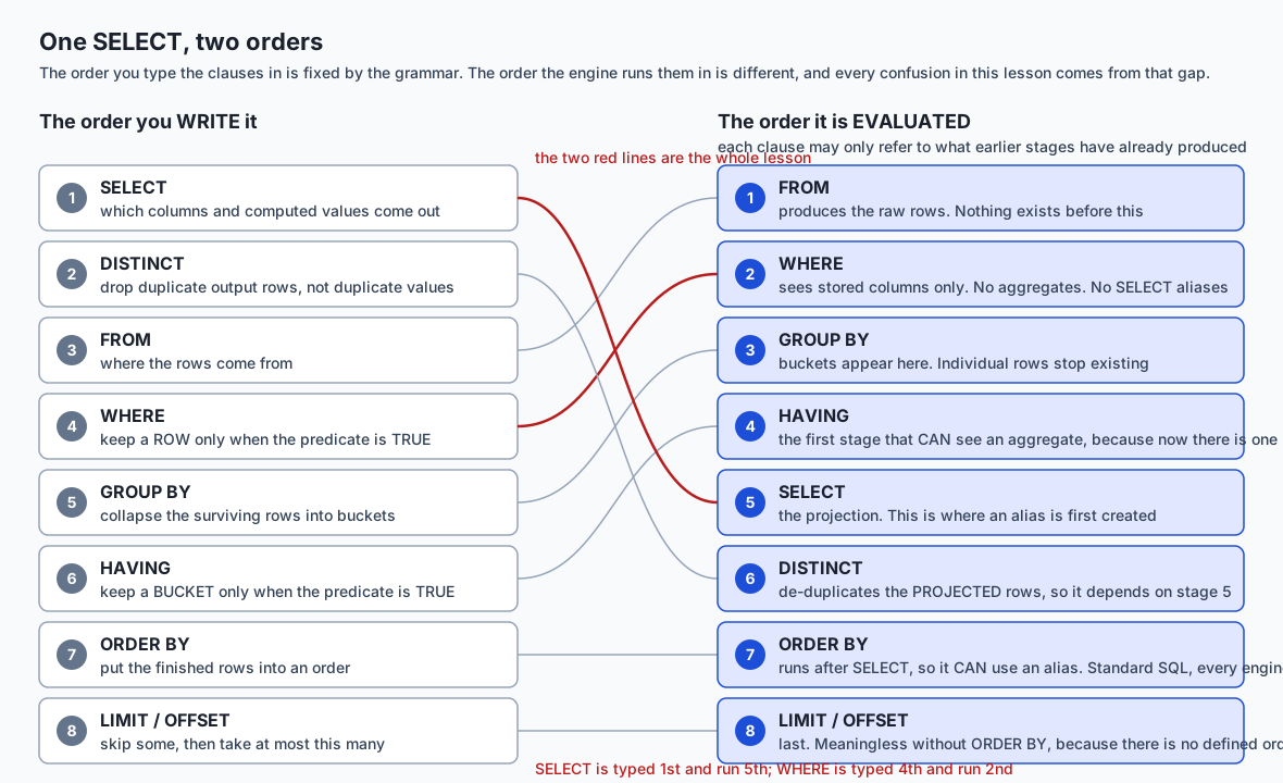
Here is the same thing as a table, because you will come back to it:
| Written | Clause | Evaluated | What it may refer to | What it does to the row count |
|---|---|---|---|---|
| 1st | SELECT | 5th | stored columns, grouping keys, aggregates | never changes it |
| 2nd | DISTINCT | 6th | the projected output rows | can only reduce it |
| 3rd | FROM | 1st | the tables themselves | produces it |
| 4th | WHERE | 2nd | stored columns only | can only reduce it |
| 5th | GROUP BY | 3rd | stored columns and expressions over them | replaces rows with buckets |
| 6th | HAVING | 4th | grouping keys and aggregates | can only reduce the buckets |
| 7th | ORDER BY | 7th | everything, including SELECT aliases | never changes it |
| 8th | LIMIT / OFFSET | 8th | nothing; it just counts | can only reduce it |
Three predictions fall straight out of that table, and you can check all three in the lab.
Why does WHERE COUNT(*) > 3 fail? Because WHERE runs at stage 2 and counts do not exist until stage 3. SQLite says so plainly: Error: in prepare, misuse of aggregate: COUNT().
Why does HAVING exist at all? Because there is no other stage that runs after the buckets are built and before the output is projected. It is not redundant with WHERE; the two filter different objects at different times.
Why can ORDER BY use an alias? Because it runs at stage 7 and aliases are born at stage 5.
Historical background
The relational model was published by Edgar F. Codd, a British mathematician working at IBM’s San Jose laboratory, in “A Relational Model of Data for Large Shared Data Banks”, in Communications of the ACM, June 1970. Codd’s proposal was radical for its time: describe data as sets of tuples with a mathematical foundation, and let the user say what they want rather than how to fetch it. Navigation — the “how” — becomes the machine’s problem.
The language came a few years later. Donald D. Chamberlin and Raymond F. Boyce, also at IBM San Jose, designed SEQUEL (Structured English Query Language) and described it in 1974, as the query language for the experimental System R database. The name was later shortened to SQL because “Sequel” was already a registered trademark of another company, and the pronunciation “sequel” survives to this day among people who learned it in that era.
What matters for today is that GROUP BY and HAVING were in SEQUEL from the start. They are not later bolt-ons. The design intent from the beginning was that a query language should be able to summarise, not merely retrieve, and that summarising needs its own filter because filtering rows and filtering summaries are different operations.
SQL became an ANSI standard in 1986 and an ISO standard in 1987, with the SQL-92 revision being the one most people mean when they say “standard SQL”. The standardisation is the reason the queries you write today mostly move between engines unchanged — and the divergences that remain, several of which you will meet in the lab, are exactly the places where an implementation chose convenience over the standard.
NULL has the most contested history of anything in this lesson, and it is worth knowing that the argument is real rather than assuming everyone agrees. Codd introduced a marker for missing information into the relational model, and with it three-valued logic: a comparison involving a missing value yields neither true nor false but unknown. C. J. Date, one of the most prominent writers on relational theory, argued at length and for decades that NULL was a mistake and that missing information should be handled by other means. Neither side won. NULL is in every mainstream SQL engine, and every mainstream SQL engine’s users trip over it. The traps in this lesson are not implementation bugs; they are the faithful, correct behaviour of a design decision taken fifty years ago that reasonable people still disagree about.
SQLite, the engine you are using, was written by D. Richard Hipp and first released in August 2000. Its distinguishing choice — a library and a single file rather than a server — is why it is on your phone, in your browser and in your operating system, and why today’s lab needs nothing installed.
What it is — and what it is not
A SELECT statement is a description of a result. You state the properties of the rows you want; the engine decides how to find them. That declarative quality is the whole point of the relational model, and it is easy to lose sight of when you are learning the syntax.
It is not a loop. This is the single most useful mental adjustment for someone arriving from Python. You are not iterating over books and testing each one. You are describing a set. The engine may in fact loop, or it may use an index, or it may scan two structures in parallel — that is its business, and it will change its mind when you add an index or when the table grows. Writing SQL as though it were a loop, one row at a time, is how people end up with a program that issues ten thousand queries where one would have done.
It is not a program. A SELECT has no variables, no assignment, no sequence of steps you control. The clause order you are learning today is the engine’s, not yours. You cannot say “first do this, then do that”; you can only describe the shape of the answer.
It does not guarantee an order unless you ask for one. A table is a set of rows, and a set has no order. If your query has no ORDER BY and the rows come back in a pleasing sequence, that is an accident of how the data happens to be stored today. Add an index, insert a row, upgrade the engine, and the accident stops happening. The bug this causes is nasty precisely because it works for months first.
SELECT does not modify anything. It reads. You can run every query in this lesson against a production database and change nothing. That is worth internalising early, because it means the way to understand a database is to ask it, not to guess.
NULL is not a value. It is not zero, not the empty string, not False, not “unknown value” in the sense of an unknown number. It is a marker meaning there is no value here. Two missing things are not equal to each other, because there is nothing to compare. Once you accept that sentence, NULL = NULL returning “unknown” stops being strange and becomes the only defensible answer.
An aggregate is not a scalar function. UPPER(title) takes one row’s value and returns one value: run it over 24 rows and you get 24 answers. COUNT(*) takes many rows and returns one. That difference is why one of them is legal in WHERE and the other is not.
Why it was created and what problems it solves
Before the relational model, asking a database a new question meant writing a program. The data had a physical shape — hierarchies, linked records, explicit pointers between them — and your code walked that shape. Change the shape and every program broke. Ask a question nobody had anticipated and there was no path through the pointers to answer it.
Codd’s proposal solved three problems at once, and all three are still the reason SELECT looks the way it does.
Ad-hoc questions. The whole value of a query language is that you can ask something the schema designer never thought of. “How many books in each genre published since 2000, but only genres with at least three of them” is not a question anybody designs a data structure around. In SQL it is one statement, and today you will write it.
Separating what from how. You say WHERE genre = 'science'. Whether the engine scans every row or jumps straight to an index is a decision it makes, and re-makes, without you rewriting anything. This is why adding an index can make a query a thousand times faster without changing a character of it.
Summarising in the engine, not in your program. This one is easy to underrate until you have felt it. Suppose you want the average rating per genre. Without aggregates you would fetch every row into your program and add them up yourself. That means moving all the data across a process boundary, or a network, to compute six numbers. GROUP BY computes those six numbers where the data already lives and sends you six rows. When the table has twenty-four rows the difference is nothing. When it has two hundred million — the size of a perfectly ordinary training-data index — the difference is the entire feasibility of the question.
HAVING exists for the same family of reasons. “Genres with at least three books” is a fact about a group, and there is no row anywhere that knows how many books its genre has. Without HAVING you would have to compute all the groups, ship them out, and filter them in your own code — which is exactly the “fetch everything and sort it out later” pattern the relational model was invented to end.
How it works
Now walk one real query through all seven stages, with the actual counts from the lab database at every step. The query:
SELECT   genre, COUNT(*) AS n
FROM     books
WHERE    published_year >= 2000
GROUP BY genre
HAVING   COUNT(*) >= 3
ORDER BY COUNT(*) DESC
LIMIT    2;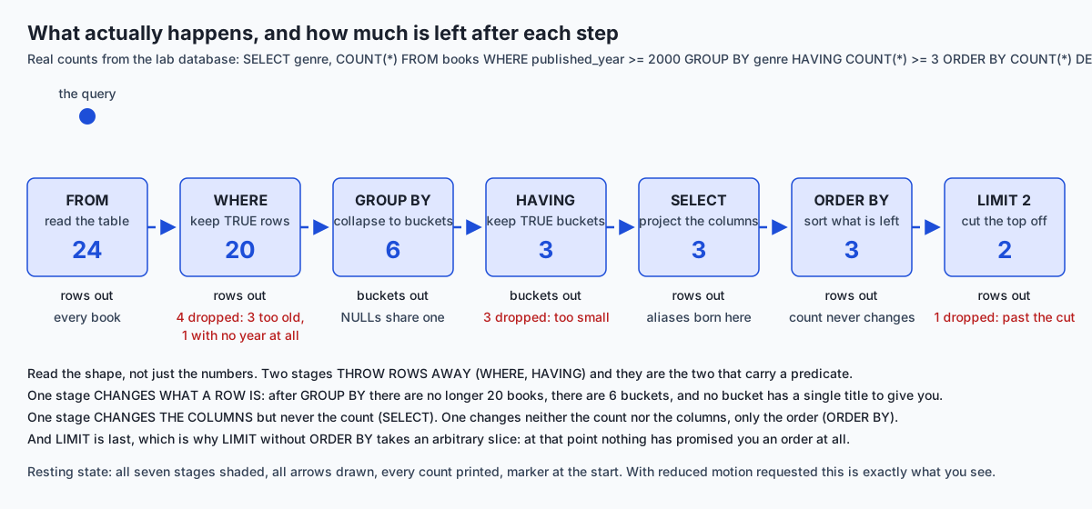
FROM books → 24 rows. Every book in the catalogue.
WHERE published_year >= 2000 → 20 rows. Four disappeared. Three of them were published before 2000, which is what you asked for. The fourth has published_year set to NULL, and it disappeared for a completely different reason that nothing in the query mentions: NULL >= 2000 is unknown, and unknown is not TRUE. That single row is a preview of the entire next section.
GROUP BY genre → 6 buckets. Twenty rows become six buckets: science, fiction, mystery, history, poetry, and one more holding the books whose genre is NULL. Note the surprise: GROUP BY treats all the NULLs as belonging together, which is the one place in SQL where NULLs are grouped as if they were equal. COUNT(DISTINCT genre) on the same table returns 5, because it skips NULLs entirely. Six and five, from the same column, in the same breath.
HAVING COUNT(*) >= 3 → 3 buckets. science has 7, mystery has 4, fiction has 3, and the other three buckets have 2 each and are discarded.
SELECT genre, COUNT(*) AS n → 3 rows, 2 columns. The projection. The alias n comes into existence here and not before.
ORDER BY COUNT(*) DESC → still 3 rows. Sorting never changes the count.
LIMIT 2 → 2 rows. The final result, verified on the authoring machine:
genre    n
-------  -
science  7
mystery  4
Filtering rows: WHERE
WHERE takes a predicate — an expression that evaluates to true, false, or unknown — and keeps the rows where it is true.
The comparison operators are =, <> (also spelled !=), <, <=, >, >=. The boolean operators are AND, OR, NOT. And there is a precedence rule that catches everybody exactly once: AND binds more tightly than OR, just as multiplication binds more tightly than addition. So this:
WHERE genre = 'science' OR genre = 'history' AND published_year >= 2015does not mean what its layout suggests. It means science books of any year, or history books since 2015. In the lab database that matches 8 rows. Put the brackets in:
WHERE (genre = 'science' OR genre = 'history') AND published_year >= 2015and it matches 5. Both queries run. Neither warns you. Write the brackets even when you do not need them.
IN is the readable form of a chain of ORs: genre IN ('poetry', 'mystery') instead of genre = 'poetry' OR genre = 'mystery'. BETWEEN is the readable form of two comparisons, and it is inclusive at both ends: published_year BETWEEN 2015 AND 2018 covers 2015, 2016, 2017 and 2018 — four years, and in the lab, four books. People who assume it is exclusive lose the boundary rows silently.
Matching patterns: LIKE and GLOB
SQLite gives you two pattern matchers, and they differ in ways that will bite you if you treat them as interchangeable.
LIKE | GLOB | |
|---|---|---|
| Any run of characters | % | * |
| Exactly one character | _ | ? |
| Character class | not available | [abc], [A-M] |
| Case sensitivity for ASCII letters | insensitive by default | always sensitive |
| Where it comes from | standard SQL | Unix filename globbing |
The case rule is the one that costs time. In the lab, two titles contain the word “Archive” with a capital A:
SELECT COUNT(*) FROM books WHERE title LIKE '%archive%';   -- 2
SELECT COUNT(*) FROM books WHERE title GLOB '*archive*';   -- 0
SELECT COUNT(*) FROM books WHERE title GLOB '*Archive*';   -- 2
Two, zero, two. The middle query is not broken; it is doing exactly what it was told, and returning nothing is a perfectly ordinary result that you have no reason to question.
Two more things worth knowing. SQLite’s LIKE is case-insensitive only for the 26 ASCII letters — it does not fold case for accented or non-Latin characters unless the engine was built with the optional ICU support. And the _ wildcard is exactly one character: 'The ____ Algorithm' with four underscores matches nothing in the lab, because the word is “Quiet”, which is five letters. Five underscores finds it. Again: no error, just silence.
NULL, and three-valued logic done properly
This is the part of the day to slow down for.
SQL does not have two truth values. It has three: TRUE, FALSE, and UNKNOWN. Any comparison involving NULL produces UNKNOWN, because there is nothing there to compare. And WHERE keeps a row only when the predicate is TRUE — UNKNOWN rows are discarded exactly like false ones, which is why the loss is invisible.
Here is the truth table. Every cell was verified by running it on sqlite3 3.51.0; the shell prints an empty result for UNKNOWN, 1 for true and 0 for false.
A | B | A AND B | A OR B | NOT A |
|---|---|---|---|---|
| TRUE | TRUE | TRUE | TRUE | FALSE |
| TRUE | FALSE | FALSE | TRUE | FALSE |
| TRUE | UNKNOWN | UNKNOWN | TRUE | FALSE |
| FALSE | FALSE | FALSE | FALSE | TRUE |
| FALSE | UNKNOWN | FALSE | UNKNOWN | TRUE |
| UNKNOWN | UNKNOWN | UNKNOWN | UNKNOWN | UNKNOWN |
Read the two bold rows in the middle carefully, because they are where the intuition is genuinely counter-intuitive rather than merely unfamiliar.
NULL AND 0 is FALSE, not unknown. Why? Because it does not matter what the missing value turns out to be: false AND anything is false. The logic can reach a definite answer without knowing the missing operand.
NULL OR 1 is TRUE, for the mirror-image reason: true OR anything is true.
But NULL AND 1 is unknown, and NULL OR 0 is unknown, because in those cases the answer really does depend on the value nobody supplied. Three-valued logic is not arbitrary; it is what you get if you insist that every expression must be correct for every value the missing one could turn out to have.
And NOT NULL is UNKNOWN. The opposite of “I do not know” is “I do not know”. This is why NOT (city = 'Pune') does not rescue you either — negating unknown gives unknown, and the row is still dropped.
The only test for absence is IS NULL (and its partner IS NOT NULL). Uniquely among SQL’s comparisons, it always returns true or false and never unknown. SQLite also lets you write IS and IS NOT between arbitrary expressions as a NULL-safe equality — a IS b is true when both are NULL — which is the same idea other engines spell IS NOT DISTINCT FROM.
Now the three traps, in the order you will meet them.
Trap one: = NULL. Fifteen loans are outstanding. WHERE returned_on = NULL returns 0, because every comparison is unknown. WHERE returned_on IS NULL returns 15.
Trap two: negative filters on a nullable column. WHERE city <> 'Pune' returns 8 out of 12 members, and 2 of those members are in Pune, so 2 people have vanished. If you mean “everyone who is not recorded as being in Pune”, you must say so:
WHERE city IS NULL OR city <> 'Pune'The same trap wears a different hat as NOT IN. WHERE genre NOT IN ('poetry','mystery') returns 14 of the 24 books, not 17, because the three books with a NULL genre are dropped along with the seven that matched.
Trap three: filling the holes. The tempting fix is to make the NULLs go away — COALESCE(rating, 0) and be done with it. But AVG already ignores NULLs, so this does not “handle” the missing ratings; it invents four books rated zero and mixes them into the arithmetic. In the lab:
SELECT ROUND(AVG(rating), 2) FROM books;                  -- 4.16
SELECT ROUND(AVG(COALESCE(rating, 0.0)), 2) FROM books;   -- 3.47
More than half a point of difference, from a change that reads like tidying up. The test suite in the lab has a whole section devoted to keeping that distinction pinned down, because “fixing” the NULLs is the single most common way people make this lesson’s problems appear to go away while making their numbers wrong.
COALESCE(a, b, ...) returns its first non-NULL argument, IFNULL(a, b) is the two-argument version, and NULLIF(a, b) is the inverse — it returns NULL when the two are equal, which is how you turn a sentinel value like 0 or 'unknown' back into an honest absence. All three are legitimate and useful. The rule is to substitute for display, and to think very hard before substituting for arithmetic.
Sorting, and where the NULLs land
ORDER BY takes a list of keys, each optionally ASC (the default) or DESC. The first key decides; later keys only break ties. ORDER BY genre ASC, rating DESC gives you every fiction book before any history book, and within fiction the best-rated first. If you wanted the best book overall you needed the keys the other way round — a distinction that produces two completely different answers from the same two keys, with no error either way.
Where do NULLs sort? SQLite treats NULL as smaller than everything, so ascending puts them first and descending puts them last. That default is the wrong way round for the query people usually want: ORDER BY rating ASC LIMIT 1 returns a book with no rating rather than the worst-rated book. Two fixes, both in the lab:
ORDER BY rating ASC NULLS LAST      -- SQLite 3.30 (2019) and newer
ORDER BY rating IS NULL, rating ASC -- works on every version, and elsewhere
The second is worth understanding rather than copying. rating IS NULL is a predicate, and a predicate evaluates to 0 or 1, so sorting on it ascending puts all the 0s — the rows that have a rating — before all the 1s.
LIMIT n takes the first n rows and OFFSET m skips m first. Two warnings.
LIMIT without ORDER BY is a coin toss, and worse, a coin toss that lands the same way every time until the day it does not. Always pair them, and give the sort a tie-breaker so the result is deterministic when two rows have the same key: ORDER BY rating DESC, title ASC.
And OFFSET gets slow, unavoidably. To give you LIMIT 20 OFFSET 100000 the engine must produce the first 100,000 rows in order and throw them away. The work is proportional to the offset, so page 5,000 costs five thousand times what page 1 cost. It is fine for the first few pages of a user interface and hopeless for walking through a large table. The alternative — keyset pagination — remembers the last key you saw and asks for what comes after it (WHERE id > :last_id ORDER BY id LIMIT 20), which costs the same for every page. You will meet indexes later this week; that is what makes keyset pagination fast.
DISTINCT removes duplicate rows, not duplicate values in a column. SELECT DISTINCT author FROM books gives 7 authors; SELECT DISTINCT author, genre FROM books gives 15 rows, one per distinct pair. Adding a column to a DISTINCT query can only ever increase the number of rows it returns.
Computed columns, aliases, and scalar functions
Anything in the SELECT list can be an expression, and AS names it:
SELECT title, ROUND(pages / 250.0, 2) AS evenings_needed FROM books;Note 250.0 and not 250. Integer division truncates; the decimal point forces real arithmetic. That is a quiet source of zeros in report columns.
The scalar functions worth having at your fingertips: LENGTH, UPPER, LOWER, SUBSTR, REPLACE, TRIM, ABS, ROUND, CAST, TYPEOF, and the date functions DATE, STRFTIME and JULIANDAY. Concatenation is ||, not +. And the rule that ties back to NULL: a scalar function applied to NULL almost always returns NULL. LOWER(genre) on a book with no genre gives NULL, not an empty string, and the NULL then propagates through everything downstream.
SQLite has no date type — dates are TEXT in ISO-8601 form — so date arithmetic must go through the functions. In the lab, loan 2 was borrowed on 2026-01-05 and returned on 2026-02-02:
SELECT JULIANDAY(returned_on) - JULIANDAY(borrowed_on) FROM loans WHERE loan_id = 2;  -- 28.0
SELECT returned_on - borrowed_on              FROM loans WHERE loan_id = 2;           -- 0
The second returns 0 because SQLite coerces each string to the number at its front — 2026 minus 2026. Confident, formatted, and nonsense.
CASE is SQL’s if/elif/else, and it evaluates its branches in order, stopping at the first one that is TRUE:
CASE
  WHEN rating IS NULL THEN 'unrated'
  WHEN rating >= 4.5  THEN 'excellent'
  WHEN rating >= 4.0  THEN 'good'
  ELSE                     'poor'
END
Put the NULL branch anywhere but first and it never fires, because rating >= 4.5 on a NULL is unknown, so every unrated book falls through to the ELSE. In the lab this moves four books out of unrated and into poor, taking the poor band from 6 to 10 — and labelling four books nobody has assessed as the worst in the library.
Aggregates, and what NULL does to each of them
Five aggregates cover most of what you need: COUNT, SUM, AVG, MIN, MAX. SQLite adds TOTAL, which is SUM returning 0.0 instead of NULL over an empty set.
The rule that explains all of their behaviour: every aggregate except COUNT(*) ignores NULL inputs. It does not treat them as zero. They are removed before the arithmetic starts.
| Expression | On the 24 books | What it counts |
|---|---|---|
COUNT(*) | 24 | rows, unconditionally |
COUNT(rating) | 20 | non-NULL values in that column |
COUNT(genre) | 21 | non-NULL values in that column |
COUNT(DISTINCT genre) | 5 | distinct non-NULL values |
AVG(rating) | 4.16 | sum of the 20 values, divided by 20 |
MIN(rating) | 3.2 | smallest non-NULL value |
MAX(rating) | 4.9 | largest non-NULL value |
COUNT(*) versus COUNT(column) is the most useful pair on that list, and it is the cheapest data-quality check in existence. The gap between them is the number of missing values. Get into the habit of putting both in every summary you write:
SELECT COUNT(*) AS rows, COUNT(rating) AS rated, AVG(rating) FROM books;An average that does not say how many values it is based on is an average you cannot act on. AVG(rating) is 4.16 whether it averages twenty ratings or two.
Two edge cases you will meet. SUM over an empty set is NULL, not zero — SQLite’s TOTAL returns 0.0 for the same rows, which is why it exists. And an aggregate over zero rows still returns exactly one row: SELECT COUNT(*), AVG(rating) FROM books WHERE published_year = 1066 gives you one row containing 0 and NULL. That surprises people writing code that expects “no matching rows” to mean “no result”.
Grouping
GROUP BY splits the surviving rows into buckets by a key and runs the aggregates once per bucket.
SELECT   IFNULL(genre, '(unclassified)') AS genre_label,
         COUNT(*)      AS books,
         COUNT(rating) AS rated,
         ROUND(AVG(rating), 3) AS avg_rating
FROM     books
GROUP BY genre
ORDER BY books DESC, genre_label;
Real output from the lab:
genre_label     books  rated  avg_rating
--------------  -----  -----  ----------
science         7      5      4.3
fiction         4      4      3.875
mystery         4      4      4.45
(unclassified)  3      3      4.1
history         3      2      4.05
poetry          3      2      4.0
Look at the science row: 7 books, 5 rated, average 4.3. That average is over five numbers. Without the rated column you would have no way to know, and you would quote 4.3 as “the average rating of science books” when two of the seven have never been rated at all.
You can group by an expression, not just a column, which is how you build histograms:
SELECT (published_year / 10) * 10 AS decade, COUNT(*) AS n
FROM books WHERE published_year IS NOT NULL
GROUP BY decade ORDER BY decade;
Integer division truncates, so 2017 / 10 * 10 is 2010. And you can group by several keys, which gives one row per combination that actually occurs — never a row for a combination with no data. That last point matters when you are producing a summary table for a report: the absent combinations are absent, not zero, and if you need them to appear as zeros you have to arrange it yourself.
HAVING
HAVING filters buckets. The canonical example:
SELECT author, COUNT(*) AS titles
FROM books GROUP BY author
HAVING COUNT(*) > 3
ORDER BY titles DESC, author;
Three authors qualify in the lab, the largest being Ada Fenwick with 5. Try to write the same thing with WHERE and SQLite stops you:
Error: in prepare, misuse of aggregate: COUNT()That error message is the evaluation order made audible. At the moment WHERE runs, there are no groups, so there is nothing for COUNT to count.
WHERE and HAVING are not alternatives and a query commonly wants both, doing different jobs:
SELECT genre, COUNT(*) AS n
FROM books
WHERE published_year >= 2000   -- throws away ROWS
GROUP BY genre
HAVING COUNT(*) >= 2;          -- throws away BUCKETS
When a filter can go in WHERE, put it there. WHERE runs earlier, so it reduces the number of rows that ever have to be grouped. Putting a row-level condition in HAVING usually still gives the right answer and always does more work.
One place SQLite is more permissive than the standard
Two of them, in fact, and you should know both because the code you write today may be run against PostgreSQL next year.
Bare columns in an aggregate query. This runs in SQLite:
SELECT genre, title, COUNT(*) FROM books GROUP BY genre;title is neither a grouping key nor an aggregate, so there is no principled answer — the bucket contains seven titles. SQLite picks one of them, arbitrarily. PostgreSQL rejects the query outright. SQLite documents this leniency and defines the special case where it is meaningful (a bare column alongside MIN or MAX comes from the row that produced that minimum or maximum), but outside that case, treat a bare column as a bug that happens to run.
A SELECT alias used in WHERE. By the evaluation order, this should be impossible: the alias does not exist when WHERE runs. Standard SQL forbids it and PostgreSQL rejects it. SQLite accepts it, verified here on 3.51.0:
$ sqlite3 examples/library.db 'SELECT title, pages*2 AS reading_minutes FROM books WHERE reading_minutes > 800;'
Grammar of Machines|960
Salt and Longitude|1056
The Lost Cartographers|1224
Continental Drift Blues|842
Coasts of Elsewhere|910
The Long Instrument|1024
So the mental model — WHERE runs before SELECT, therefore the alias is not available — is the right model, and it correctly predicts what standard SQL and PostgreSQL do. SQLite is being helpful, and its helpfulness is a portability trap. Repeat the expression, or wrap the query, and it runs everywhere.
An everyday analogy
Picture a reference librarian at a desk, and you hand over a request slip.
The slip is written in the order the form demands: what you want to see at the top, which shelves to look at underneath, then your conditions, then how to group things, then how to sort it, then how much you want.
The librarian does not work in that order. Nobody could. She works like this.
She walks to the shelves and comes back with an armful of books — FROM. Until she has done that, there is nothing to talk about.
She stands at the desk and goes through the pile one book at a time, putting back the ones that do not match your condition — WHERE. She is looking at one book at a time, so she can see anything printed on that book, and nothing else. If your slip said “only books whose genre has more than three titles in it”, she is stuck: she is holding one book, and no book knows how many siblings it has.
She sorts the survivors into piles on the desk, one pile per genre — GROUP BY. And now something has changed that you cannot undo. There are no longer twenty books on the desk; there are six piles. If you now ask her for “the title”, she has no answer — she is looking at a pile of seven.
She looks at the piles and sweeps the small ones off the desk — HAVING. Now the question about pile size is answerable, because now the piles exist. Same librarian, same kind of judgement as before, applied to a different kind of object at a different moment.
She takes a blank sheet and writes down, for each remaining pile, only the things you asked for: the genre, and how many are in it — SELECT. This is the first moment anything gets a name on the sheet.
She crosses out any duplicate lines — DISTINCT — puts the sheet in the order you asked for — ORDER BY — and tears off the top two lines — LIMIT.
The analogy earns its keep because it makes the awkward rules obvious rather than memorable.
Why can ORDER BY use a name that WHERE cannot? Because the name was written on the sheet at the SELECT stage, and WHERE happened while she was still holding books, before any sheet existed.
Why is LIMIT without ORDER BY arbitrary? Because tearing the top off an unsorted sheet gives you whichever lines happened to land there.
And the NULL rule fits too. Suppose a book has no genre printed on it at all. You asked for “not history”. She looks at the spine, finds nothing, and cannot honestly say the book is not history — she does not know what it is. Her instruction is to keep books that definitely match. She puts it back. Nothing on your sheet ever mentions that a book was set aside for lack of information, and this is precisely why the missing rows are invisible: the sheet records what was kept, never what could not be decided.
Examples in practice
Everything below was run for real, in the lab, and the numbers are captured output rather than expectation.
A filter that is honest about missing data. Two versions of “members not from Pune”, against 12 members of whom 2 are in Pune and 2 gave no city:
SELECT COUNT(*) FROM members WHERE city <> 'Pune';                    -- 8
SELECT COUNT(*) FROM members WHERE city IS NULL OR city <> 'Pune';    -- 10
A data-quality check in one line. The gap between the two counts is the number of missing values, and it costs nothing to include:
SELECT COUNT(*) AS books, COUNT(rating) AS rated, COUNT(genre) AS classified FROM books;
-- 24  20  21
A top-N that is deterministic. The sort has a tie-breaker, and NULLs are pushed out of the way rather than winning by accident:
SELECT title, rating FROM books
ORDER BY rating DESC NULLS LAST, title ASC
LIMIT 5;
A histogram, by grouping over a CASE. Real output:
band       n
---------  -
good       8
excellent  6
fair       4
unrated    4
poor       2
Four books are unrated, and they are unrated only because the CASE puts the NULL branch first. Remove that branch and those four are silently reported as poor, taking that band from 2 to 10.
Building GROUP BY from scratch
The clearest way to stop finding aggregates magical is to write one. The lab’s examples/groupby_from_scratch.py implements the whole pipeline in plain Python — no third-party library, just a dictionary of accumulators — and then runs the one-line SQL that replaces it and asserts they agree.
The stages are four small functions. WHERE, in Python, makes the three-valued logic explicit in a way SQL never does:
def where(rows):
    """WHERE published_year >= 2000 — rows with a NULL year cannot qualify."""
    kept = []
    for row in rows:
        year = row["published_year"]
        if year is None:
            continue          # UNKNOWN, and UNKNOWN is not TRUE
        if year >= 2000:
            kept.append(row)
    return kept
That if year is None: continue is the entire mystery of the disappearing rows, written out. SQL does the same thing; it just does not show you the line.
Then GROUP BY is a dictionary keyed by the grouping value, where None is a perfectly good key — which is exactly why all the NULLs land in one bucket:
for row in rows:
    key = row["genre"]                 # None is a real key, not an error
    acc = buckets.setdefault(key, new_accumulator())
    acc["rows"] += 1                   # COUNT(*) counts the ROW
    rating = row["rating"]
    if rating is not None:             # every other aggregate SKIPS NULL
        acc["rating_n"] += 1
        acc["rating_sum"] += rating
Look at what you were forced to decide. acc["rows"] += 1 happens unconditionally — that is COUNT(*). The rating accumulator is guarded by if rating is not None — that is every other aggregate. There was never a sensible alternative: you cannot add None to a running total. “AVG ignores NULLs” is not a rule somebody imposed; it is the only thing that could have happened.
Twenty lines of Python, and this is what replaces them:
SELECT   IFNULL(genre, '(unclassified)') AS genre_label,
         COUNT(*) AS books, COUNT(rating) AS rated,
         ROUND(AVG(rating), 6) AS avg_rating,
         MIN(rating) AS min_rating, MAX(rating) AS max_rating,
         ROUND(AVG(pages), 6) AS avg_pages
FROM     books
WHERE    published_year >= 2000
GROUP BY genre
HAVING   COUNT(*) >= 3
ORDER BY books DESC, genre_label ASC
Running the script prints both tables and compares them row by row. The real output ends:
The 20 lines of Python:
  FROM      -> 24 rows
  WHERE     -> 20 rows survive
  GROUP BY  -> 6 buckets
  HAVING    -> 3 buckets survive

genre_label  books  rated  avg_rating  min_rating  max_rating  avg_pages
-----------  -----  -----  ----------  ----------  ----------  ----------
science      7      5      4.3         3.7         4.8         326.285714
mystery      4      4      4.45        4.3         4.6         292.5
fiction      3      3      4.1         3.5         4.7         443.666667

IDENTICAL: 3 rows match exactly.
Two things to take from that. The SQL is shorter, and that is the least interesting of its advantages: the important one is that the SQL runs where the data is, so it scales to a table that would never fit in your program’s memory. And the Python is not wasted effort — it is the reason you now know precisely what the engine is doing, which is what you need when a query is slow or a number looks wrong.
Implications: security, privacy, performance, scalability, and cost
Security. Every query in this lesson is a fixed string. The moment you build one by pasting a value in, you have created the most common serious vulnerability in application software. Never do this:
cur.execute("SELECT * FROM books WHERE author = '" + name + "'")If name is x' OR '1'='1, the query returns the whole table. The fix is not to escape the quotes yourself — thirty years of people getting that wrong says otherwise. The fix is to never build the string:
cur.execute("SELECT * FROM books WHERE author = ?", (name,))Python’s sqlite3 module sends the query text and the values along separate paths, so no value can change the shape of the statement no matter what characters it contains. Also worth saying plainly: a WHERE clause is not access control. It filters what one query returns; it does nothing to stop the same connection running a different query without it.
Privacy, and it belongs to today specifically. Aggregation is routinely offered as a privacy measure — “we only publish counts, never individual records”. Be careful with that claim. A GROUP BY whose buckets are small anonymises nothing: a count of 1 identifies exactly one person, and two published aggregates that differ by one row tell you what that row contained. The habit to form now, while the stakes are a fictional library, is to look at the smallest bucket in any grouped result before publishing it. When you are reporting model performance by demographic slice later in this course, that habit is the difference between a responsible evaluation and an accidental disclosure.
Performance. Four things dominate, and all four are consequences of the evaluation order.
Filter early. A condition in WHERE reduces the rows that ever reach GROUP BY. The same condition in HAVING often gives the same answer after doing far more work.
WHERE on a bare column can use an index; WHERE on a function of that column usually cannot. WHERE published_year >= 2000 can jump straight to the right part of an index. WHERE (published_year / 10) * 10 >= 2000 must compute the expression for every row first. Same rows, completely different cost, and nothing about the query text tells you which you wrote.
ORDER BY may need to materialise and sort everything. If there is no index in the sort order, the engine must gather all the qualifying rows before it can return the first one — so a query with LIMIT 10 can still read the entire table.
OFFSET is linear in the offset. Discussed above: it is fine for page 2 and disastrous for page 5,000.
Scalability. The reason GROUP BY matters so much for the rest of this course is that it moves the computation to the data. Six numbers come back instead of two hundred million rows. When your training-data index outgrows your laptop’s memory — and it will — that is not an optimisation, it is the difference between a question you can ask and one you cannot.
Cost. SQLite is free and runs on the machine you already own; today’s lab costs nothing at all. Where money enters is managed databases and cloud warehouses, and there the shape of your query is the shape of your bill: several of them charge by bytes scanned, so a SELECT * where you needed two columns, or a missing WHERE, is billed directly. Pricing changes constantly and varies by region, so read the provider’s current pricing page rather than trusting any figure printed in a course.
Alternatives: free, open source, and commercial
The queries you wrote today are, with the two clearly-marked SQLite exceptions, standard SQL. Here is the honest landscape of where else you could run them, and when you should.
SQLite — free, public domain, already installed. Not merely open source: Hipp placed it in the public domain, which is why it ships inside browsers, phones and operating systems without anyone negotiating a licence. Choose it when the database is used by one machine, one application, or one person: local tools, test fixtures, application data on a device, and every analysis you do on a file you can fit on your disk. How to use it: sqlite3 mydata.db, and it is a file. Concrete example: the entire lab today, 24 books and 45 loans, with nothing installed and nothing to uninstall. Limitation to be honest about: one writer at a time. Many readers are fine; concurrent writers are not what it is for.
PostgreSQL — free and open source, under the PostgreSQL Licence. The reference implementation for people who care about standards compliance. Choose it when several programs or people write at once, when you need real user accounts and permissions, or when you want features SQLite does not have — strict typing, rich date and interval types, window functions over large data, and full-text search. How to use it: run the server (a package on any Linux distribution, or a container), then psql mydb. Concrete example: today’s grouping query runs unchanged:
SELECT genre, COUNT(*) AS n FROM books
WHERE published_year >= 2000 GROUP BY genre HAVING COUNT(*) >= 3;
What differs: PostgreSQL rejects the two SQLite leniencies you met — a bare column in an aggregate query, and a SELECT alias used in WHERE. It also defaults NULLs last on ascending sorts, the opposite of SQLite, so any query that relies on NULL placement without saying NULLS FIRST or NULLS LAST explicitly will silently reorder when you port it. Free to run yourself; every cloud provider sells a managed version, priced per hour and per gigabyte.
MySQL and MariaDB — free and open source, the other default for web applications. Choose it when you are working with an existing stack that already uses it. What differs: LIKE is case-insensitive or not depending on the column’s collation rather than on the operator, which is a genuinely different model from SQLite’s and a common source of surprise when porting either way. MySQL is offered under a dual licence by Oracle; MariaDB is the community fork.
DuckDB — free, open source (MIT), and the most interesting recent arrival for anyone doing data work. It is SQLite’s shape — a library, an embedded file, nothing to run — but column-oriented, which makes it dramatically faster at exactly the queries this lesson is about: scanning many rows to compute a few aggregates. Choose it when you are aggregating over millions of rows on one machine, or when you want to query CSV and Parquet files directly without loading them anywhere first. How to use it: duckdb mydata.db, and the SQL is largely the same. Concrete example of what it adds: it will query a file in place — SELECT genre, COUNT(*) FROM 'books.parquet' GROUP BY genre — which for a dataset audit is a genuinely different workflow from “import it first”. Honest caveat: it is for analysis, not for being an application’s transactional store, and I have not run it on this machine, so the syntax above is from its documentation rather than from a capture.
The Python standard library, no database at all. You have already seen it: examples/groupby_from_scratch.py does grouping and five aggregates with dict and a loop. Choose it when the data is small, already in memory, and the logic is more naturally expressed in code than in SQL. Concrete example: the twenty lines in this lesson. Where it stops: every row must fit in memory, you must write and test the aggregation yourself, and you get no index — so a filter is always a full scan. collections.Counter and itertools.groupby shorten it (note that itertools.groupby requires the input to be sorted by the key first, which trips people up), but they do not change the trade-off.
pandas — free and open source (BSD), the dataframe answer to the same questions, and the one most people in this field reach for. Choose it when the data fits in memory, you want to interleave querying with plotting and modelling, and the analysis is exploratory rather than a fixed report. The vocabulary maps closely onto today’s: df[df.published_year >= 2000] is WHERE, .groupby('genre') is GROUP BY, .agg(...) is the aggregate list, .sort_values(...) is ORDER BY, .head(2) is LIMIT. Honest statement: pandas is not installed in this lab and no pandas output is shown anywhere in this lesson, because this week deliberately uses nothing outside the standard library. You will use it properly later. Two things to carry forward when you do: its default for missing data differs from SQL’s in ways that matter (groupby drops NULL keys by default, where SQL gives them their own bucket), and everything must fit in memory, which is the constraint SQL exists to escape.
Commercial and managed services — Amazon RDS and Aurora, Google Cloud SQL and BigQuery, Azure SQL Database, Snowflake, Databricks, Oracle Database, Microsoft SQL Server. Choose them when somebody else running the server is worth paying for, or when the data is genuinely too large for one machine. All of them speak SQL, and most of today’s queries would run on all of them. Several bill by data scanned rather than by time, which makes query shape a direct cost. Prices change frequently and vary by region and commitment; check the provider’s current pricing page rather than any number in a course.
The summary judgement: learn the SQL, not the engine. The clause evaluation order, the three-valued logic and the aggregate rules are the same everywhere. The differences are at the edges, and the edges are documented.
Comparison with related concepts
WHERE versus HAVING. WHERE filters rows before grouping; HAVING filters groups after. WHERE cannot see an aggregate because none exists yet. When a condition could go in either, put it in WHERE — it runs earlier and reduces the work.
COUNT(*) versus COUNT(column) versus COUNT(DISTINCT column). Rows, non-NULL values, distinct non-NULL values. On the lab’s books: 24, 20, and 5 for genre. Three different questions that look almost identical on the page.
GROUP BY versus DISTINCT. SELECT DISTINCT genre FROM books and SELECT genre FROM books GROUP BY genre return the same six rows here. They are not the same tool: GROUP BY can compute aggregates per bucket, DISTINCT only removes duplicates. Use DISTINCT when you want unique rows and GROUP BY when you want a summary — and note that the “same six rows” includes the NULL bucket in both cases, which COUNT(DISTINCT genre) would not.
LIKE versus GLOB versus a regular expression. LIKE is standard SQL and case-insensitive for ASCII; GLOB is Unix-style, case-sensitive, and has character classes. Neither is a regular expression — SQLite’s REGEXP operator has no built-in implementation and only works if the application supplies one. Full-text search is a different mechanism again, built on an index; pattern matching with a leading % cannot use an ordinary index at all, which is why a “search” built out of LIKE '%term%' gets slow as soon as it is useful.
IS NULL versus = NULL versus IS NOT DISTINCT FROM. IS NULL is the test for absence and always returns true or false. = NULL is always unknown and therefore always useless. IS NOT DISTINCT FROM — spelled IS in SQLite — is NULL-safe equality: two NULLs compare equal, which is occasionally exactly what you want when comparing two nullable columns.
Aggregate functions versus window functions. An aggregate collapses many rows into one. A window function computes a value across a set of rows while keeping every row — a running total, a rank within a group, “this row’s value minus the group average”. They use the same functions with an OVER (...) clause. Window functions arrived in SQLite in 3.25 (2018); they are beyond today, and the reason to know they exist is that the query you eventually want — “each book alongside its genre’s average” — needs one, and forcing it out of GROUP BY alone is painful.
Three-valued logic versus Python’s None. Python’s None == None is True; SQL’s NULL = NULL is unknown. Python has two truth values, SQL has three. Both are internally consistent, and translating between them without noticing the switch is a reliable source of bugs — especially in code that builds a filter in Python and hands it to SQL.
Ordering: SQLite versus everything else. SQLite sorts NULLs first ascending. PostgreSQL sorts them last. The standard leaves it implementation-defined. Any query whose correctness depends on where NULLs land should say NULLS FIRST or NULLS LAST out loud, or use ORDER BY col IS NULL, col.
When to use it — and when not to
Use WHERE and GROUP BY in the database when the data is already there, when there is more of it than you want to move, and when the question is a summary. That is most of the time, and it is nearly always the right default. One GROUP BY over two hundred million rows returning six is a question you can ask; the same work in your program is not.
Use HAVING when the condition is about a group. If you find yourself computing an aggregate, fetching the result, and filtering it in Python, you wanted HAVING.
Use a LIMIT with an ORDER BY when you want a top-N. Use keyset pagination instead of OFFSET when you are walking through a large table rather than showing page 2 of a list.
Do not use SQL when the logic is genuinely procedural — multi-step transformations with branching, or anything you would need a debugger for. A CASE inside a CASE inside a subquery is a sign that the logic wants to be in a program. SQL is a language for describing sets; it is a poor language for describing algorithms, and pushing it past that point produces code nobody can maintain.
Do not use SQL when you need something it has no notion of — training a model, calling an API, drawing a chart. Pull the summarised rows out and do that work where it belongs. The point of a good GROUP BY is that what you pull out is small.
Do not use SELECT * in anything you keep. It scans and returns columns you do not need, it breaks silently when somebody adds a column, and in warehouses that bill by bytes scanned it costs money on every run. It is a fine keystroke saver while exploring, and a liability in a file.
Do not trust an aggregate that does not report its denominator. Every summary you write should say how many rows went into it and how many of them had a value. COUNT(*) and COUNT(column) side by side, always. This is the single habit from today that will save you the most.
Do not “fix” NULLs by filling them in until you have decided what the missing value means. Sometimes zero is right — an unrecorded number of sales probably was zero sales. Often it is badly wrong — an unrecorded rating is not a rating of zero, and turning it into one moved this lab’s average from 4.16 to 3.47 without a word of warning. Decide deliberately, write down the decision, and keep the raw column.
The AI thread
Come back to where this started, because now the claim can be made precisely rather than as a slogan.
Every dataset card you will ever write is a page of GROUP BY results. Number of examples per class, per language, per source, per licence, per year of collection. Every one of those is a grouping key and a count. Class imbalance — the thing that quietly ruins a classifier — is literally the output of SELECT label, COUNT(*) FROM examples GROUP BY label ORDER BY 2 DESC, and you find it by looking, or you do not find it.
Every evaluation you run is a filter and an aggregate. Overall accuracy is one aggregate. Accuracy by slice — which is where the real information is, because a model that is 94% accurate overall and 61% accurate on one subgroup is not a 94% model — is GROUP BY slice. And the honest version of that report carries COUNT(*) next to every accuracy figure, because 61% over eleven examples and 61% over eleven thousand are different findings, and HAVING COUNT(*) >= 100 is how you stop yourself drawing conclusions from a bucket of four.
Every data-quality audit is COUNT(*) - COUNT(column). How many rows are missing a label, a licence, a source URL, a language tag. The gap between those two counts is your missing-data report, and it takes ten seconds to write.
And the NULL traps are not an academic curiosity here; they are how datasets get quietly corrupted. WHERE license <> 'restricted' drops every row whose licence was never recorded — the rows you should be most worried about — and hands you a clean-looking dataset. AVG(toxicity_score) over a column where the scorer failed on 8% of rows silently reports the average of the 92% it managed. COALESCE(score, 0) on that column reports something worse: a number that is confidently wrong, computed from data that was never collected.
The through-line for the rest of this course is simple. You cannot curate what you cannot count, you cannot count without filtering first, and you cannot trust either unless you know exactly which rows your filter threw away and why. That is what today was about.
Knowledge check
Answer these from memory before you check them against the lab.
- Write out the eight clauses in the order the engine evaluates them.
- Why is
WHERE COUNT(*) > 3an error, in terms of that order? What is the exact message SQLite gives? - A table has 12 rows, 2 of which have
city = 'Pune'.SELECT COUNT(*) FROM t WHERE city <> 'Pune'returns 8. Explain the missing 2, and write the query that returns 10. - What are
NULL AND 0,NULL AND 1,NULL OR 1,NULL OR 0andNOT NULL? Justify each without memorising it. COUNT(*)is 24 andCOUNT(rating)is 20. What does the difference tell you, and why isAVG(rating)not affected by it?- Why can
ORDER BYuse aSELECTalias? Why does the same query using that alias inWHERErun on SQLite and fail on PostgreSQL? - Where do NULLs sort in SQLite, ascending and descending? Write two ways to force them last.
- Why does
LIMIT 20 OFFSET 100000get slower as the offset grows, and what do you use instead?
Hands-on exercise
Run the lab: labs/sections/programming-with-python/day-086-select-filtering-sorting-and-aggregating/.
Work from the lab README, in this order.
- Build the database:
bash examples/build_db.sh. It printsseeded: 24 books, 12 members, 45 loans. - Read and run the eight query files in
examples/queries/in order, one at a time. Read each file before you run it and predict the answer; every query has a comment saying what it is meant to show. - Run
python3 examples/groupby_from_scratch.pyand read the source alongside the output. Find theif rating is not None:line and satisfy yourself that no other behaviour was available. - Score the twelve exercises before you start:
bash starter/check.sh. All twelve are wrong, and all twelve ran without an error. - Fix them one at a time in
starter/exercises.sql, re-scoring as you go. - Only when
check.shis green, readexamples/exercise-answers.sqlfor the explanation of each. - Run the full suite:
bash tests/run_tests.sh.
Expected output
The suite ends with this, captured from a real run:
14. The lab stays offline, stays out of your way, and cleans up
  ok: no URL anywhere in examples/, starter/ or tests/
  ok: nothing under examples/ or starter/ calls sudo
  ok: no stray database in the lab root
  ok: the built database is git-ignored, so it is never committed

124 checks, 0 failure(s).
And the untouched starter scores like this:
ex01       0                          15                         WRONG
ex02       8                          10                         WRONG
ex03       0                          2                          WRONG
ex04       2                          4                          WRONG
ex05       3.47                       4.16                       WRONG
ex06       20                         4                          WRONG
Validate your work
bash tests/run_tests.shprints124 checks, 0 failure(s).and exits 0.bash starter/check.shprints12 correct, 0 still wrong.and exits 0.python3 examples/groupby_from_scratch.pyprintsIDENTICAL: 3 rows match exactly.and exits 0.SELECT COUNT(*) FROM loans WHERE returned_on IS NULLreturns 15, and the= NULLversion returns 0 without erroring.SELECT ROUND(AVG(rating),2) FROM booksreturns 4.16, and theCOALESCE(rating,0.0)version returns 3.47.SELECT author FROM books WHERE COUNT(*) > 3 GROUP BY authoris rejected withError: in prepare, misuse of aggregate: COUNT().- Break one on purpose: change your fixed exercise 1 back to
= NULLand confirmcheck.shgoes red and exits non-zero. A scorer you have never seen fail is a scorer you have no reason to trust.
Troubleshooting
sqlite3: command not found— macOS ships it; on Debian and Ubuntu the shell is a separate package from the library, sosudo apt install sqlite3.Error: unable to open database file— you are not in the lab directory, or the database is not built.cdto the lab and runbash examples/build_db.sh.Error: no such table: books— you typed a database name SQLite has never seen, and it created a new empty file rather than failing. Delete the stray.dband rebuild.- A query returns 0 rows and you are sure it should not — in this lab that is almost always a NULL. Check for
=or<>against a nullable column, or a negative filter, orNOT IN. misuse of aggregate: COUNT()— an aggregate inWHERE. It belongs inHAVING.ORDER BY ... NULLS LASTis rejected — your SQLite predates 3.30. UseORDER BY rating IS NULL, rating ASC, which works everywhere.
Full details in the lab’s troubleshooting.md.
Common mistakes
- Comparing to NULL with
=or<>. Always unknown, always drops the row.IS NULLis the only test. - A negative filter on a nullable column.
city <> 'Pune'andgenre NOT IN (...)both silently discard the rows where the column is NULL. - Assuming
BETWEENis exclusive. It includes both endpoints. - Forgetting that
ANDbinds tighter thanOR. Two readings of the same words, 5 rows and 8 rows, no warning. - Reaching for
GLOBwhen you wanted case-insensitive matching. OrLIKEwhen you wanted case-sensitive. Zero results is not an error. - Putting the NULL branch of a
CASEanywhere but first. It never fires, and the NULL rows are labelled with whatever theELSEsays. LIMITwithoutORDER BY. An arbitrary slice that happens to look stable until it does not.- Quoting an average without its denominator. 4.16 over twenty ratings and 4.16 over two are different facts.
- “Fixing” NULLs with
COALESCE(col, 0)before deciding what the absence means. It does not handle the missing data; it invents data. - Relying on SQLite’s leniencies. A bare column in an aggregate query, and a
SELECTalias inWHERE, both run here and both fail on PostgreSQL.
Practice assignment
Extend the lab’s database and write the queries that audit it — the same job you will be doing on training data for the rest of this course.
- Add a
reviewstable to your own copy ofexamples/seed.sql:review_id,book_id,member_id,stars(1 to 5, and deliberately nullable), andsubmitted_on. Insert about thirty rows, and make sure at least six have a NULLstars— a review with text but no score. - Write a data-quality report over your new table as a single query: total rows, rows with a score, and the percentage scored. Compute the percentage correctly, which means remembering that integer division truncates.
- Write the review histogram: how many reviews at each star level, with the unscored ones appearing as their own labelled bucket rather than vanishing.
- Write “books with at least three reviews, ordered by average score”, and make the result deterministic — a tie-breaker in the
ORDER BYand an explicit decision about where the unscored reviews go. - Write the same query twice: once treating NULL scores as excluded, once treating them as 3 stars. Print both numbers side by side and write two sentences on which one you would publish and why.
- Find the smallest bucket in any grouping you have produced. Write two sentences on whether that result would be safe to publish if these were real members.
- Add five checks to a copy of
tests/run_tests.shthat pin the actual values your queries return. Then break your seed data on purpose and confirm the checks go red.
Deliverable: your seed.sql additions, a reviews.sql file with the queries and a comment above each saying what it answers, and your captured output.
Extension challenge
- Write the same aggregation three ways — in SQL, in plain Python with a dictionary of accumulators, and using
collections.Counter— and compare them on correctness, length and readability. Then write down what would change if the table had fifty million rows. - Build a subquery. Find every book rated above the overall average. You need the average before you can compare against it, so it goes in an inner query:
WHERE rating > (SELECT AVG(rating) FROM books). Then work out how many rows have to be read, and why the answer is not obvious. - Meet window functions early. Write a query returning every book with its genre’s average rating alongside it, using
AVG(rating) OVER (PARTITION BY genre). Then try to get the same result withGROUP BYalone and note where it becomes painful — that is the boundary that made window functions necessary. - Port it deliberately. Take
examples/queries/06-group-by.sqland mark every statement that would need changing for PostgreSQL. There are two, and both are flagged in the files. Then decide whether you will keep writing the SQLite-only spelling. - Measure
OFFSET. Generate a table of a million rows with a recursiveWITHclause, then timeLIMIT 10 OFFSET 10,OFFSET 100000andOFFSET 900000. Predict the shape of the curve first, then check whether you were right. - Audit something real. Take any CSV you actually have, load it into a SQLite table, and answer three questions about it: how many rows, how many are missing each field, and what the distribution of the most important column looks like. That sequence — count, count the holes, then group — is the first thing to do to any dataset you are handed, and you now know how to do all three.
Quiz
Q1. In what order does a SQL engine logically evaluate the clauses of a SELECT statement?
- SELECT, FROM, WHERE, GROUP BY, HAVING, ORDER BY, LIMIT — the order you type them
- FROM, WHERE, GROUP BY, HAVING, SELECT, DISTINCT, ORDER BY, LIMIT
- FROM, SELECT, WHERE, GROUP BY, ORDER BY, HAVING, LIMIT
- WHERE, FROM, GROUP BY, SELECT, HAVING, DISTINCT, LIMIT, ORDER BY
Show answer
Answer: B. FROM, WHERE, GROUP BY, HAVING, SELECT, DISTINCT, ORDER BY, LIMIT
The rows have to exist before anything can filter them, so FROM is first. WHERE filters individual rows, then GROUP BY replaces those rows with buckets, then HAVING filters the buckets — which is why HAVING is the first stage that can see an aggregate, because it is the first that runs after there is anything to aggregate. SELECT comes fifth, which is the fact that surprises people: it is written first and run fifth, and that inversion explains why an alias invented in SELECT is unavailable to WHERE but available to ORDER BY. DISTINCT operates on what SELECT projected, ORDER BY sorts the finished rows, and LIMIT takes a slice last of all — which is exactly why LIMIT without ORDER BY returns an arbitrary slice.
Q2. A members table has 12 rows. Two of them have city = 'Pune' and two have city set to NULL. What does SELECT COUNT(*) FROM members WHERE city <> 'Pune' return?
- 10, because 12 minus the 2 in Pune is 10
- 12, because <> matches everything that is not exactly the string Pune
- 8, because the two rows with a NULL city evaluate to UNKNOWN and are discarded along with the two from Pune
- An error, because you cannot compare a NULL column with <>
Show answer
Answer: C. 8, because the two rows with a NULL city evaluate to UNKNOWN and are discarded along with the two from Pune
This is the most expensive habit in SQL and it never raises an error. NULL <> 'Pune' is UNKNOWN, not TRUE, and WHERE keeps only rows where the predicate is TRUE — so UNKNOWN rows are discarded exactly like false ones. Two members from Pune are correctly excluded and two members who simply never told the library their city are silently excluded too, leaving 8. The number is plausible, nothing warns you, and if the column were license rather than city and the table were training data, you would have just dropped the rows you most needed to look at. The honest query is WHERE city IS NULL OR city <> 'Pune', which returns 10.
Q3. Which of these is FALSE rather than UNKNOWN?
- NULL AND 0
- NULL AND 1
- NULL OR 0
- NOT NULL
Show answer
Answer: A. NULL AND 0
Three-valued logic is not arbitrary: an expression gets a definite answer whenever that answer would be the same for every value the missing operand could turn out to have. FALSE AND anything is FALSE, so NULL AND 0 is FALSE without needing to know the missing value. By the mirror argument NULL OR 1 is TRUE. But NULL AND 1 depends entirely on the unknown operand, so it is UNKNOWN; NULL OR 0 likewise; and NOT NULL is UNKNOWN because the opposite of "I do not know" is still "I do not know". That last one is why negating a comparison does not rescue you from the trap in the previous question.
Q4. Why is SELECT author, COUNT(*) FROM books WHERE COUNT(*) > 3 GROUP BY author rejected with "misuse of aggregate: COUNT()"?
- COUNT(*) may only appear in the SELECT list, never in a filter
- The GROUP BY has to be written before the WHERE for the count to be in scope
- WHERE runs at stage 2 and the groups do not exist until stage 3, so there is nothing for COUNT to count yet
- COUNT(*) needs a column argument when it is used as a condition
Show answer
Answer: C. WHERE runs at stage 2 and the groups do not exist until stage 3, so there is nothing for COUNT to count yet
The error is the evaluation order made audible. WHERE filters individual rows, and it runs before GROUP BY has built any buckets, so at that moment there is no group whose size COUNT(*) could report — no single row knows how many titles its author wrote. The clause that filters groups is HAVING, which runs at stage 4, after the buckets exist: HAVING COUNT(*) > 3. This is also why HAVING is not redundant with WHERE. They are not two ways of writing the same filter; they filter different kinds of object at different moments, and when a condition genuinely is about a single row you should put it in WHERE, because filtering earlier means fewer rows ever have to be grouped.
Q5. A books table has 24 rows; 4 of them have a NULL rating. What do COUNT(*), COUNT(rating) and AVG(rating) report?
- 24, 24 and the average of all 24 values with the NULLs counted as zero
- 24, 20, and the sum of the 20 real ratings divided by 20 — the NULLs are removed before the arithmetic
- 20, 20, and an average over 20, because rows with any NULL are excluded from the whole query
- 24, 20, and NULL, because an aggregate over a column containing any NULL is undefined
Show answer
Answer: B. 24, 20, and the sum of the 20 real ratings divided by 20 — the NULLs are removed before the arithmetic
COUNT(*) counts rows unconditionally; every other aggregate — COUNT(column), SUM, AVG, MIN, MAX — removes the NULLs before it starts. So AVG divides by the non-NULL count, not by the row count, and in the lab database that is 4.16 rather than the 3.47 you get from AVG(COALESCE(rating, 0.0)). The gap between COUNT(*) and COUNT(column) is the cheapest data-quality check that exists: it IS the number of missing values. Put both in every summary you write, because an average that does not say how many values it is based on is an average you cannot act on — 4.16 over twenty ratings and 4.16 over two are very different findings.
Q6. Your query ends ORDER BY rating ASC LIMIT 1 and you expect the worst-rated book. In SQLite you get a book with no rating at all. Which fix is portable to any SQL engine and any version?
- ORDER BY rating ASC NULLS LAST
- ORDER BY COALESCE(rating, 999) ASC
- ORDER BY rating IS NULL, rating ASC
- Add DISTINCT, which removes the NULL row from the projection
Show answer
Answer: C. ORDER BY rating IS NULL, rating ASC
SQLite sorts NULL as smaller than everything, so ascending puts the unrated books first — and a NULL is not a low rating, it is no rating. rating IS NULL is a predicate that evaluates to 0 for rows that have a value and 1 for rows that do not, so sorting on it ascending pushes all the missing ones to the end, on every engine and every version. NULLS LAST is cleaner to read but arrived in SQLite 3.30 and its placement default differs between engines — PostgreSQL already sorts NULLs last ascending, the opposite of SQLite — so any query whose correctness depends on where NULLs land should say so explicitly. COALESCE to a sentinel works but corrupts the value if 999 is ever a real rating, and DISTINCT does not remove NULL rows at all.
Q7. Which statement about LIKE and GLOB in SQLite is correct?
- Both use % and _ as wildcards; GLOB simply adds character classes
- GLOB is case-insensitive and LIKE is case-sensitive, which is the opposite of most engines
- They are aliases for the same operator and differ only in which one the query planner prefers
- LIKE is case-insensitive for ASCII letters and uses % and _; GLOB is always case-sensitive and uses * and ?
Show answer
Answer: D. LIKE is case-insensitive for ASCII letters and uses % and _; GLOB is always case-sensitive and uses * and ?
LIKE comes from standard SQL, uses % for any run of characters and _ for exactly one, and in SQLite folds case for the 26 ASCII letters by default — but not for accented or non-Latin characters unless the build includes ICU. GLOB comes from Unix filename matching, uses * and ?, adds character classes such as A-M which LIKE has no equivalent for, and is always case-sensitive. In the lab, LIKE '%archive%' finds 2 titles and GLOB '*archive*' finds 0, and the second is not an error — it is a perfectly ordinary empty result that you have no particular reason to question. That silence is the whole hazard.
Q8. You are reporting model accuracy per demographic slice. Which query shape is the responsible one?
- GROUP BY slice with AVG(correct), and publish every slice with its figure
- GROUP BY slice with AVG(correct) and COUNT(*) reported alongside, plus a deliberate look at the smallest bucket before publishing
- WHERE correct = 1 GROUP BY slice, so only the successful predictions are summarised
- AVG(correct) with no GROUP BY, since the overall figure already accounts for every slice
Show answer
Answer: B. GROUP BY slice with AVG(correct) and COUNT(*) reported alongside, plus a deliberate look at the smallest bucket before publishing
Two failures are being guarded against at once. The first is statistical: 61 percent over eleven examples and 61 percent over eleven thousand are different findings, so an accuracy without its denominator cannot be acted on — report COUNT(*) beside every aggregate, and consider HAVING COUNT(*) >= some floor before drawing conclusions. The second is disclosure: aggregation is routinely offered as a privacy measure, but a GROUP BY whose buckets are small anonymises nothing, since a count of one identifies exactly one person and two published aggregates differing by one row reveal what that row contained. Filtering to correct = 1 first is simply the wrong question — it throws away the denominator entirely — and an overall average hides precisely the per-slice gap that makes the report worth writing.
Glossary
- Predicate
- An expression that evaluates to TRUE, FALSE or UNKNOWN — the thing a WHERE or HAVING clause tests. The rule that catches everyone is that these clauses keep a row or a group only when the predicate is TRUE, so UNKNOWN is discarded exactly like FALSE and nothing anywhere records that it happened.
- Projection
- What the SELECT list does: choosing which columns and computed values come out of the query. It is stage five of the evaluation, which is why an alias created in the projection is unavailable to WHERE, and why DISTINCT — which runs after it — de-duplicates the projected rows rather than the underlying ones.
- Logical evaluation order
- The order the engine conceptually runs the clauses: FROM, WHERE, GROUP BY, HAVING, SELECT, DISTINCT, ORDER BY, LIMIT and OFFSET. It is deliberately not the order you write them, and almost every confusing rule in SQL is a consequence of the gap. A query optimiser may reorder the physical work, but it must produce the result this order describes.
- Three-valued logic
- SQL has TRUE, FALSE and UNKNOWN rather than two truth values, because any comparison involving NULL yields UNKNOWN. It is not arbitrary: an expression gets a definite answer exactly when that answer would hold for every value the missing operand could have. So NULL AND 0 is FALSE and NULL OR 1 is TRUE, while NULL AND 1, NULL OR 0 and NOT NULL are all UNKNOWN.
- NULL
- A marker meaning there is no value here — not zero, not the empty string, not False. Two absences are not equal to each other because there is nothing to compare, which is why NULL = NULL is UNKNOWN and IS NULL is the only test for absence. Codd introduced it into the relational model; C. J. Date argued for decades that it was a mistake. The argument was never settled, and the traps you meet are the faithful behaviour of that unresolved design decision.
- Aggregate function
- A function that takes many rows and returns one value: COUNT, SUM, AVG, MIN, MAX, and SQLite's TOTAL. Every one of them except COUNT(*) removes NULL inputs before doing any arithmetic — they are not treated as zero, they are removed. An aggregate is illegal in WHERE because WHERE runs before there is anything to aggregate, and an aggregate over zero rows still returns exactly one row.
- Scalar function
- A function that takes one row's values and returns one value: UPPER, LENGTH, SUBSTR, ROUND, ABS, COALESCE, STRFTIME and the rest. Run it over 24 rows and you get 24 answers, which is why it is legal anywhere an expression is legal, including WHERE. Applied to NULL it almost always returns NULL, and that NULL then propagates through everything downstream.
- Grouping key
- The column or expression named in GROUP BY, whose distinct values decide the buckets. After grouping, the only things you may legitimately ask for are the grouping key itself and aggregates over the bucket, because a bucket of seven books has no single title to give you. GROUP BY is also the one place in SQL where all the NULLs are treated as equal and land in a single bucket — which is why grouping a column can produce one more bucket than COUNT(DISTINCT) on the same column reports.
- HAVING
- The clause that filters groups, using the same TRUE-only rule as WHERE but applied to buckets rather than rows. It exists because there is no other stage that runs after the buckets are built and before the output is projected, and because a fact like "this author has more than three titles" belongs to no individual row. It is not a second WHERE: when a condition really is about one row, put it in WHERE, which runs earlier and does less work.
- DISTINCT
- Removes duplicate output ROWS, not duplicate values in one column. SELECT DISTINCT author gives one row per author; SELECT DISTINCT author, genre gives one row per distinct pair, so adding a column to a DISTINCT query can only increase the number of rows returned. It runs after SELECT, which is why it de-duplicates the projection.
- Alias
- A name given to a column or expression with AS. It is created at the SELECT stage and not before, which is exactly why ORDER BY may use one — it runs later — while standard SQL forbids it in WHERE, which runs earlier. SQLite accepts an alias in WHERE anyway, as a documented extension; PostgreSQL rejects it, so portable code repeats the expression or wraps the query.
- Collation
- The rule deciding how text values compare and sort — whether case matters, how accents are handled, what order the characters take. SQLite's default BINARY collation compares byte by byte, and its NOCASE collation folds only the 26 ASCII letters. This is why LIKE's case-insensitivity does not extend to accented or non-Latin text, and why the same query can sort differently on MySQL, where case sensitivity is a property of the column's collation rather than of the operator.
- Offset
- The number of rows LIMIT skips before it starts returning any. Its cost is proportional to its size, because the engine must produce and discard every skipped row in order — so page 5,000 costs five thousand times what page 1 cost. Fine for the first few pages of a user interface, hopeless for walking a large table; the alternative is keyset pagination, which remembers the last key seen and asks for what comes after it.
- Keyset pagination
- Paging by remembering the last key you saw and asking for what comes after it — WHERE id > :last_id ORDER BY id LIMIT 20 — instead of counting rows to skip. Every page costs the same, because an index can jump straight to the starting point rather than walking to it. It is the standard fix for OFFSET on any table large enough for the problem to matter.
- Cardinality
- How many rows there are, or how many distinct values a column holds. It is the quantity every stage of a SELECT changes or preserves: WHERE and HAVING can only reduce it, GROUP BY replaces a row count with a bucket count, SELECT never changes it, ORDER BY never changes it, and LIMIT truncates it. Low cardinality — few distinct values — is also what makes a column a good grouping key and a poor index.
- Bare column
- A column in the SELECT list of an aggregate query that is neither a grouping key nor inside an aggregate. There is no principled value for it, because the bucket holds many rows. PostgreSQL rejects such a query outright; SQLite picks an arbitrary row from the bucket and returns its value, with one documented meaningful exception alongside MIN or MAX. Outside that exception, treat a bare column as a bug that happens to run.
- COALESCE
- A function returning its first non-NULL argument; IFNULL is the two-argument form and NULLIF is the inverse, turning a sentinel value back into NULL. All three are legitimate for display. The hazard is arithmetic: AVG already ignores NULLs, so AVG(COALESCE(rating, 0)) does not handle the missing ratings — it invents ratings of zero and mixes them in, which in this lesson's data moves the answer from 4.16 to 3.47 without a word of warning.
Sources and further reading
- SELECT — SQLite (accessed 2026-08-16)
- NULL Handling in SQLite — SQLite (accessed 2026-08-16)
- Built-In Scalar SQL Functions — SQLite (accessed 2026-08-16)
- sqlite3 — DB-API 2.0 interface for SQLite databases — Python Software Foundation (accessed 2026-08-16)
- The SQL Language — PostgreSQL Global Development Group (accessed 2026-08-16)
- DuckDB documentation — DuckDB Foundation (accessed 2026-08-16)
Kept in this browser, no account needed. Your progress page turns the whole record into one link you can bookmark or open on another device.