Programming with Python › Data Formats and Pipelines › Day 92
Day 92: Beyond Tables: NoSQL and Key-Value Stores
After this lesson you will be able to treat "NoSQL" as what it actually is — four largely unrelated families of store, each of which drops one guarantee the relational model gives you in exchange for something else — and choose between them by answering two questions in order: which guarantee am I giving up, and do I need it. You will name the four strains that genuinely justify leaving the relational model and reject the ones that do not; measure a key-value store's central trade by counting keys examined for a lookup by key against a lookup by anything else; build a secondary index by hand and watch it go stale with no error raised; state schema-on-write against schema-on-read in terms of who pays and when, and say where the schema goes when you stop declaring it; do a join in application code and price both the round trip and the denormalization that avoids it; state the CAP theorem correctly as a choice that exists only during a partition, and give the concrete operational consequence of each branch; build a document store from first principles over sqlite3 with put, get, delete, find-by-field and an index on an extracted expression that turns a SCAN into a SEARCH; name the four things that store does not give you; use SQLite's json_extract, -> , ->> and json_each as the pragmatic middle path most teams should try first; and demonstrate schema-on-read by writing one document with a misspelled field name, proving it was stored and proving the query cannot see it — because either half alone proves nothing.
Hands-on lab for this lesson
Lab files on GitHub: https://github.com/ai-roadmap-365/ai-roadmap-365.github.io/tree/main/labs/sections/programming-with-python/day-092-beyond-tables-nosql-and-key-value
- Get the hands-on files. Clone the labs repository once (you can reuse this clone for every lesson). This works on macOS, Linux, and Windows (PowerShell or WSL):
git clone https://github.com/ai-roadmap-365/ai-roadmap-365.github.io.git cd ai-roadmap-365.github.io - Open this lesson's lab. Move into the directory for this specific day. Every lab lives at the same predictable path — section / subsection / week / day:
cd labs/sections/programming-with-python/day-092-beyond-tables-nosql-and-key-value - Read the lab guide. Open `README.md` in that directory. It lists the exact commands, what each does, the expected output, and how to check your work — read it before running anything.
- Run it and check your work. Follow the README's "How to run" section: run the example first to see the finished result, then complete the numbered exercises in `starter/`, then run the tests. The tests pass (exit 0) only when your work is correct.
bash tests/run_tests.sh # or the test command named in the lab README
You can also open the lab as a local page (works offline, shows the file tree and expected output).
Learning objectives
By the end of this lesson you will be able to:
- State why "NoSQL" is not one thing and not the opposite of SQL, name the four families, and replace the question "SQL or NoSQL?" with the two questions that actually decide it
- Name the four workload properties that genuinely strain the relational model — per-record schema variation, access by one key only, write volume beyond one machine, and documents whose shape is the record — and reject the common reasons that are not among them
- Measure a key-value store's defining trade in a real run: one key examined for a lookup by key against every key examined for a lookup by anything else, with the loop written in your own process
- Build a secondary index by hand over a key-value store, demonstrate it going stale after a delete with no error raised, and identify which relational feature exists to prevent exactly that
- Explain schema-on-write against schema-on-read in terms of who pays and when, and state where the schema goes when you stop declaring it in the database
- Price the loss of joins both ways — the N+1 round trip in application code, and the denormalization that avoids it at the cost of one fact living in many places with no cascade and no error when you miss one
- State the CAP theorem correctly as a claim about behaviour during a network partition, give the three reasons "pick two of three" is wrong, and give the concrete operational consequence of refusing the write against accepting it
- Build a document store from first principles over sqlite3 — put, get, delete, find by field — and add an index on an extracted expression that changes the query plan from SCAN to SEARCH
- Name the four guarantees that from-scratch store does not provide, and explain why its one atomic-transaction capability was inherited from the relational engine underneath rather than designed in
- Query inside a JSON document from SQL with json_extract, json_each and the -> and ->> operators, state what the two operators return differently, and explain why an expression index helps only the exact expression it indexes
- Demonstrate schema-on-read by writing a document with one misspelled field name, then assert both halves: the document is stored, and the query for that field cannot see it
- Give five jobs a key-value store is exactly right for — caching, sessions, rate limiting, feature flags and work lists — with the access pattern that makes each one fit
- Compare each leading store honestly — SQLite and PostgreSQL with JSON, Redis, Memcached, MongoDB, CouchDB, Cassandra, HBase, Neo4j and DynamoDB — with when to choose it, how it is used, one concrete example, and its free-versus-paid shape, while stating plainly which ones were actually run
- Interpolate a field name into SQL safely through an allow-list, and explain why the value is a bound parameter while the JSON path cannot be if the expression index is to remain usable
- Explain how the document model relocates sensitive fields out of columns you can grant, revoke and enumerate, and why that is a data-protection consequence rather than a database one
- Connect the day to AI practice concretely: a vector database as a key-value store keyed by an embedding with nearest-neighbour lookup, a feature store as a key-value store with time semantics, and retrieval metadata as an unenforced document
Prerequisites
- Day 85 — the relational model, tables and types, and SQLite from the shell and from Python
- Day 86 — SELECT with WHERE, GROUP BY and aggregates, and NULL's three-valued logic, which is why a query on a missing field returns silence rather than an error
- Day 87 — primary and foreign keys, joins, and referential integrity, which is the guarantee three of today's four shapes give up
- Day 88 — constraints, normalization and the update anomaly, which denormalization reintroduces on purpose
- Day 89 — indexes and EXPLAIN QUERY PLAN; today's index sits on an extracted expression rather than a column, and reading the plan is how you confirm it worked
- Day 90 — SQLite from Python, bound parameters, and the repository pattern the document store is built on
- Day 91 — the library schema this lesson remodels four ways; the comparison is direct because the domain is the same
- Days 43 to 60 — Python dictionaries, functions, classes, and the json module
Why this matters
A cataloguer types one character wrong. Instead of title she writes titel, and hits save.
Yesterday’s database would have stopped her before the row existed. Today’s document store accepts it, writes it to disk, replicates it, and backs it up. The book is in the catalogue. It is simply invisible to every query that asks for a title — not with an error, not with a warning, but with a result set that is one row shorter than it should be. The monthly report says 4 books. There are 5. Nobody notices for a year, and when somebody finally does, the question they ask is “how long has this been wrong?” — which is the worst question in software, because the honest answer is “we cannot tell”.
That is not a hypothetical. You will run it today, in four different stores, and watch three of them let it through:
store                             the write   stored  query finds it
--------------------------------  ----------  ------  --------------
relational (books table)          REFUSED     4       no
key-value (dbm)                   ACCEPTED    5       no
JSON documents in SQLite          ACCEPTED    5       no
the from-scratch document store   ACCEPTED    5       no
Read the last column. In three of those four stores the book is present and the catalogue query cannot see it.
If your goal is AI work, this is not a database footnote — it is where most of your bad days will come from. Nearly every retrieval system is a key-value store with an embedding for a key. Nearly every chunk of text you index carries a document of metadata beside it: source, page, ingested-at, licence, version. Nobody enforces the shape of that metadata, because the store you chose does not enforce shapes. So when your evaluation set quietly contains 8,000 chunks instead of 10,000 because a scraper wrote pageno for three weeks in March, there is no error in any log. The retrieval quality just drops, and you spend a fortnight tuning a reranker to fix a spelling mistake.
The cost is concrete, and it lands in four places. Silent wrongness — a plausible number nobody checks is worse than a crash, because a crash gets fixed on Tuesday. Unbounded query cost — a key-value store answers “give me this key” in one lookup and “give me everything on shelf A3” by reading every key you have, in code you wrote, and that difference does not appear in a schema diagram. Duplicate updates — the denormalization that document stores encourage means one fact lives in forty places, and the day you change it you must find all forty. And an extra system to run — a second database is a second thing to back up, monitor, secure, upgrade and be woken at night by, and that bill is paid every month whether or not the shape turned out to help.
None of that is an argument against these stores. It is an argument for knowing exactly which guarantee you are giving up before you give it up. That is the whole of today.
The idea in plain language
Here is the single most useful sentence about this topic, and it is one that most introductions do not say:
“NoSQL” is not one thing, and it is not the opposite of SQL.
It is a label that got attached to four largely unrelated families of database, which have almost nothing in common with each other except that they are not the relational model. A key-value store and a graph database are about as similar as a hammer and a violin. Grouping them together is a historical accident, and treating “should we use NoSQL?” as a question is like asking “should we use non-Italian food?”.
What each family actually is: a store that drops one of the guarantees the relational model gives you, in exchange for something else. So the engineering question is never “SQL or NoSQL”. It is always two questions, in this order:
- Which guarantee am I giving up?
- Do I need it?
If you can answer both, you can choose. If you cannot, no amount of benchmark reading will help you, because you will not know what you are looking at.
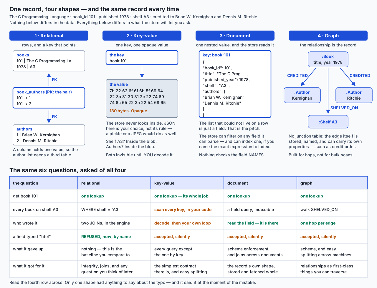
Look at that diagram before reading on, because it is the whole lesson in one picture. The data is identical in all four columns. One book, one year, one shelf, two authors. What differs is entirely what the store will let you ask, and what it will let you get away with.
- Relational stores the book as a row and the two authors as rows in a third table, because a column holds one value and a list will not fit in one. In exchange it will answer any question you think of later, enforce that the author you referenced exists, and refuse the typo at the moment you make it.
- Key-value stores one key,
book:101, pointing at 130 bytes it never looks inside. Fetching by that key is the fastest operation in this lesson. Fetching by anything else — shelf, year, author — is a loop you write, over every key. There is noWHERE. - Document stores the whole book as one nested value, authors list and all, and the store will parse it. So you can filter on a field, and index one. What you cannot do is make it care what the fields are called.
- Graph stores the relationships themselves as first-class objects: a
:Booknode with twoCREDITEDedges. “Who has co-written with Kernighan?” is a traversal rather than a self-join.
And the fourth row of that table is the one to memorise. Given a field typed titel, exactly one of the four had anything to say — and it said it at the moment of the mistake, naming the field.
Historical background
The history is short, well documented, and explains why the word means so little.
Carlo Strozzi used the name “NoSQL” in 1998, for a lightweight open-source database of his own that did not expose a standard SQL interface — but which was still relational. That is worth sitting with for a second: the first thing ever called NoSQL was a relational database. The name referred to the query language, not the model.
The modern meaning arrived a decade later. Johan Oskarsson, then a developer at Last.fm, reintroduced the term in early 2009 when he organised an event to discuss “open-source distributed, non-relational databases”. That phrase is the real definition, and it is much narrower than what the word later came to mean. The systems in the room were largely open-source descendants of two pieces of industrial engineering — Google’s Bigtable and Amazon’s Dynamo — built by companies whose data no longer fitted on one machine and whose access patterns did not need most of what a relational engine was doing for them.
Meanwhile the theoretical result everybody quotes and most people misquote was already in place. Eric Brewer of UC Berkeley formulated it in autumn 1998, published it as a principle in 1999, and presented it as a conjecture at the 2000 Symposium on Principles of Distributed Computing. Seth Gilbert and Nancy Lynch of MIT published the formal proof in 2002, which is what turned a conjecture into a theorem. And in 2012 Brewer himself wrote that the popular “pick two of three” framing is misleading — designers need only sacrifice consistency or availability, and only during a network partition, because partition management and recovery techniques exist. We will come back to that, because getting it right is one of today’s two hardest ideas.
The last chapter of the history is the one that most changes what you should actually do, and it is the least discussed: the relational engines absorbed the good part. The document model’s genuine advantage — store a record whose shape is its own business, query inside it anyway — turned out not to require abandoning the relational model at all. It required a JSON type and some functions.
SQLite is a precise example. Its JSON functions existed for years as an optional extension you had to enable at compile time with -DSQLITE_ENABLE_JSON1. In release 3.38.0, on 22 February 2022, that changed: the release notes state that “the JSON functions are now built-ins” and that “it is no longer necessary to use the -DSQLITE_ENABLE_JSON1 compile-time option to enable JSON support. JSON is on by default.” The same release added the -> and ->> operators, explicitly for compatibility with MySQL and PostgreSQL. PostgreSQL made the same move earlier and further, with a binary JSON type and indexes to match.
So the situation in front of you today is genuinely different from the situation in 2009. Then, “I need to store documents” was a reason to adopt a second database. Now, on a stock SQLite that ships with macOS, it is a column type and four function calls — which you will run for real in about twenty minutes.
What it is — and what it is not
A key-value store is a database whose entire contract is: given a key, store these bytes; given the key again, return them. It does not parse the value, index it, validate it or know anything about it. Redis and Memcached are the well-known ones. Python’s dbm is one too, and it is already installed on your machine.
A document store is a key-value store that agrees to look inside the value. The value must be in a format it can parse — JSON, or a binary encoding of it — and in exchange the store will let you filter and index on fields inside. MongoDB and CouchDB are the well-known ones. You will build one today, in about seventy lines, over sqlite3.
A wide-column store is a store whose unit is a row identified by a partition key, where the columns present may differ per row and rows are grouped physically by that key. Cassandra and HBase are the well-known ones. The design principle is unusual and worth stating plainly: you design the table around the query, not around the data, and if you have two queries you frequently write the data twice.
A graph database stores nodes and edges as first-class objects, so that following a relationship is a pointer hop rather than an index lookup into a join table. Neo4j is the well-known one.
Now the corrections, because almost every one of these is believed by somebody on your team.
| The claim | What is actually true |
|---|---|
| ”NoSQL means no SQL” | Several of these have SQL-like query languages. Cassandra’s CQL is deliberately SQL-shaped. The name is about the model, and only accidentally about the language. |
| ”NoSQL is the opposite of relational” | The first thing ever called NoSQL was relational. And the relational engines now do documents. The two circles overlap heavily. |
| ”Document stores are schemaless” | There is always a schema. The question is only where it lives and who enforces it. In a document store it lives in your application code, is written down in no single place, and is enforced by whoever remembers. |
| ”NoSQL is faster” | Faster at one specific thing: lookup by the key you designed around. Often much slower at anything else, because “anything else” becomes a full scan in your process rather than an index seek in theirs. |
| ”NoSQL scales and SQL does not” | Horizontal scaling is easier when there are no cross-machine joins or foreign keys to enforce. That is a consequence of what was dropped, not a magic property. A single PostgreSQL instance handles far more than most teams who reach for a distributed store will ever have. |
| ”CAP says pick two of three” | It does not, and Brewer said so himself in 2012. See below; this one gets a section. |
| ”Adopting a document store removes the migration problem” | It relocates it. You no longer run ALTER TABLE. You now have documents of six different shapes in one collection and code that must handle all six, forever, because there is no list of which shapes exist. |
The last one is the most expensive misconception in this lesson and the one experienced teams warn about most. Schema changes do not disappear when you stop declaring the schema. They stop being events and become a permanent property of your data.
Why it was created and what problems it solves
Four things genuinely strain the relational model. Not “make it slightly awkward” — genuinely strain it. If your problem is one of these, a different shape may be the right answer. If it is not, it almost certainly is not.
1. A schema that differs per record. You are storing product listings from four hundred suppliers, and each supplier sends a different set of attributes. A shoe has a size; a paint has a volume and a finish; a book has an ISBN. Relationally you have three unappealing options: one enormous table of mostly-NULL columns, a table per product type that you must alter every time a supplier joins, or an entity-attribute-value table which is a document store built badly out of rows. When the variation is genuinely open-ended, a document is the honest representation.
Note the qualifier. Three product types is not open-ended; that is a table with a nullable column or two, and you should write it.
2. Data only ever fetched by one key. A user’s session. A cached rendering of a page. A rate-limit counter. A feature flag. For each of these there is exactly one access pattern, forever: give me the value for this key. You will never say “which sessions started before noon”, because the question is meaningless to the application. Every index, every constraint, every join capability of a relational engine is machinery you are paying for and never using — in memory, in write latency, and in operational complexity.
3. Write volume beyond one machine. When writes exceed what a single machine can absorb, you must split the data across machines. The moment you do, a join across the split becomes a network operation, and a foreign key across the split becomes a distributed transaction. Systems built for this scale drop both — that is what makes them able to split at all. This is a real constraint and a rare one. Be honest about which side of it you are on: it is far more common to be told you have this problem than to have it.
4. Documents whose shape is the point. A CV, a legal contract, a hospital admission form, a survey response. The nesting is not incidental to the record — it is the record. Shredding it into eleven tables to reassemble it with eleven joins on every read is work you do at both ends to gain something you may not need.
Notice the shape of all four arguments. Each one names a specific property of the workload, not a property of the technology. That is how this decision is made. If somebody cannot tell you which of these four they have, they have not made a decision yet.
How it works
The four families, one example each
Key-value. The contract is two operations. Here it is for real, with dbm — a genuine key-value store from Python’s standard library, and everything below was actually executed:
import dbm, json

with dbm.open("library_kv", "c") as store:
    store["book:101"] = json.dumps(book).encode("utf-8")

with dbm.open("library_kv", "r") as store:
    book = json.loads(store[b"book:101"])
Real output from the lab:
backend chosen by Python: dbm.sqlite3
keys: ['book:101', 'book:102', 'book:103', 'book:104']
the value under book:102 is 130 bytes of opaque blob
Redis’s version of the same thing is SET book:101 '{"title":...}' and GET book:101. It adds data structures — lists, sets, sorted sets, hashes — and it holds everything in memory, which is where its speed comes from. No Redis output appears anywhere in this lesson or lab, because Redis is not installed on the machine this was written on and no server was available. The commands are from its documentation; the numbers would be invented, so there are none.
Now the part that matters. Ask that store the same question SQL answers with WHERE published_year < 1990:
--- 2. get by key: one lookup, no scan ---
keys examined: 1

--- 3. the same question as SQL's WHERE published_year < 1990 ---
    there is no WHERE. You write the loop.
    101  The C Programming Language
    102  The Mythical Man-Month
keys examined: 4 of 4 (every key in the store)
json.loads calls: 4 (every value decoded, matching or not)
One versus all. With four books that is a joke; with four million it is your afternoon. And the fix — a secondary index — is a fix you build and maintain yourself:
--- 4. the usual fix: a secondary index you maintain yourself ---
index:decade:1970s -> [101, 102]
keys examined: 3 (one index key, then one key per hit)
Then the bill for that fix, demonstrated rather than warned about:
--- 5. delete a book and forget the index ---
index:decade:1970s still lists [101, 102]
ids in that index with no book left in the store: [102]
no error was raised at any point
That is an orphaned reference — the exact thing a foreign key exists to prevent — recreated by hand, in eight lines, with the database entirely at peace about it.
Document. The contract adds one operation: find by a field inside the value. MongoDB’s is db.books.find({ shelf: "A3" }). Ours, built today, is store.find("shelf", "A3"). Same idea. Again: no MongoDB output appears here, for the same reason.
Wide-column. Cassandra’s data model is a partition key that decides which machine holds the row and where it sits on disk, plus clustering columns that decide the order within the partition. A table declaration looks SQL-ish:
CREATE TABLE loans_by_member (
  member_id   uuid,
  borrowed_at timestamp,
  book_id     uuid,
  title       text,
  PRIMARY KEY (member_id, borrowed_at)
);
The thing to notice is title. It is copied into this table from wherever books live, because there is no join to fetch it with. And if you also need loans by book, you create a second table, loans_by_book, and write every loan twice. That is not a hack; it is the documented design method. You model the query. Nothing here was run against Cassandra; no server was available.
Graph. Neo4j’s query language, Cypher, describes a shape and asks for everything matching it:
MATCH (a:Author)-[:CREDITED]->(b:Book)<-[:CREDITED]-(other:Author)
WHERE a.name = 'Brian W. Kernighan'
RETURN other.name
Relationally that is a self-join through the junction table, which is writable but gets ugly fast at three or four hops. In a graph store each hop is a pointer. Not run here either.
Schema-on-write against schema-on-read — and who pays when
This is the trade at the centre of the day, and the useful way to state it is not “strict versus flexible”. It is who pays, and when.
| Schema-on-write | Schema-on-read | |
|---|---|---|
| Where the shape is declared | In the database, once, in one place | In application code, in as many places as read it |
| Who enforces it | The engine, on every write, without exception | Whoever remembered to write a check |
| When you find out about a mistake | At the moment of the mistake, with the field named | Later. Possibly much later. Possibly via a wrong number |
| What a mistake costs | One rejected statement | An unknown number of bad records and an archaeology project |
| Cost of adding a field | A migration: planned, reviewed, deployed | Nothing. Write the new shape and move on |
| Cost of having added a field | Nothing. Every row has it | Every reader must now handle both shapes, forever |
| Where the pain concentrates | At change time, visibly, on a Tuesday | At read time, invisibly, spread over years |
Both columns are real. The second column’s top half is why document stores are pleasant to start with, and its bottom half is why teams five years in write validation layers that reimplement the first column badly.
The honest summary is one sentence: the schema never went away — it moved from a place that enforces it to a place that hopes.
The joins you now do yourself, and the denormalization that follows
Drop cross-document joins and one of two things happens.
Either you do the join in application code, which means a second round trip:
loan = store.get("loan:1")
book = store.get(f"book:{loan['book_id']}")   # a second query, over the network
Do that inside a loop over a hundred loans and you have made a hundred and one queries. It is the classic N+1 problem, and here you cannot fix it with a join, because there is no join.
Or you avoid the round trip by copying the title into the loan document. That is denormalization, and it works — reads become one lookup. The bill arrives when a title changes. Now one fact lives in one book document and in every loan document that ever referenced it, and updating it means finding them all. There is no UPDATE ... WHERE, no cascade, no constraint, and no error if you miss one. You just have two spellings of the same book in your database and no way to know which is current.
This is the update anomaly that normalization was invented to prevent, in 1971, re-entering through a different door.
CAP, stated correctly
Almost every explanation you will read of the CAP theorem is wrong in the same way, so it is worth being precise. First, the three terms as they are formally defined:
- Consistency — every read receives the most recent write, or an error.
- Availability — every request received by a non-failing node results in a response (with no guarantee that it reflects the most recent write).
- Partition tolerance — the system continues to operate despite an arbitrary number of messages being dropped or delayed by the network.
Now the theorem, stated as the result actually is: when a network partition occurs, a distributed data store cannot provide both consistency and availability. It must give up one of them, for as long as the partition lasts.
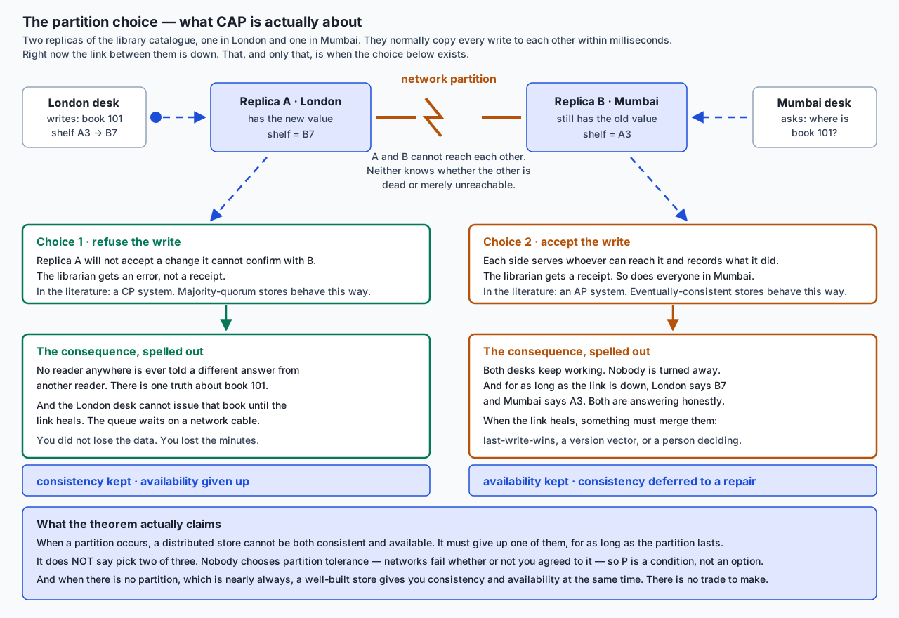
What is wrong with “pick two of three”:
You do not pick P. The network picks. Cables are cut, switches reboot, a data centre loses a link. Partition tolerance is not a feature you select; it is a condition you are subjected to. A distributed system that “chose CA” is a system that has chosen to be broken when the network is.
There is no trade when there is no partition. This is the part that surprises people, and it is Brewer’s own 2012 clarification: a well-built store gives you consistency and availability at the same time, essentially always, because essentially always there is no partition. The choice exists only during the failure, and the failure is a small fraction of any year.
The choice is operational, not philosophical. Follow the diagram. A librarian in London moves a book from shelf A3 to B7. The link to the Mumbai replica is down. There are exactly two things the system can do:
- Refuse the write. Nobody is ever told two different answers. The price is that the London desk cannot issue that book until the cable is repaired — the queue waits on a network fault. This is what a majority-quorum system does.
- Accept the write. Both desks keep working. The price is that for the duration, London says B7 and Mumbai says A3, both honestly, and when the link heals something must merge them: last-write-wins, a version vector, or a person deciding.
Neither is the right answer in general. For a shopping cart, take the write — a customer who cannot add an item leaves. For the seat allocation on a flight, or the balance of a bank account, refuse it. The question is not “which does my database do?” but “what does my business want to happen at 3am when the cable is cut?”, and that is a product decision that got mislabelled as a technical one.
And the practical footnote: none of this applies to a single-machine database. SQLite has no partitions because it has no network between replicas. If your data lives on one machine, CAP is trivia. It becomes real the moment you have two.
From scratch: a document store in seventy lines
The fastest way to stop treating “NoSQL” as a category of magic is to build one. Here is the whole thing, over sqlite3:
class DocumentStore:
    def __init__(self, path):
        self.connection = sqlite3.connect(path)
        self.connection.execute(
            "CREATE TABLE IF NOT EXISTS documents ("
            "  key  TEXT PRIMARY KEY,"
            "  body TEXT NOT NULL CHECK (json_valid(body)))"
        )
        self.connection.commit()

    def put(self, key, document):
        self.connection.execute(
            "INSERT INTO documents (key, body) VALUES (?, ?) "
            "ON CONFLICT(key) DO UPDATE SET body = excluded.body",
            (key, json.dumps(document)),
        )
        self.connection.commit()

    def get(self, key):
        row = self.connection.execute(
            "SELECT body FROM documents WHERE key = ?", (key,)
        ).fetchone()
        return None if row is None else json.loads(row[0])

    def delete(self, key):
        cursor = self.connection.execute("DELETE FROM documents WHERE key = ?", (key,))
        self.connection.commit()
        return cursor.rowcount > 0
That is a key-value store. Two more methods make it a document store — the difference being that it now looks inside the value:
    def _path(self, field):
        if not SAFE_FIELD.match(field):          # ^[A-Za-z_][A-Za-z0-9_]*$
            raise ValueError(f"not a safe field name: {field!r}")
        return f"json_extract(body, '$.{field}')"

    def find(self, field, value):
        sql = f"SELECT body FROM documents WHERE {self._path(field)} = ? ORDER BY key"
        return [json.loads(row[0]) for row in self.connection.execute(sql, (value,))]

    def create_index(self, field):
        self.connection.execute(
            f"CREATE INDEX IF NOT EXISTS idx_docs_{field} "
            f"ON documents ({self._path(field)})"
        )
        self.connection.commit()
Two things in that code are not decoration.
The SAFE_FIELD check exists because the field name is interpolated into SQL text rather than bound as a parameter, and it has to be: a JSON path passed as a bound parameter defeats the expression index, because the planner can no longer see that the query’s expression matches the index’s expression. Anything interpolated into SQL must come from an allow-list you wrote. The lab’s test suite calls find("shelf'); DROP TABLE documents; --", "A3") and asserts a ValueError.
The CHECK (json_valid(body)) is the entire remaining schema. It says the blob parses. It says nothing whatever about which fields it has.
Now the measurement, from a real run with 20,004 documents loaded:
plan without the index: SCAN documents
plan with the index:    SEARCH documents USING INDEX idx_docs_shelf (<expr>=?)
find('shelf', 'F137') returned 50 documents both times: True
without index:    5.779 ms per call
with index:       0.066 ms per call
ratio: 88x
A repeat run on the same machine gave 95x, so treat the number as an order of magnitude rather than a constant — your machine will differ and that is expected. What does not vary is the plan changing from SCAN to SEARCH, and that the answer is identical both times. An index changes speed, never results.
Then the second half of the exercise, which is the more valuable half — what you did not get:
(a) no schema enforcement: the misspelled document is accepted
    get('book:105') -> ['authors', 'book_id', 'published_year', 'shelf', 'titel']
    find('shelf', 'C1') finds it: 1 document
    find('title', 'Compilers: Principles, Techniques, and Tools') -> []
    the book is in the store and the title query cannot see it

(b) no referential integrity: a loan may point at a book that is gone
    put a loan for book_id 999, which does not exist -> accepted

(c) no join: relating two documents is a second round trip in Python

(d) no cross-document transaction unless you write one
Point (d) has a twist worth noticing. This store can do an atomic multi-document write — the lab demonstrates a rollback — but only because it is built on a relational engine that already had transactions. That capability was inherited, not designed in. A distributed document store spread over twenty machines does not get it for free, which is precisely why cross-document transactions were among the last features such systems gained.
JSON inside a relational database — the middle path
Now the option most teams should try first, and the one that barely existed when this whole debate started.
CREATE TABLE documents (
  doc_id INTEGER PRIMARY KEY,
  body   TEXT NOT NULL CHECK (json_valid(body))
);
Real output, from the stock sqlite3 on the authoring machine:
--- 1. reach inside the document with json_extract ---
doc_id  title                                       year
------  ------------------------------------------  ----
101     The C Programming Language                  1978
102     The Mythical Man-Month                      1975
103     Artificial Intelligence: A Modern Approach  1995
104     The Practice of Programming                 1999
The -> and ->> operators say the same thing more briefly, and they differ in a way worth knowing:
doc_id  arrow_json  arrow_type  arrow2_value  arrow2_type
------  ----------  ----------  ------------  -----------
101     1978        text        1978          integer
-> returns JSON — so a JSON number comes back as JSON text, and a JSON string comes back still quoted. ->> returns a SQL value with a SQL type. Use ->> when you want to compare, sort or sum; use -> when you want to keep drilling.
json_each unrolls the nested array that needed a whole junction table an hour ago:
SELECT author.value AS author, count(*) AS books
  FROM documents, json_each(documents.body, '$.authors') AS author
 GROUP BY author.value ORDER BY books DESC, author;
author books
----------------------- -----
Brian W. Kernighan 2
Dennis M. Ritchie 1
Frederick P. Brooks Jr. 1And the index, which is what makes this a serious option rather than a party trick:
--- 5. what the planner does without an index ---
`--SCAN documents

--- 6. an index on an EXTRACTED field, then the same plan again ---
`--SEARCH documents USING COVERING INDEX idx_documents_shelf (<expr>=?)
One catch, and it caught me while writing this, so it is in the lab as a numbered step:
--- 7. the catch: the index only helps the EXACT expression it indexes ---
`--SCAN documents
That is the same question — WHERE body ->> '$.shelf' = 'A3' instead of WHERE json_extract(body, '$.shelf') = 'A3' — and the index does not apply, because an expression index matches an expression, not an intention. Pick one spelling and use it in the index and in every query.
What you keep by taking this path: transactions, foreign keys on the columns you did declare, joins to your ordinary tables, one database to back up, and every SQL skill from Week 13. What you give up: the store still does not check the field names inside body. That is unavoidable, and the reason schema-on-read is a property of the document model rather than of any particular product.
An everyday analogy
Picture one archive room, and four ways of filing the same case papers. Keep this room in your head for the rest of the lesson; every trade-off in it maps onto something above.
The card catalogue with cross-references — relational. Every fact is written on exactly one card. The case card names the client by number; the client card holds the name. To learn who the client on case 4471 is, you follow the number to the other drawer. Filing a new case takes longer, because the form insists on every field and refuses a client number nobody has issued. In exchange, when the auditor asks a question nobody anticipated — “every case opened in March for clients in Leeds” — you can walk to the drawers and answer it. The cost is up front, in discipline. The benefit is that any question is answerable.
The wall of numbered lockers — key-value. Each locker holds one sealed envelope. If you know the number, you have the papers in two seconds; it is the fastest thing in the room and nothing about it can go wrong. If you do not know the number, you have to open every locker. There is no drawer of numbers unless you keep one — and if you do, you keep it. Nobody updates it when a locker is emptied. That is exactly the stale index from the lab.
The shelf of case folders — document. One folder per case, holding everything: the client’s name, the correspondence, the dated notes, all in one place. Pull the folder and you have the case; no cross-referencing, no second drawer. The clerk can also flick through the folders looking at, say, the county on the front sheet, and if that question is common enough she keeps a tab index by county on the shelf edge. Two costs, both real. The client’s name is now written inside forty folders, so when she marries you have forty folders to correct, and no list of which forty. And nothing stops a junior writing “Country” where the form says “County”: the folder is filed, the tab index does not pick it up, and the folder is invisible to that search forever.
The pinboard of strings — graph. Cards on a board with coloured string between them: this solicitor worked with that client on this case. To answer “who has worked with whom, two removes out?”, you follow strings with your finger, which takes seconds. Doing the same from the card catalogue means walking between drawers repeatedly. But ask “how many cases opened in March?” and the pinboard is the worst tool in the room, because you must inspect every card.
Where the analogy holds well: the placement of effort. The catalogue front-loads it into filing; the lockers eliminate it for one question and dump it on you for every other; the folders trade duplication for retrieval; the pinboard trades bulk queries for traversal.
Where it stops, and this matters: a room has no partitions. Two rooms does. Build a second archive in another city, keep them in step by courier, and now ask what happens on the day the courier cannot get through — refuse to file anything until he does, or file on both sides and reconcile later? That is the CAP diagram exactly, and notice that the answer depends entirely on what the papers are for.
Examples in practice
Key-value stores are not a compromise. For a specific and common set of jobs they are exactly right, and each has a standard pattern. These are the five worth knowing, with what makes them fit.
1. Caching. Key: something that identifies the derived thing — page:home:v3, user:88:profile. Value: the rendered output. Two properties make this a perfect fit: you always know the key, and being wrong is survivable, because a cache miss recomputes. Every cache entry gets an expiry; the store evicts on its own schedule. Redis’s SET key value EX 300 sets a value that expires in 300 seconds, and its documentation describes several eviction policies for when memory fills, including least-recently-used. The hard problem in caching has never been the store — it is invalidation, and the store cannot help you with it.
2. Sessions. Key: the session id from the cookie. Value: whatever the session holds. Nothing else ever queries it — “list all sessions for user 88” is a question you should not be answering this way — and expiry is the logout. Putting sessions in a relational table works and is common; putting them in a key-value store means your main database does not absorb a write on every page view.
3. Rate limiting. Key: rate:{user}:{minute}. Increment on each request, reject above the threshold, let the key expire when the minute passes. What makes this work is that the increment is atomic in the store, so two concurrent requests cannot both read 9 and both write 10. Doing it correctly in an application, over a store without an atomic increment, is a race condition waiting to happen.
4. Feature flags. Key: flag:new-checkout. Value: on, off, or a percentage. Read constantly, written rarely, and needing to be fast because it is on the path of every request. The pattern is a local in-process cache in front of the store with a short refresh, so that the store’s availability does not become your application’s availability.
5. Queues and work lists. A list structure with push and pop, where the pop is atomic so two workers never take the same job. Redis’s list commands are used this way constantly. The caveat is honest and important: a simple POP removes the job before it is done, so a worker that crashes loses it. Real queues need acknowledgement and a way to redeliver, and if you need that, use a queue rather than building one — which is a fair summary of most “we built it on Redis” stories.
The unifying pattern in all five: there is exactly one access pattern and you always know the key. When you can say that sentence honestly about your data, a key-value store is not a compromise, it is the correct tool. When you cannot, you are about to write a lot of loops.
And the thing you can run today, which is the reason dbm is in this lab rather than a paragraph about Redis: every one of those patterns is bytes addressed by a key, and you can feel the whole trade-off — the one-key lookup, the all-keys scan, the index you maintain, the index going stale — on a machine with nothing installed.
Implications: security, privacy, performance, scalability, and cost
Security and privacy. The consequence people miss is that the document model moves your sensitive fields. In a relational schema, members.email is a place: one column, one table. Ask “where do we hold email addresses?” and the schema answers. You can grant on it, revoke on it, encrypt it, redact it or drop it. In a document store the same address is a key inside a blob in a column called body, and three things follow. You cannot grant access to part of a document, so column-level privileges have nothing to bite on. You cannot enumerate what you hold, because there is no list of fields — finding every place a phone number is stored means scanning every document and inferring. And a new field can appear with no ceremony at all, so the first anybody knows that you now store dates of birth is when someone greps for it.
That is a data-protection problem, not a database problem, and it is the same sentence as schema-on-read aimed at a different audience: the check moved from the engine to somebody’s job.
Two more, briefly. Never store a pickle you did not create — a key-value store’s value is opaque, which makes it exactly the kind of place where bytes arrive from elsewhere, and unpickling untrusted bytes executes code. Use JSON. And deletion has no cascade: “delete my account” removes the user key and leaves their address in every secondary index and every denormalized copy, none of which the store knows about.
Performance. Two real numbers from today, both measured. The key-value store examined 1 key for a lookup by key and 4 of 4 for a lookup by anything else. The document store’s find took 5.779 ms unindexed and 0.066 ms indexed on 20,004 documents, an 88x difference on one machine on one day, with a repeat run giving 95x. The stable fact is the plan: SCAN became SEARCH.
The general shape is this. Key-value is fast because it does less — no parsing, no index maintenance on write, no constraint checking. Document stores give some of that back the moment you add indexes, because every index is work on every write. And a full scan is a full scan in any store; the difference is whether it happens in a tuned C engine next to the disk, or in your Python process after a network round trip per document.
Scalability. Two mechanisms are worth naming precisely, because they are often confused. Sharding splits data across machines by a key, so each machine holds a slice; it increases capacity and it is what makes a cross-shard join a distributed problem. Replication copies the same data to several machines; it increases read capacity and survives a machine failure, and it is what makes the CAP choice exist at all. You can have either, both or neither, and they solve different problems: sharding for volume, replication for availability.
The honest scaling note: a single well-indexed relational database on modern hardware handles more than most teams will ever need. The number of organisations that genuinely cannot fit on one machine is much smaller than the number that have adopted a distributed store.
Cost. No prices appear in this lesson, because prices change and a fabricated one is worse than none. What is stated safely is the shape of the cost, and the shape is that the licence is usually the smallest part. A second datastore is a second thing to back up, restore-test, monitor, secure, patch, upgrade and be paged about; it is a second set of client libraries in your dependency tree, a second failure mode in every incident, and a second body of knowledge your team must keep. Memory-resident stores like Redis add a specific cost, which is that memory is expensive and your dataset must fit in it, or you must configure what gets evicted when it does not.
Against that: the option you already have costs nothing to try. SQLite’s JSON support is in the binary on your machine. That asymmetry is the practical argument for the middle path, and it is stronger than any benchmark.
Alternatives: free, open source, and commercial
Below is each notable option with when to choose it, how you use it, one concrete example, and its free-versus-paid shape. First, the honesty statement, because it governs the whole section: of everything named here, I ran only SQLite, Python’s dbm, and the document store built in the lab. Redis, Memcached, MongoDB, CouchDB, Cassandra, HBase, Neo4j and DynamoDB were not installed and no server was available. Their commands are taken from their published documentation. No output is reproduced for any of them, because it would have to be invented.
SQLite with JSON — the one to try first.
When: you need per-record flexibility for part of your data, your data fits on one machine, and you would like to keep transactions and joins.
How: a TEXT column with CHECK (json_valid(body)), then json_extract, ->>, json_each, and an index on the extracted expression.
Example: everything in the “middle path” section above — run, captured, in the lab.
Cost: free, public domain, already installed. No server, no operations.
PostgreSQL with JSON — the same idea at production scale.
When: you outgrow SQLite’s single-writer model, or want concurrent writers, real date and boolean types, and richer JSON indexing.
How: the same shape, with a binary JSON type and index types built for containment queries.
Example: a products table with declared columns for what every product has and a JSON column for the supplier-specific attributes — the hybrid design most teams should reach for before adopting a document database.
Cost: free and open source; commercial managed hosting from many vendors if you would rather not run it.
Redis — the key-value store to reach for.
When: caching, sessions, rate limits, flags, ephemeral queues; anything where you always know the key and want it fast.
How: SET/GET plus data structures — hashes, lists, sets, sorted sets — and expiries per key.
Example: SET rate:user88:1421 1 EX 60 then increment per request and reject over the threshold. The atomic increment is the whole reason it works.
Cost: free editions exist and there are open-source forks; managed services from cloud vendors are paid. Its licensing has changed more than once recently and differs between server, modules and managed offerings, so check the current terms rather than trusting any summary — including this one.
Memcached — the smaller, older cache.
When: you want a cache and only a cache, distributed across several machines, with the simplest possible operational story.
How: set, get, delete, with expiry. No data structures, no persistence.
Example: caching rendered fragments across a fleet of web servers.
Cost: free and open source. Choose it over Redis when you want less, not more; choose Redis when you want the data structures or persistence.
MongoDB — the document store people mean when they say “NoSQL”.
When: genuinely open-ended per-record shape, and a team that will maintain validation in application code.
How: collections of documents; find with a field predicate; indexes on fields including nested paths; aggregation pipelines for grouping.
Example: db.books.find({ shelf: "A3" }), which is store.find("shelf", "A3") in the store you build today.
Cost: a free community edition to self-host and a paid managed cloud service. Licensing differs between the server and the drivers; check current terms.
CouchDB — the document store built around replication. When: occasionally connected clients that must work offline and merge later — field data collection, mobile-first apps. How: an HTTP API, documents with revisions, and a replication protocol designed for conflict handling as a normal event rather than an error. Example: survey apps that collect on a tablet with no signal and sync when there is one. Cost: free and open source.
Cassandra — the wide-column store for write volume.
When: write rates beyond one machine, across data centres, where you can enumerate your queries in advance.
How: CQL; a partition key that chooses the machine; clustering columns for order within the partition; a table per query pattern.
Example: the loans_by_member table above, plus a loans_by_book table holding the same data again.
Cost: free and open source, with commercial distributions and managed services available.
HBase — the wide-column store on the Hadoop stack. When: you are already running Hadoop and want random read and write over data that also feeds batch jobs. How: row key design decides everything; scans over key ranges. Example: time-series rows keyed by entity plus a reversed timestamp so the newest sorts first. Cost: free and open source. Choose it for Hadoop integration, not on its own merits.
Neo4j — the graph database. When: the relationships are the product. Recommendations, fraud rings, dependency and impact analysis, knowledge graphs. How: Cypher, which draws the pattern you want in ASCII arrows and returns everything matching. Example: the co-authorship query above — trivial to write, and increasingly painful as a relational self-join at three or four hops. Cost: a free community edition and paid enterprise and cloud editions.
DynamoDB — the managed key-value and document store. When: you are on AWS, want no servers to run, and can design around a partition key. How: tables with a partition key and optional sort key; secondary indexes declared explicitly; capacity provisioned or on demand. Example: a sessions table keyed on session id with a time-to-live attribute, so expiry is the database’s job. Cost: commercial and usage-metered, with a free tier that has changed over time — check the current terms rather than any figure quoted anywhere, including here.
And the free option you already have, which is the point of the lab: Python’s dbm. A real key-value store, in the standard library, which forces exactly the same trade Redis forces, and which you can measure today.
Comparison with related concepts
| Concept | What it actually is | How it differs from today’s topic |
|---|---|---|
| Relational database | Tables, declared columns, keys, joins, transactions | Not the opposite of NoSQL: it now does documents too, which is why the middle path exists |
| Key-value store | Opaque value addressed by one key | The simplest contract there is; a document store is this plus “and I will parse the value” |
| Document store | Key-value where the value is parseable and queryable | Adds field queries and indexes; still does not check field names |
| Wide-column store | Rows grouped by partition key, columns varying per row | Not a document store; the unit is a row on a specific machine, and you model the query rather than the data |
| Graph database | Nodes and edges as first-class stored objects | Optimised for traversal, not for bulk scans; the opposite trade from wide-column |
| NewSQL | Distributed engines offering SQL and transactions across machines | The attempt to get the scaling without giving up the relational guarantees |
| Data warehouse | Column-oriented store for analytics over history | Also “not a normal relational database”, for a completely different reason: analytical scans, not per-record flexibility |
| Object storage | Files addressed by a name, with no query capability at all | A key-value store for large blobs; often where a document store’s attachments actually live |
| Cache | A store you are allowed to lose | Usually key-value, but the defining property is expendability, not shape |
| Vector database | Nearest-neighbour lookup over embeddings | A key-value store whose key is a vector and whose lookup is “closest”, not “equal” |
| Feature store | Values keyed by entity and time | A key-value store with time semantics bolted on: “what did we know about user 88 as of last Tuesday?” |
The last two are today’s AI thread in table form, and they are worth reading twice, because they demystify two things that are usually presented as new categories.
When to use it — and when not to
Reach for a key-value store when there is exactly one access pattern and you always know the key; when the data is expendable or rebuildable; when you need an atomic counter or an expiry; when it is a cache, a session, a rate limit, a flag or a work list.
Reach for a document store when the record’s shape genuinely varies per record and the variation is open-ended rather than three known cases; when the document is the natural unit of both read and write; when you will actually build and maintain the validation layer that the store does not provide.
Reach for a wide-column store when write volume genuinely exceeds one machine and you can enumerate your query patterns in advance, accepting that you will write the data once per pattern.
Reach for a graph database when the questions are about paths and connections rather than about aggregates, and the joins in your relational version have already reached three or four hops.
Reach for JSON in your relational database when — and this is most of the time — one part of your data needs flexibility, the rest does not, everything fits on one machine, and you would like to keep transactions, foreign keys, joins and one system to operate.
Do not reach for any of them when:
- The reason is that relational feels old-fashioned. That is not a requirement.
- You have not measured. “It will be faster” is a hypothesis, and the machine in front of you can test it in an afternoon.
- The variation is three known cases. That is a nullable column or a type table, and you already know how to write both.
- You need a report you have not thought of yet. Ad-hoc questions are what the relational model is for, and giving that up to gain a lookup you could already do quickly is a bad trade made confidently.
- Somebody said “web scale”. Ask which of the four strains they have. If they cannot name one, the decision has not been made yet.
- You would be adopting a second datastore to hold part of one dataset that must stay consistent with the rest. There is no transaction spanning the two, and you have just invented a class of bug with no automatic detection.
The default that will serve you well for years: start relational; use its JSON support when part of the data varies; add a key-value store when a specific access pattern earns it; and only distribute when a measurement, not an aspiration, says you must.
Now the AI thread, and it is more literal than usual today.
A vector database is a specialised key-value store. The key is an embedding, and the lookup is nearest-neighbour rather than exact match. Everything you learned about key-value stores today transfers directly: it is superb at the one question it was built for, and any other question — “which chunks came from documents published after 2024?” — is a filter you must either bolt on or answer by scanning. That is why every serious vector store has grown metadata filtering, and why filtering interacts awkwardly with the index: it is the secondary-index problem from this morning’s lab, in a harder setting.
A feature store is a key-value store with time semantics. The key is an entity, the value is its features, and the extra requirement is “as of when” — because a model trained on values that were not yet known at prediction time will look excellent in evaluation and fail in production. That is the same store you built today, with a version dimension.
And the metadata beside every chunk in a retrieval system is a document. Source, page number, ingestion timestamp, licence, chunker version. Nobody enforces its shape, because the store you chose does not enforce shapes. So when a scraper starts writing pageno instead of page_number, every filter on page number silently stops matching those chunks, no error appears anywhere, and retrieval quality drops for a reason no metric will name. That is exactly the titel document from this lesson, in the system you are going to build later in this course — which is why the day spends its energy on making you watch a store accept a mistake in silence, rather than on a tour of product names.
Knowledge check
Try these from memory before looking back.
- Complete the sentence: “NoSQL is not one thing, and it is not ___.” Then say what the four families actually have in common.
- What are the two questions that replace “SQL or NoSQL?”, and in what order?
- Name the four families and, for each, the guarantee it gives up and the thing it gets in exchange.
- A key-value store answers a lookup by key in one operation. How many does it take to answer “every book on shelf A3”, and where does that work happen?
- You build a secondary index by hand over a key-value store. Describe the failure the lab demonstrates, and say what relational feature exists to prevent exactly that.
- State schema-on-write and schema-on-read in terms of who pays and when. Where does the schema go when you stop declaring it?
- Give the two ways to handle a join you no longer have, and the specific cost of each.
- State the CAP theorem correctly, in one sentence. Then give the three things wrong with “pick two of three”.
- During a partition, what are the two options and what is the concrete consequence of each? Give a workload for which each is the right answer.
- Why is CAP irrelevant to SQLite?
- What do
->and->>return differently in SQLite, and which do you use for a comparison? - You create an index on
json_extract(body, '$.shelf')and your query still saysSCAN. Give two possible reasons. - Name the four things the from-scratch document store does not give you. Which one does it partly have anyway, and why does that not generalise?
- Give five jobs a key-value store is exactly right for, and the pattern for each.
- In what sense is a vector database a key-value store? What problem does that immediately predict it will have?
Hands-on exercise
The Day 92 lab, One Domain, Four Shapes, models the same library four ways and measures the consequences. Work in the lab directory; everything runs offline and nothing needs installing.
First confirm your SQLite has what the lab needs — this is a real check, not a formality, because JSON support was optional before 3.38.0:
cd labs/sections/programming-with-python/day-092-beyond-tables-nosql-and-key-value
sqlite3 :memory: "SELECT sqlite_version(), json_extract('{\"a\":1}','\$.a'), '{\"a\":2}' ->> '\$.a', (SELECT count(*) FROM json_each('[1,2,3]'));"
Then work through the four shapes in order, giving the examples a scratch directory:
work=$(mktemp -d)
sqlite3 "$work/library.db" < examples/01_relational.sql
python3 examples/02_key_value_dbm.py "$work"
sqlite3 "$work/docs.db" < examples/03_json_in_sqlite.sql
python3 examples/04_docstore.py "$work"
python3 examples/05_schema_on_read.py "$work"
Then build the store yourself. starter/01_exercises.py has five exercises, each a single line, each shipped as a working line that is wrong in one named way — so the file always runs and always tells you what is still wrong:
python3 starter/01_exercises.pyExercise 1 is get. Exercise 2 is find, using json_extract. Exercise 3 is the index on the extracted expression — and note that creating an index is not enough, it must be on the same expression the query uses. Exercise 4 is missing_fields, which is the schema check the store does not perform for you. Exercise 5 is the audit query that finds documents with no title, which is the whole of what you have instead of a schema.
Finish with the harness:
bash tests/run_tests.sh
echo "exit code: $?"
rm -rf "$work"
Expected output
The first example exits 1 on purpose, and that is the control case for the whole lab:
--- 4. schema-on-write: a misspelled column is refused, now, loudly ---
Parse error near line 116: table books has no column named titel
The key-value store reports the trade as two numbers — keys examined: 1 for the lookup by key, keys examined: 4 of 4 (every key in the store) for the lookup by anything else — and then shows its hand-built index going stale with ids in that index with no book left in the store: [102] and no error was raised at any point.
The JSON example shows arrow_type as text against arrow2_type as integer, then three query plans: SCAN documents, then SEARCH documents USING COVERING INDEX idx_documents_shelf, then SCAN documents again for the same question spelled with ->>.
The from-scratch store reports the plan changing from SCAN documents to SEARCH documents USING INDEX idx_docs_shelf, find('shelf', 'F137') returned 50 documents both times: True, and a speedup around 88x on the authoring machine — your timings will differ, and a repeat run here gave 95x. The plan change does not differ.
And the punchline:
store                             the write   stored  query finds it
--------------------------------  ----------  ------  --------------
relational (books table)          REFUSED     4       no
key-value (dbm)                   ACCEPTED    5       no
JSON documents in SQLite          ACCEPTED    5       no
the from-scratch document store   ACCEPTED    5       no
The starter reports 0 of 5 exercises complete. with exit 1 before you begin and 5 of 5 exercises complete. with exit 0 when you are done. The harness ends with the real captured line:
67 checks, 0 failure(s).and exits 0.
Validate your work
bash tests/run_tests.shprints67 checks, 0 failure(s).andecho $?shows0.python3 starter/01_exercises.pyprints5 of 5 exercises complete.and exits 0.- The relational example still refuses the typo and the table still holds exactly 4 books afterwards.
- In the from-scratch store,
findreturns the same documents before and after the index. If the count changed, the index is not the thing that changed the answer and something else is wrong. find('shelf', 'C1')finds the malformed document whilefind('title', ...)does not. Both halves matter: the document is stored and invisible. A store that had rejected the write would also return zero rows, so testing only the second half would prove nothing.- Exercise 5’s audit returns exactly
['book:105']. - Nothing is left behind: no
.dbfile and no__pycache__in the lab directory. The final section of the harness asserts this.
Troubleshooting
no such function: json_extract— your SQLite predates 3.38.0, when the JSON functions became part of the default build. Check withsqlite3 --version. Note that the shell and the copy inside Python are two separate installations and can differ; on the authoring machine they were 3.51.0 and 3.53.3.examples/01_relational.sqlexits 1 — correct, and the point of the file. If it ever exits 0, the comparison has lost its control case.- A query returns zero rows and you are certain the document is there. It probably is. Look for the field, not the value:
WHERE json_extract(body, '$.title') IS NULL.json_extractreturns SQLNULLfor a field that does not exist, andNULL = 'anything'is never true, so a misspelled field produces silence rather than an error. - The plan still says
SCANafter you created the index. Either the indexed expression is not the queried expression —json_extract(body, '$.shelf')andbody ->> '$.shelf'are different expressions asking the same question — or the table is too small for an index to beat a scan, which is why the lab loads 20,000 documents before timing anything. ValueError: not a safe field name— the allow-list did its job. Field names are interpolated into SQL, so they must be plain identifiers.dbm.whichdbreports something other thandbm.sqlite3— expected. Python picks a backend when it creates the file, and it differs by platform and version. Nothing in the lab depends on which one you get.
troubleshooting.md in the lab covers every error message this lab can produce, grouped by where you hit it.
Common mistakes
- Testing only that the malformed document is invisible. Zero rows is also what a store that rejected the write returns. Assert both: it is stored, and it cannot be found.
- Asserting a millisecond figure. Timings move with the machine, the disk and whatever else is running. Assert the plan (
SCANtoSEARCH) and a generous floor on the ratio. - Creating an index on the wrong expression and concluding that expression indexes do not work. They work exactly, and only, for the expression you indexed.
- Comparing to
NULLwith=.json_extract(...) = NULLis never true. UseIS NULL. - Interpolating a field name that came from user input. The value is a bound parameter; the field name has to be interpolated, which is precisely why it must be checked against an allow-list first.
- Concluding that document stores are bad. The lab is not an argument against them. It is an argument for knowing which guarantee you dropped. Three of the four shapes accepting the typo is the price of the flexibility they offer, and for some workloads that is a price worth paying — knowingly.
- Leaving a
.dbfile in the lab directory because you ran an example without a scratch directory. Give them$(mktemp -d).
Practice assignment
Take one system you have actually used — a to-do app, a shop, a course platform, a chat tool — and produce a two-page storage design for it. This is the exercise that turns today from vocabulary into judgement.
- List the data. Every kind of record the system holds. Users, items, sessions, events, settings, uploads.
- For each one, write its access patterns. Not “we query it” — the actual questions, in the words the product uses. “Fetch the cart for this session.” “List every order this month over £50.” “Show the five most recent messages in this room.”
- For each one, name the shape you would choose and the guarantee you are giving up. Use the four-column table from the diagram. If you choose relational, say so — that is a decision too, and it will be the right one for most rows.
- Find at least one item where a key-value store is genuinely correct, and state which of the five patterns it is: cache, session, rate limit, flag, or queue. If you cannot find one, say so and explain why; that is a legitimate finding.
- Find at least one item where a document is the honest shape, and prove it by writing out two records that would have different fields. If both records have the same fields, you have found a table.
- Write the validation you would need for that document, as a list of required fields — and then write, in one sentence each, where in the code it would run and what happens to the documents written before you added it.
- Answer the partition question. If this system ran in two regions and the link between them failed for ten minutes, which writes would you refuse and which would you accept? Give a reason per record type. The answer will not be the same for all of them, and noticing that is the point.
Then, the reality check: implement the smallest one of these in the lab’s DocumentStore. Twenty minutes. A design you have not typed is a design you have not tested.
Extension challenge
Pick one. Each is a genuine piece of engineering and each has a payoff you can measure.
1. Make the stale index impossible — and then find the hole. Rewrite the lab’s dbm example so deleting a book also repairs the decade index. Then ask the question the fix does not answer: what if the process dies between the two writes? Write down what a key-value store offers to prevent that, what it does not, and what a relational engine would have done instead in one word.
2. Add nested paths to the document store. Right now find handles top-level fields only, because SAFE_FIELD refuses a dot. Extend it to find("address.city", "Leeds") — splitting the path, validating every segment against the allow-list, and building the correct $.address.city JSON path. Then index one and confirm the plan says SEARCH. The security requirement is the hard part; getting the query working is not.
3. Build the migration you thought you had escaped. Add a required language field to every book document. Write the audit that finds the documents without it, the backfill that adds it, and the validation that stops new ones arriving without it. Time yourself. Then compare honestly with ALTER TABLE books ADD COLUMN language TEXT NOT NULL DEFAULT 'en', and write down which one you would rather do at 200 million records — the answer is genuinely not obvious, and working out why it is not obvious is the exercise.
4. Measure denormalization both ways. Store loans two ways: normalized, with a book_id and a second lookup; and denormalized, with the title copied in. Measure the read cost of both over 20,000 loans. Then change one book’s title and measure the write cost of both, including finding every copy. You will have produced the actual trade-off curve rather than an opinion about it.
5. Simulate the partition. Two DocumentStore instances, a flag that says whether they can talk to each other, and two policies: refuse-on-partition and accept-on-partition. Write to both sides while partitioned, then heal the link and implement last-write-wins reconciliation. Then find the case where last-write-wins loses a write that mattered — it will take you about four attempts and it is the most instructive four attempts in this list.
6. Run a real one. If you have Docker, start Redis or MongoDB and repeat the lab’s three questions — get by key, filter by a field, and write the malformed record. Compare what you observe with what this lesson claims from documentation. If your measurement contradicts anything written here, your measurement wins; write down what you saw, on what version, and on what machine. That is the habit the whole course is trying to build, and it is worth more than any of the material above.
Quiz
Q1. A cataloguer stores a book document whose title field is spelled "titel". What happens in a document store, and what is the characteristic symptom?
- The write is rejected, because the store validates documents against the shape of the documents already in the collection
- The write succeeds and a warning is logged, so the mistake is visible in monitoring
- The write succeeds silently, the book is stored, and every query filtering on title returns one row fewer than it should — with no error anywhere
- The write succeeds but the document is unreadable, so the next get() for that key raises
Show answer
Answer: C. The write succeeds silently, the book is stored, and every query filtering on title returns one row fewer than it should — with no error anywhere
This is the day's central demonstration, and it was run in four stores. The relational table refused the write immediately with "table books has no column named titel". The dbm store, the JSON-in-SQLite table and the from-scratch document store all accepted it — five documents stored in each — and in every one of them a query for that title returned zero rows. Notice why: json_extract returns SQL NULL for a field that does not exist, and NULL = 'anything' is never true, so the comparison is simply not satisfied. Nothing has gone wrong from the store's point of view. Option 0 describes a validation feature some products offer if you configure it, but it is not what a document store does by default, and the whole point of schema-on-read is that no shape was declared to validate against. Option 1 is wishful: there is no signal, which is precisely what makes this expensive. Option 3 confuses a malformed field name with malformed JSON — the document parses perfectly, which is why the CHECK (json_valid(body)) constraint passes too.
Q2. You have four million records in a key-value store, keyed as book:{id}. You need to answer "every book on shelf A3". What does this cost, and where does the work happen?
- One index lookup, because the store maintains a secondary index on every field automatically
- Four million key reads and four million JSON decodes, in your own process, in a loop you write yourself
- One scan inside the store's engine, which is slower than an index but still much faster than doing it in application code
- It is impossible: a key-value store cannot return more than one value per request
Show answer
Answer: B. Four million key reads and four million JSON decodes, in your own process, in a loop you write yourself
The lab measures exactly this on a small scale: "keys examined: 1" for a lookup by key, and "keys examined: 4 of 4 (every key in the store)" plus "json.loads calls: 4" for a filter on published_year. Scale that to four million and the shape is unchanged. Two things make it worse than a relational scan, and both are worth internalising. First, the loop runs in your process rather than in a tuned engine next to the disk, so every value crosses a process or network boundary. Second, you decode every value on the way past, matching or not, because the store cannot tell you which ones match — it never looked inside them. Option 0 is the opposite of the key-value contract: the value is opaque, so there is nothing to index. Option 2 describes a relational or document store's scan, which is a genuinely different and much better thing. Option 3 is wrong — you can iterate the keys — but it is wrong in an instructive direction, because the iteration is the problem.
Q3. Which statement of the CAP theorem is correct?
- When a network partition occurs, a distributed store cannot provide both consistency and availability, and must give up one of them for as long as the partition lasts
- A distributed store may provide any two of consistency, availability and partition tolerance, but never all three
- A distributed store must always choose between being consistent and being available, whether or not the network is healthy
- Consistency and availability are impossible to achieve together in any system that replicates data
Show answer
Answer: A. When a network partition occurs, a distributed store cannot provide both consistency and availability, and must give up one of them for as long as the partition lasts
Option 0 is the theorem: Brewer stated it as a conjecture at the 2000 Symposium on Principles of Distributed Computing, and Gilbert and Lynch proved it in 2002. Option 1 is the popular framing and it is wrong for a reason Brewer himself set out in 2012 — you do not choose P. Networks drop and delay messages whether or not you agreed to it, so partition tolerance is a condition you are subjected to rather than one of three options on a menu; a system that "chose CA" has merely chosen to be broken when the network is. Option 2 misses the entire force of the result: the trade exists only during a partition, and since partitions are rare, a well-built store gives you consistency and availability at the same time essentially all the time. Option 3 overstates it into something false. The practical version is the operational one: when the link between London and Mumbai is down, either refuse the write and make the desk wait for a cable, or accept it and reconcile two versions later — and which is right depends on whether the record is a shopping cart or a seat on an aircraft.
Q4. You are storing user sessions: read on every page view by session id, written on login, expired after an hour, never queried any other way. Which store fits, and why?
- A graph database, because sessions connect users to activity and traversal is the natural operation
- A key-value store, because there is exactly one access pattern, you always know the key, and expiry is a first-class feature
- A wide-column store, because session volume is high and writes must be spread across machines
- A document store, because a session holds nested data and its shape varies between users
Show answer
Answer: B. A key-value store, because there is exactly one access pattern, you always know the key, and expiry is a first-class feature
The test for a key-value store is one sentence, and this workload satisfies it exactly: there is exactly one access pattern and you always know the key. Nothing ever asks "which sessions started before noon" — that question is meaningless to the application — so every index, constraint and join capability of a richer store is machinery you would pay for in memory and write latency and never use. Expiry seals it: a key with a time-to-live is the logout, handled by the store rather than by a cleanup job you have to write and monitor. Option 3 is the most tempting wrong answer, and it fails on the second half of the test rather than the first: a session may well hold nested data, but you never filter on any field inside it, so the ability to query inside the value buys you nothing. Option 0 has no traversal question to answer. Option 2 reaches for distribution before measuring, which is the single most common error in this area — the four strains that justify leaving the relational model are specific, and "it feels like a lot of traffic" is not among them.
Q5. You create an index with CREATE INDEX idx ON documents (json_extract(body, '$.shelf')), then run a query filtering on body ->> '$.shelf'. EXPLAIN QUERY PLAN still says SCAN. Why?
- Expression indexes are advisory in SQLite and the planner ignores them for JSON paths
- The index has not finished building; run ANALYZE and the plan will change
- The -> and ->> operators cannot be used in a WHERE clause at all
- An expression index matches the exact expression it indexes, and json_extract(body, '$.shelf') and body ->> '$.shelf' are two different expressions asking the same question
Show answer
Answer: D. An expression index matches the exact expression it indexes, and json_extract(body, '$.shelf') and body ->> '$.shelf' are two different expressions asking the same question
This was observed while writing the lesson and is a numbered step in the lab, because it costs people real time. The planner is matching expressions syntactically, not reasoning about intent. Both spellings return the same value, and the index is useless for the second one. The fix is boring and effective: pick one spelling and use it in the index and in every query that should benefit. The same trap catches a query written with a different JSON path, a cast around the extraction, or a function wrapped over it. Option 0 is invented. Option 1 is a plausible-sounding non-answer — SQLite builds the index synchronously in the CREATE INDEX statement, and ANALYZE gathers statistics rather than completing an index. Option 2 is false; the operators work fine in a WHERE clause, which is exactly why this is a trap rather than an error. The general habit to take away is the Day 89 one: after creating any index, read the plan and confirm SEARCH rather than assuming.
Q6. What is the most accurate description of what a document store gives up compared with a relational schema?
- Nothing is given up: it enforces the same constraints, just without requiring you to declare columns in advance
- It gives up the schema entirely, so validation becomes impossible and no shape can be relied upon
- It gives up enforcement of the schema at write time, along with referential integrity and cross-document joins — the schema itself moves into application code, where nothing guarantees it runs
- It gives up transactions, which is why document stores can never write two records atomically
Show answer
Answer: C. It gives up enforcement of the schema at write time, along with referential integrity and cross-document joins — the schema itself moves into application code, where nothing guarantees it runs
Option 2 is the honest accounting, and the from-scratch store in the lab demonstrates each part by running it: the misspelled document is accepted; a loan referencing book 999 is accepted although no such book exists; and relating a loan to its book is a second round trip in Python rather than a join. The schema did not disappear — it relocated from a place that enforces to a place that hopes, which is why teams five years into a document store are usually writing a validation layer that reimplements schema-on-write, badly and in one language. Option 1 overstates this into something false and unhelpfully fatalistic: you can absolutely validate, and you should, and the lab's exercise 4 has you write the check. Option 0 is the marketing version. Option 3 is a common half-truth: cross-document atomicity is genuinely hard in a distributed store and was among the last features such systems gained, but it is not impossible — and note the twist in the lab, where the store rolls back a partial write successfully only because it is built on a relational engine that already had transactions. That capability was inherited, not designed in.
Q7. Your team proposes copying each book's title into every loan document so the loan report needs no join. What is the specific cost you are accepting?
- A larger database, which is the only real consequence since storage is cheap
- One fact now lives in many places with no cascade and no error if an update misses a copy, so the update anomaly normalization prevents is reintroduced deliberately
- Slower reads, because the store must now parse a larger document on every fetch
- Loss of the ability to query loans by book, since the relationship is no longer recorded
Show answer
Answer: B. One fact now lives in many places with no cascade and no error if an update misses a copy, so the update anomaly normalization prevents is reintroduced deliberately
Denormalization is a real technique with a real payoff — the read becomes one lookup instead of two — and it should be chosen knowingly rather than drifted into. The cost is precisely the update anomaly that Codd's normalization work was written to eliminate in the early 1970s: change one book's title and you must find every loan document that copied it. There is no UPDATE ... WHERE across documents, no foreign key, no cascade, and crucially no error if you miss one. You are simply left with two spellings of the same book and no way to tell which is current. Option 0 treats the only cost as disk, which is the cheap part. Option 2 gets the direction wrong: reads get faster, which is the entire reason to do it. Option 3 is false — the book_id is still there — and it hides the real problem, which is not that the relationship is lost but that the copied value can silently diverge from its source. The mitigation, when you do this, is to make one place authoritative and treat every copy as a cache with a documented refresh path.
Q8. A team stores per-chunk metadata beside the embeddings in a retrieval system — source, page_number, ingested_at. A scraper begins writing "pageno" instead of "page_number". What happens?
- Ingestion fails for those chunks, so they are simply missing and the gap is visible in the ingestion logs
- The embeddings are unaffected but the vector index rejects the malformed metadata, raising at query time
- Nothing at all: metadata field names are normalised automatically by every vector store
- The chunks are stored and retrievable, but every filter on page number silently stops matching them, so retrieval quality drops with no error in any log
Show answer
Answer: D. The chunks are stored and retrievable, but every filter on page number silently stops matching them, so retrieval quality drops with no error in any log
This is the day's AI thread, and it is the titel document wearing different clothes. Metadata beside a chunk is a document, and nothing enforces its shape, because the store you chose does not enforce shapes. So the chunks embed fine, store fine and are retrievable by similarity — they are simply invisible to any filter naming page_number. The failure has no error, no exception and no log line; it shows up as a retrieval quality metric drifting down, which is the hardest kind of problem to attribute, and it is why teams spend weeks tuning a reranker to compensate for a spelling mistake. Option 0 describes what a schema-on-write system would have done, and is exactly the outcome you have given up. Option 1 invents a validation step that does not exist. Option 2 is comfortable and false. The defence is the one from the lab: write the required-fields check yourself at ingestion, and run the audit query — find every record where the field IS NULL — regularly, because the records written before you added the check are still there.
Glossary
- NoSQL
- A label attached to four largely unrelated families of database — key-value, document, wide-column and graph — whose only shared property is not being the relational model. Carlo Strozzi used the name in 1998 for a database that was still relational but exposed no SQL interface; Johan Oskarsson reintroduced it in early 2009 for an event about open-source distributed non-relational databases. Because the word covers such different things, "should we use NoSQL?" is not a question that can be answered.
- Key-value store
- A database whose entire contract is: given a key, store these bytes; given the key again, return them. It never parses, validates or indexes the value. Lookup by the key is the fastest operation available; lookup by anything else is a scan of every key, written by you, in your own process. Redis and Memcached are the well-known ones; Python's dbm is a real one that ships with the standard library.
- Document store
- A key-value store that agrees to look inside the value. The value must be in a format the store can parse, usually JSON or a binary encoding of it, and in exchange the store can filter and index on fields inside it. MongoDB and CouchDB are the well-known ones. It still does not check what the fields are called.
- Wide-column store
- A store whose unit is a row identified by a partition key, where the columns present may differ per row and rows are grouped physically by that key. Cassandra and HBase are the well-known ones. Its distinguishing design rule is that you model the table around the query rather than around the data — so two query patterns mean writing the same data twice, on purpose.
- Graph database
- A store that holds nodes and edges as first-class objects, so following a relationship is a pointer hop rather than an index lookup into a junction table. Neo4j is the well-known one, queried with Cypher. It is the right shape when the questions are about paths and connections, and the wrong one when they are bulk aggregates, which is the opposite trade from a wide-column store.
- Schema-on-write
- The shape of a record is declared once, in the database, and checked by the engine on every write without exception. A mistake is refused at the moment it is made, with the offending field named. The cost is that adding a field is a migration — planned, reviewed and deployed. The pain is concentrated, visible, and happens on a day of your choosing.
- Schema-on-read
- The shape of a record is not declared to the store, so it is interpreted by whatever code reads it. Adding a field costs nothing; having added one costs every reader forever, because both shapes now exist and nothing lists which shapes there are. The schema did not go away — it moved from a place that enforces it to a place that hopes. Its characteristic failure is a query that silently returns nothing rather than raising an error.
- Denormalization
- Deliberately storing the same fact in more than one place so that a read needs no join — for example copying a book's title into every loan document. Reads become one lookup. The bill arrives when the fact changes: there is no cascade, no UPDATE across documents and no error if you miss a copy, so the update anomaly that normalization was invented to prevent returns through a different door.
- CAP theorem
- The result that when a network partition occurs, a distributed data store cannot provide both consistency and availability, and must give up one of them for as long as the partition lasts. Formulated by Eric Brewer in autumn 1998, published as a principle in 1999, presented as a conjecture at the 2000 Symposium on Principles of Distributed Computing, and proved by Seth Gilbert and Nancy Lynch in 2002. It is not "pick two of three": nobody chooses partition tolerance, and with no partition a well-built store gives consistency and availability at once.
- Partition tolerance
- The property that a system continues to operate despite an arbitrary number of messages being dropped or delayed by the network. It is not a design option you select — cables are cut and switches reboot whether or not you agreed to it — which is why it is a condition of the problem rather than one of three things to choose between.
- Consistency (in CAP)
- Every read receives the most recent write, or an error. Note that this is a different word from the C in ACID, which is about a transaction leaving the database satisfying its declared constraints. Confusing the two is one of the commonest sources of muddle in this area.
- Availability (in CAP)
- Every request received by a non-failing node results in a response, with no guarantee that the response reflects the most recent write. A store that returns a slightly stale answer is available; a store that returns an error because it cannot confirm the value with its partner is not.
- Eventual consistency
- The guarantee that if writes stop, all replicas will converge on the same value — with no promise about when, and no promise that a read in the meantime sees the latest write. It is the practical shape of choosing availability during a partition, and it makes reconciliation a normal event: last-write-wins, a version vector, or a person deciding.
- Sharding
- Splitting a dataset across machines by a key, so each machine holds a slice of the whole. It increases capacity for both reads and writes, and it is what turns a join across the split into a network operation and a foreign key across the split into a distributed transaction. Distinct from replication, which solves a different problem.
- Replication
- Keeping copies of the same data on several machines. It increases read capacity and survives the loss of a machine, and it is what creates the CAP choice, because two copies can disagree only if there are two copies. A single-machine database has no partitions and therefore no CAP trade-off at all.
- Cache eviction
- The policy a cache uses to decide what to discard when it runs out of room — least recently used being the most familiar. It is a property that only makes sense for a store you are allowed to lose: eviction is a correct outcome for a cache and a data-loss incident for a database, and the defining question is which of the two you have built.
- Secondary index
- Any index on something other than the primary key, letting you find records by a field you did not key on. In a relational engine you declare one and the engine maintains it inside every transaction. Over a key-value store you build it as extra keys and maintain it yourself — and when a delete forgets to repair it, the index points at a key that no longer exists, with no error raised. That is an orphaned reference, recreated by hand.
- Expression index
- An index built on the result of an expression rather than on a bare column — for example on json_extract(body, '$.shelf'). It is what makes querying inside a JSON document fast, and it matches the exact expression it indexes rather than the question being asked: the same filter written with the ->> operator will not use it. Confirm it applied by reading EXPLAIN QUERY PLAN for SEARCH rather than SCAN.
- json_extract
- SQLite's function for reading a value out of a JSON document by path, as in json_extract(body, '$.title'). It returns SQL NULL for a field that does not exist, which is why a misspelled field name produces a query that silently returns nothing rather than an error — and why the audit for such documents is written WHERE json_extract(body, '$.title') IS NULL.
- The -> and ->> operators
- SQLite's shorthand for reaching into JSON, added in release 3.38.0 in February 2022 alongside making the JSON functions built-in, and deliberately compatible with MySQL and PostgreSQL. The arrow returns JSON, so a number comes back as JSON text and a string stays quoted; the double arrow returns a typed SQL value. Use the double arrow when you want to compare, sort or aggregate.
- Vector database
- A specialised key-value store in which the key is an embedding and the lookup is nearest-neighbour rather than exact match. Everything true of key-value stores transfers: it is excellent at the one question it was built for, and any other question — such as filtering by publication date — is a secondary concern that must be bolted on, which is why metadata filtering interacts awkwardly with the index.
- Feature store
- A key-value store with time semantics: the key is an entity, the value is its features, and the extra requirement is "as of when". The time dimension exists to prevent training a model on values that were not yet known at prediction time, which produces a model that evaluates beautifully and fails in production.
Sources and further reading
- Redis documentation — Redis (accessed 2026-08-16)
- MongoDB Manual — MongoDB (accessed 2026-08-16)
- CAP theorem — Wikipedia (accessed 2026-08-16)
- Datatypes In SQLite — SQLite (accessed 2026-08-16)
- dbm — Interfaces to Unix databases — Python Software Foundation (accessed 2026-08-16)
- The SQL Language — PostgreSQL Global Development Group (accessed 2026-08-16)
Kept in this browser, no account needed. Your progress page turns the whole record into one link you can bookmark or open on another device.