Math, Statistics, and Data › Linear Algebra I: Vectors and Matrices › Day 101
Day 101: Matrix Multiplication

After this lesson matrix multiplication will stop being a rule you memorised and become the only rule it could be, because you will see it as composition — A @ B is the single transformation that does B and then does A. From that one idea everything else falls out without needing to be remembered separately: the inner dimensions must match because the second machine has to accept what the first one produces, that inner dimension is then consumed and vanishes from the answer, and the two outer dimensions survive because they are the ends of the pipeline. You will compute the dot product both ways and reconcile the multiply-and-add recipe with the geometric statement about lengths and the angle; read matrix-vector multiplication as a weighted sum of the matrix columns, which is the picture that makes span, rank and everything after it easy; watch A @ B and B @ A come out as two genuinely different transformations with both computed in full; use associativity to cut the arithmetic in a realistic chain by a factor of 258 without changing a single digit of the answer; meet the trap where * and @ are both legal, both return the same shape, and give completely different numbers with no warning; read a shape error properly and choose between the two transpose repairs on meaning rather than on which one runs; and finally compute one layer of a neural network by hand — X @ W + b, with the bias broadcast across rows — which is the operation that consumes essentially all the compute in training any model you will ever use, and the concrete answer to why a GPU beats a CPU at bulk mathematics.
Hands-on lab for this lesson
Lab files on GitHub: https://github.com/ai-roadmap-365/ai-roadmap-365.github.io/tree/main/labs/sections/math-statistics-and-data/day-101-matrix-multiplication
- Get the hands-on files. Clone the labs repository once (you can reuse this clone for every lesson). This works on macOS, Linux, and Windows (PowerShell or WSL):
git clone https://github.com/ai-roadmap-365/ai-roadmap-365.github.io.git cd ai-roadmap-365.github.io - Open this lesson's lab. Move into the directory for this specific day. Every lab lives at the same predictable path — section / subsection / week / day:
cd labs/sections/math-statistics-and-data/day-101-matrix-multiplication - Read the lab guide. Open `README.md` in that directory. It lists the exact commands, what each does, the expected output, and how to check your work — read it before running anything.
- Run it and check your work. Follow the README's "How to run" section: run the example first to see the finished result, then complete the numbered exercises in `starter/`, then run the tests. The tests pass (exit 0) only when your work is correct.
bash tests/run_tests.sh # or the test command named in the lab README
You can also open the lab as a local page (works offline, shows the file tree and expected output).
Learning objectives
By the end of this lesson you will be able to:
- Explain matrix multiplication as composition — A @ B is the single transformation that does B and then A — and derive the shape rule from that rather than recalling it
- Compute a dot product by multiplying pairwise and adding, reconcile it with the geometric form using lengths and the cosine of the angle, and read a zero result as perpendicularity
- Read matrix-vector multiplication as a weighted sum of the matrix columns, and read a transformation matrix columns as the images of the basis vectors
- Implement matrix multiplication from first principles three ways — nested loops, a list of dot products, and one matrix-vector product per column — and assert all three against NumPy
- Demonstrate that multiplication is not commutative using a pair where both A @ B and B @ A are defined, computed in full, and geometrically different
- Apply associativity and distributivity correctly, count the multiplications each association of a chain costs, and choose the cheap one on realistic adapter shapes
- Distinguish the elementwise product from the matrix product precisely — @ is * followed by a sum along the last axis — and predict both the shape and the values of each
- Recognise the identity matrix as the transformation that does nothing, and explain why a non-square matrix needs a different size of identity on each side
- Read a NumPy shape error by printing the two shapes first, and choose between X @ X.T and X.T @ X on what each one means rather than on which one runs
- Compute one layer of a neural network by hand as X @ W + b with the bias broadcast across rows, and explain why two linear layers with no activation between them collapse into one
- Explain why a Python loop loses to NumPy by thousands of times, and why the dtype decides whether BLAS is reached at all — a measured result that contradicts the usual because it is C explanation
- Compare pure Python, NumPy, PyTorch, JAX and BLAS implementations with when to choose each, stating honestly which were run and which were described from documentation
- Connect the operation to AI practice: essentially all training compute is these products, and a GPU is a machine built to do this one thing in parallel
Prerequisites
- Day 99 — vectors: components, magnitude, the L2 norm, and the dot product introduced geometrically. This lesson computes it both ways and reconciles them
- Day 100 — matrices: shape, transpose, broadcasting, views versus copies and axis semantics. The bias add here is broadcasting doing its job
- Day 70 — floating point, which is why the associativity section states a tolerance instead of comparing with double equals
- Day 65 and Day 85 — CSV files and database tables, which is why frameworks stack a batch as rows rather than columns
- Days 71 to 74 — pytest, which the lab uses for both the reference suite and the running score
- Day 43 — python3 -m venv and installing a package with pip; the lab installs numpy and pytest into a lab-local environment
- Day 2 — the question of why GPUs beat CPUs at bulk mathematics, which this lesson finally answers precisely
- No mathematics beyond school arithmetic. Every symbol is defined where it first appears
Why this matters
Here are two matrices. They are as small as matrices get and still be interesting.
P = [[1, 2],
     [3, 4]]

Q = [[5, 6],
     [7, 8]]
Now here are three things you can do to them in NumPy. All three are legal. All three return a 2 by 2 array of integers. None of them raises, warns, or logs anything at all.
  P * Q  -> shape (2, 2)  [[5, 12], [21, 32]]
  P @ Q  -> shape (2, 2)  [[19, 22], [43, 50]]
  Q @ P  -> shape (2, 2)  [[23, 34], [31, 46]]
Three operations, three completely different answers, and not one shared number between them. If you meant one and typed another, nothing on your machine will tell you. The array is the right shape. The numbers are plausible. Your model trains, your loss goes down a bit, your results are slightly worse than the paper’s and you spend a fortnight tuning the learning rate.
That block was captured from 03_star_versus_at.py in today’s lab, which you will run yourself. It is the whole reason this day exists.
The problem is not that matrix multiplication is hard. It is four multiplications and two additions for a 2 by 2, and you can do it in your head. The problem is that most people meet it as a rule to memorise — go along the row, down the column, multiply, add, put it there — and a rule you have memorised but not understood is a rule you cannot check. You cannot tell whether the answer is sensible. You cannot tell why the shapes have to line up the way they do. You cannot tell why A @ B and B @ A are different, so you assume it is a technicality rather than the most important fact about the operation.
Today the rule is going to stop being arbitrary. Here is the sentence the whole day is built on:
Matrix multiplication is composition.
A @ Bis the single transformation that does B and then does A.
Once that lands, the rule is not something you memorise. It is the only rule that could possibly work, and every awkward detail — the inner dimensions matching, the order mattering, the result’s shape — falls out of it without needing to be remembered separately.
And there is a payoff waiting at the end. One layer of a neural network is:
output = X @ W + bA matrix multiply and a vector add. That is not a simplification for teaching purposes; that is the actual operation, and it is where essentially all the compute in training any model you will ever use goes. By the end of this lesson you will have computed one by hand, on paper, with numbers small enough to check. You will have done the thing that GPUs are built to do.
Day 99 gave you vectors. Day 100 gave you matrices and the three ways to read one — a table, a collection of vectors, a transformation. Today is the operation that makes the third reading worth having.
The idea in plain language
Think of a matrix as a machine. You feed a vector in at one end, and a different vector comes out at the other. That is Day 100’s third reading, and it is the one that matters today.
Now suppose you have two machines. The first one takes what you give it and hands you something. You carry that something over to the second machine, feed it in, and get a final result. Two machines, two steps, one intermediate thing sitting on the bench between them.
Someone comes along and says: I can build you a single machine that does what those two do, in one pass. Same input, same final output, no intermediate thing on the bench.
That single machine is the matrix product. A @ B is the one machine that replaces the pair “B, then A”.
Everything else today is a consequence of that.
Why the shapes have to line up. If machine B produces something four inches wide, machine A had better have a four-inch input slot. Otherwise you cannot bolt them together, and no amount of arithmetic will help. That is the shape rule, and that is all it is: the second thing has to accept what the first thing produces.
Why the order matters. Bolting A after B gives a different machine from bolting B after A. Obviously. Nobody finds this surprising about machines, or about socks and shoes, or about “open the door” and “walk through the doorway”. It is only when the same fact is written A @ B ≠ B @ A that it starts to feel like a technicality. It is not a technicality. It is the most important property of the operation.
Why there is a “do nothing” matrix. A straight piece of pipe with no machinery in it. Whatever you feed in comes out unchanged. That is the identity matrix, and bolting it onto either end of your line changes nothing at all.
Why the brackets can move but the order cannot. If you have three machines bolted in a line, it does not matter whether you first weld the front two together and then attach the third, or weld the back two and attach the first. You end up with the same production line either way. That is associativity. But you may not swap which machine comes first — that is a different line entirely. Two different statements, and confusing them is the usual mistake.
Why * is not @. Multiplying two matrices entry by entry is a perfectly sensible thing to do, and NumPy will do it when you write *. But it is not bolting machines together. It is more like painting one machine’s parts with another machine’s paint. Useful, occasionally, and completely unrelated to composition.
Hold on to the machines. Every section below returns to them.
Historical background
Matrices as arrays of numbers are ancient. The Chinese text The Nine Chapters on the Mathematical Art, compiled over several centuries and reaching something close to its final form in the first century CE, solves systems of linear equations by writing the coefficients in a rectangular array and operating on the columns — the method now taught as Gaussian elimination, some eighteen centuries before Gauss.
But an array of numbers is not the same idea as multiplying two of them together, and the gap between the two is long.
The word “matrix” was coined by James Joseph Sylvester in 1850, in the sense of a womb or breeding-ground: for Sylvester the rectangular array was the thing from which determinants were born, not yet an object in its own right. It was Arthur Cayley who made it one. In his 1858 paper A memoir on the theory of matrices, Cayley set out matrices as things you could add, multiply and invert — an algebra with its own rules — and defined the multiplication we still use. Crucially, he defined it the way he did because it was the operation that corresponded to composing two linear substitutions. The rule came from composition. It was never a convention chosen for convenience and then justified afterwards.
That is worth sitting with, because it inverts how the subject is usually taught. Most people meet the row-times-column recipe first and are told about composition later, as an interesting property. Historically it is the other way round: composition is the definition, and the recipe is what you get when you write the definition out in coordinates.
Cayley also noticed, in that same paper, that the multiplication he had defined was not commutative. He did not treat this as a defect to be apologised for. It was simply what composition does.
The computational history is shorter and matters more for your working life. In 1979 the BLAS — Basic Linear Algebra Subprograms — were published as a standard set of routine names and calling conventions for vector operations, extended in 1988 and 1990 to matrix-vector and matrix-matrix operations. BLAS is an interface, not an implementation, and that turned out to be the important design decision: it meant that anyone could write a version tuned to their own hardware, and every program written against the interface would immediately get faster. That is still how it works. When you type @ in NumPy today on floating-point data, the arithmetic is done by a BLAS implementation, compiled and tuned for the processor you are sitting in front of, and you will see exactly what that is worth later in this lesson.
The one further note: in 1969 Volker Strassen showed that two matrices can be multiplied using fewer multiplications than the obvious method needs — seven instead of eight for the 2 by 2 case, which compounds into a genuine asymptotic improvement for large matrices. It was the first proof that the obvious algorithm is not optimal, and it opened a line of research still running. In practice, for the sizes and hardware most people use, the straightforward method with good cache behaviour usually wins. Cleverness in the operation count is not the same as speed on real silicon, and that gap is a recurring theme in this field.
What it is — and what it is not
Let us pin down the arithmetic precisely, defining every symbol as it appears.
The dot product
Start with two vectors. A vector here is just a list of numbers; Day 99 covered them. The dot product of two vectors of the same length is what you get by multiplying them together entry by entry and adding up all the products. It is written u · v, and it returns a single number, not a vector.
u = [3, 4]      v = [4, 3]

u · v  =  3×4 + 4×3  =  12 + 12  =  24
Two properties are worth having immediately.
A vector dotted with itself gives its squared length:
u · u = 3×3 + 4×4 = 9 + 16 = 25and 25 is 5 squared, where 5 is the length of [3, 4] from Day 99. That is not a coincidence, and it is why the dot product is the foundation of every distance and similarity measure you will meet.
A dot product of zero means the two vectors are at right angles:
u = [3, 4]      w = [-4, 3]

u · w  =  3×(-4) + 4×3  =  -12 + 12  =  0
Both of those come from the geometric statement of the same operation:
u · v = |u| × |v| × cos(θ)
where |u| means the length of u (Day 99’s L2 norm) and θ is the angle between the two vectors.
That formula and the multiply-and-add recipe are the same number arrived at two ways, and you can check the agreement on an angle you can name. Take a = [2, 0] and b = [1, 1]:
multiply and add:  a · b  =  2×1 + 0×1  =  2

geometrically:     |a| = 2,  |b| = √2
                   cos(θ) = 2 / (2 × √2) = 1/√2
                   θ = 45°, and 2 × √2 × cos(45°) = 2  ✓
The lab asserts that agreement, to a stated tolerance, rather than asking you to believe it. And now the two properties above are obvious rather than memorised: when θ is 0 the vectors point the same way and cos(0) = 1, so you get |u| × |u|, the squared length. When θ is 90°, cos(90°) = 0, so the whole thing is zero.
Matrix times vector — and this is the important one
Here is where most courses lose people, by teaching the row recipe. There is a better picture, and it is the one that makes everything later easy.
A = [[ 2, 0],          c = [3, 5]
     [-1, 1],
     [ 0, 4]]
The row recipe says: dot each row of A with c. [2, 0] · [3, 5] = 6, and so on. It gives the right answer.
The better picture says: A @ c is a weighted sum of A’s columns. Take 3 copies of A’s first column, plus 5 copies of A’s second column, and add them up.
    3 × [ 2, -1, 0]  =  [ 6, -3,  0]
    5 × [ 0,  1, 4]  =  [ 0,  5, 20]
                        ─────────────
    sum              =  [ 6,  2, 20]
Same answer. Utterly different understanding. Three things follow immediately from the column picture that the row recipe hides:
- The output has as many entries as A has rows, because A’s columns each have that many entries and you are adding columns together.
- The input must have exactly as many entries as A has columns, because there is one weight per column and no spares. That is half the shape rule, derived rather than memorised.
- The answer can only ever land somewhere A’s columns can reach. Whatever combination you take, you are stuck inside the space those columns span. That single fact is what rank, span, and the entire second half of linear algebra are about, and you now have it for free.
There is a fourth consequence, and it is the neatest trick in the subject. Feed in a vector that is all zeros except a single 1:
A @ [1, 0] = 1 × (A's first column) + 0 × (A's second column) = A's first columnThe columns of a matrix are exactly where the basis vectors land. So you can read a transformation matrix straight off a picture without doing any arithmetic: work out where (1, 0) goes, work out where (0, 1) goes, and write those down as the columns. You are done.
Matrix times matrix
Now the whole thing, and it needs no new idea:
Column j of
A @ Bis A applied to column j of B.
Matrix-matrix multiplication is matrix-vector multiplication done once per column. That is the entire definition. Written out in coordinates, entry (i, j) of the answer is row i of A dotted with column j of B, which is the familiar recipe — but now it is a consequence rather than an incantation.
Here is one worked completely, using the batch and the weights from today’s lab:
X = [[1, 2, 0],        W = [[ 2, 0],
     [0, 1, 3]]             [-1, 1],
                            [ 0, 4]]
Take entry (1, 1) of the answer — row 1, column 1, counting from zero:
      row 1 of X    = [0, 1, 3]
      column 1 of W = [0, 1, 4]
      0×0 + 1×1 + 3×4 = 0 + 1 + 12 = 13
Do the other three the same way and you get:
X @ W  =  [[ 0,  2],
           [-1, 13]]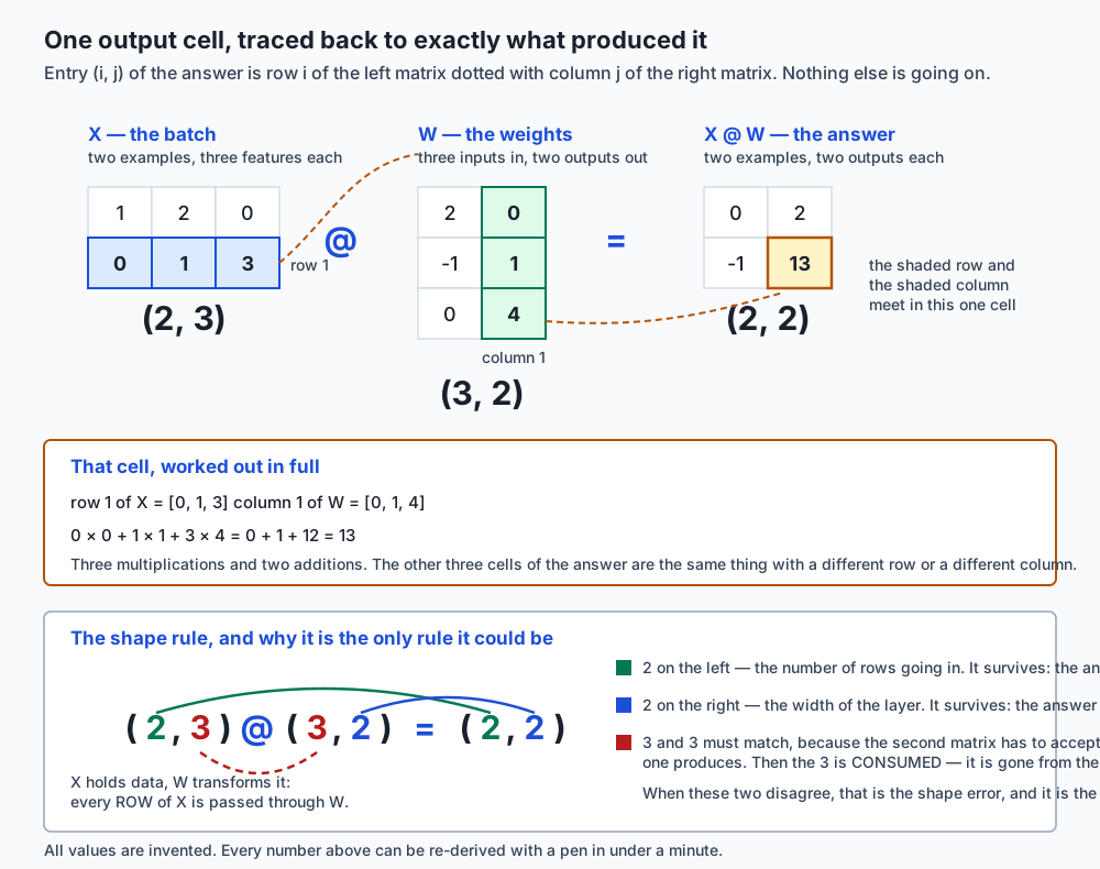
The shape rule, derived
(m, n) @ (n, p) -> (m, p)The two inner numbers must be equal. The two outer numbers survive. People memorise this and then check it nervously every time. Do not memorise it; read it off the machines.
A @ B means “do B, then do A”. B has shape (n, p): it accepts vectors of length p and produces vectors of length n. A has shape (m, n): it accepts vectors of length n and produces vectors of length m. So:
- The inner dimensions must match because A has to accept what B hands it. If B produces length-
nthings and A only takes length-kthings, you cannot bolt them together. - That inner dimension is then consumed. It does not appear in the answer at all. It was the size of the intermediate thing on the bench, and the combined machine has no bench.
- The outer dimensions survive because they are the two ends of the pipeline: what goes in at one end and what comes out at the other.
What it is not
| It is not | Why people think it is | What is actually true |
|---|---|---|
| Entry-by-entry multiplication | It is what “multiply” means for ordinary numbers, and NumPy’s * does exactly this | * is the elementwise or Hadamard product. It is a different operation with different uses. @ sums; * does not. |
| Commutative | Multiplication of numbers is, and the notation looks the same | A @ B and B @ A are usually different matrices, and are frequently not even the same shape. Often only one of them is legal at all. |
| Just a table lookup rule | It is taught as a recipe | It is composition of transformations. The recipe is the coordinate form of that. |
| Expensive because it is complicated | The formula looks fussy | It is expensive because there are m × n × p multiplications, not because any one of them is hard. |
The same thing as np.dot | They agree on 2-D arrays | They agree on 2-D arrays and diverge on higher-dimensional ones, as shown below. |
Why it was created and what problems it solves
Cayley defined this operation to solve a specific problem: he had two linear substitutions — rules that rewrite one set of variables in terms of another — and he wanted to know what happens when you apply one after the other. The answer is another linear substitution, and its coefficients turn out to be exactly the row-times-column combination of the original two. He named that combination the product, and the notation has not changed since.
The problem it solves for you is the same problem in modern clothes: you have a pipeline of transformations, and you want to collapse it into one.
That sounds abstract until you notice how much of computing is exactly that.
Graphics. A model in a 3-D scene gets rotated, scaled, moved, and projected onto your screen. Each of those is a matrix. Rather than pushing every one of a million vertices through five transformations, you multiply the five matrices together once and push each vertex through the single result. Five million operations become one million plus a fixed cost, and this is why real-time 3-D graphics is possible at all.
Neural networks. A layer transforms a batch of examples. Stacking layers is composing transformations. The entire forward pass of a model is a chain of matrix products with non-linear functions wedged between them — and today’s lab shows what happens when you leave those non-linear functions out, which is that the whole stack collapses back into a single matrix. That collapse is the reason activation functions exist, and it is a direct consequence of associativity.
Solving equations. Writing a system of linear equations as A @ x = b turns “many equations in many unknowns” into a single statement about one transformation, and lets you ask “what did this machine do to my input?” rather than juggling coefficients.
Graphs. If A is a table saying which nodes connect to which, then A @ A counts paths of length two, and A @ A @ A counts paths of length three. That is not an analogy — it falls straight out of the definition, because the sum over the middle index is exactly “count every way to get from here to there via somewhere”.
Probability. If M holds the probabilities of moving between states in one step, M @ M holds them for two steps. Same mechanism.
The common thread is that in every one of these, the useful thing is not the numbers in the matrix but the fact that composing is itself an operation you can compute. If composition were not a matrix, you could not precompute it, and nearly all of the above would be impractical.
How it works
Composition, with real coordinates
Take two transformations of the flat plane, both simple enough to picture.
A = [[0, -1],        a quarter turn anticlockwise
     [1,  0]]

B = [[1,  0],        a reflection in the horizontal axis
     [0, -1]]
Check those against the trick from earlier. A’s columns are [0, 1] and [-1, 0], so A sends (1, 0) to (0, 1) and sends (0, 1) to (-1, 0) — which is exactly a quarter turn anticlockwise. B’s columns are [1, 0] and [0, -1], so B leaves (1, 0) alone and flips (0, 1) to (0, -1) — a reflection that leaves x alone and flips y. No arithmetic required.
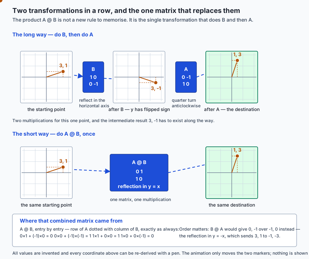
Now take the point v = (3, 1) and do B first, then A:
      B @ v          = [3, -1]      the reflection flipped the sign of y
      A @ (B @ v)    = [1, 3]       then the quarter turn
And now the product matrix, computed with the ordinary recipe:
      A @ B          = [[0, 1], [1, 0]]
      (A @ B) @ v    = [1, 3]
Same destination. One multiplication instead of two, and no intermediate (3, -1) on the bench. That block is captured from 02_composition.py in today’s lab, which asserts every line of it.
The product [[0, 1], [1, 0]] is the matrix that swaps the two coordinates, which is the reflection in the line y = x — and (3, 1) becoming (1, 3) is visibly exactly that. So “reflect in the horizontal axis, then turn a quarter anticlockwise” is the same thing as “reflect in the diagonal”. That is a real geometric fact that you could have found with a mirror and a piece of paper, and the matrix product found it for you by arithmetic.
Read the order carefully, because this is the thing people get wrong
In A @ B, B runs first. It is the matrix standing next to the vector in A @ (B @ v).
Matrices compose right to left, like nested function calls: A(B(v)). English reads “A times B” left to right; the arithmetic does not. That mismatch is the single most common conceptual error on this topic, and it is worth saying out loud every time until it sticks.
There is an honest complication here, and today’s lab meets it head-on rather than hiding it, because you will hit it in the first framework you use. Everything above assumes a vector is a column. Every deep learning framework instead stores a batch with one example per row, and then the matrix goes on the right:
| Convention | A vector is | A layer is written | A chain reads |
|---|---|---|---|
| Column (textbooks, this section) | a column, shape (n, 1) | y = A @ v | right to left: B @ (A @ v) |
| Row (every framework you will use) | a row, shape (1, n) | y = x @ A | left to right: x @ A @ B |
Both compute the same thing; one is the transpose of the other. The lab checks that x @ W and W.T @ x give identical numbers. Frameworks chose rows because a batch is a stack of examples, and stacking them as rows means example i lives at X[i] — which is how every CSV file (Day 65) and database table (Day 85) you have met is already laid out. The cost of that choice is one moment of confusion, and you are having it now, deliberately, rather than at 2am.
Not commutative, computed in full
Both A @ B and B @ A are defined here, because both matrices are 2 by 2. They are not the same:
  A @ B = [[0, 1], [1, 0]]     reflection in the line y = x
  B @ A = [[0, -1], [-1, 0]]   reflection in the line y = -x
Feed (3, 1) through each and you land at (1, 3) one way and (-1, -3) the other. Not close. Not a rounding difference. A different place.
The untidier pair from the opening does the same thing without any geometric prettiness to lean on:
      P @ Q = [[19, 22], [43, 50]]
      Q @ P = [[23, 34], [31, 46]]
      P * Q = [[5, 12], [21, 32]]
Two matrices, three answers, and only one of them is what “multiply these matrices” means.
What is true: associativity and distributivity
Two things you are allowed to do:
(A @ B) @ C  =  A @ (B @ C)          associativity — brackets may move
A @ (B + D)  =  A @ B  +  A @ D      distributivity — it splits over addition
Note the precise claim of associativity: the brackets may move freely; the order may not. Those are different statements and confusing them is the usual mistake.
Associativity is not a curiosity for algebra exams. It is the only reason you are allowed to choose the cheaper way to evaluate a chain — and the choice is worth a great deal.
An (m, n) @ (n, p) costs m × n × p multiplications, one per (row, column, inner step). Nothing about that count is an estimate; it is how many times the innermost line of the loop runs. So for a chain of three:
  (10, 100) @ (100, 5) @ (5, 50)
      (AB)C  = 10*100*5 + 10*5*50
             = 5,000 + 2,500 = 7,500
      A(BC)  = 100*5*50 + 10*100*50
             = 25,000 + 50,000 = 75,000
      ratio  = 10x
Ten times the arithmetic for the identical answer, decided entirely by where you put the brackets. And on shapes people actually train:
  (1024, 4096) @ (4096, 8) @ (8, 4096)
      (AB)C  = 1024*4096*8 + 1024*8*4096
             = 33,554,432 + 33,554,432 = 67,108,864
      A(BC)  = 4096*8*4096 + 1024*4096*4096
             = 134,217,728 + 17,179,869,184 = 17,314,086,912
      ratio  = 258x
Those are the shapes of a low-rank adapter: a 4096-wide layer with a narrow 8-wide detour through one matrix and back out through another, applied to a batch of 1024. Multiplying the two small matrices together first builds a full 4096 by 4096 matrix and then hits the entire batch with it — 258 times the work, for exactly the same answer. Keeping the brackets on the left keeps the detour narrow. That cost gap is most of why adapters are cheap enough to be worth using, and it is nothing more exotic than associativity plus counting.
The identity matrix
The straight pipe. Ones on the main diagonal, zeros everywhere else:
identity(3) = [[1, 0, 0], [0, 1, 0], [0, 0, 1]]Apply it to a vector and you get the vector back, because the weighted-sum-of-columns picture picks out exactly one column per coordinate. Multiply any matrix by it and nothing happens:
  I2 @ X      = [[1, 2, 0], [0, 1, 3]]    (X unchanged)
  X  @ I3     = [[1, 2, 0], [0, 1, 3]]    (X unchanged)
Note the two different sizes in that captured block. X is (2, 3), so the identity that fits on its left is 2 by 2 and the one that fits on its right is 3 by 3. “The” identity matrix is really one per size, and the shape rule decides which.
* versus @, deliberately
This is the trap from the opening, and it comes in two flavours.
Flavour one: same shape, different numbers. Two square matrices of the same size give a same-sized answer either way, so no shape check can save you. Only the values differ, and nothing tells you which you got. This is the dangerous one.
Flavour two: different shapes. Take the batch X of shape (2, 3) and the vector u = [10, 2, 5] of shape (3,):
  X * u  -> shape (2, 3)  [[10, 4, 0], [0, 2, 15]]
             u is broadcast across both rows (Day 100), then multiplied
             entry by entry. Three numbers per row go in, three come out.
  X @ u  -> shape (2,)     [14, 17]
             each row is multiplied by u AND THEN SUMMED:
               row 0: 1*10 + 2*2 + 0*5 = 10 + 4 + 0  = 14
               row 1: 0*10 + 1*2 + 3*5 =  0 + 2 + 15 = 17
The summing is the entire difference. * keeps every product; @ adds them up and loses a dimension doing it. In fact you can state the relationship exactly as code — @ is * followed by a sum along the last axis, which the lab asserts:
(X * u).sum(axis=1) == X @ uThat collapse is what makes @ a transformation rather than a rescaling. It is also why @ can turn three features into one number, and * never can.
np.dot, np.matmul, and @
Three spellings. On two-dimensional arrays all three agree exactly, and @ is the one to use because it says at a glance which operation you meant.
They part company on higher-dimensional arrays, and this was checked rather than assumed while writing this lesson — the assumption would have been that they differ everywhere, and they do not:
      a stack of two 2x2 matrices, shape (2, 2, 2), times one 2x2:
        np.matmul -> (2, 2, 2)
        np.dot    -> (2, 2, 2)
        Here they agree, in shape AND in every value.

      the same stack times ANOTHER stack, (2, 2, 2) against (2, 2, 2):
        np.matmul -> (2, 2, 2)      two matrices, paired up
        np.dot    -> (2, 2, 2, 2)   every pairing, all four
matmul treats the leading axes as a stack of matrices and pairs them off; dot sums over the last axis of the left and the second-to-last of the right, keeping everything else, so it produces every combination. The rule to carry is simpler than the exceptions: use @ for matrix multiplication, and np.dot only for two plain vectors.
Reading a shape error
The most common error in applied linear algebra, and the first thing to check when anything goes wrong:
  X is (2, 3). X @ X asks for (2, 3) @ (2, 3).
  The inner dimensions are 3 and 2, and they disagree.

  NumPy raises:
    ValueError: matmul: Input operand 1 has a mismatch in its core dimension 0,
    with gufunc signature (n?,k),(k,m?)->(n?,m?) (size 2 is different from 3)
Ignore the gufunc signature the first time you read it. Print the two shapes and look at the inner two numbers. That is the bug, and it is the whole bug.
The repair is usually a transpose — but there are two of them and they are not interchangeable:
  X @ X.T  is (2, 3) @ (3, 2) -> (2, 2)
      [[5, 2], [2, 10]]
      entry (i, j) is example i dotted with example j — a table of how
      alike the two EXAMPLES are.
  X.T @ X  is (3, 2) @ (2, 3) -> (3, 3)
      [[1, 2, 0], [2, 5, 3], [0, 3, 9]]
      entry (i, j) is feature i dotted with feature j — a table of how
      alike the three FEATURES are.
Both make the exception go away. Only one answers the question you had. This is why “just transpose it until it runs” is a genuinely bad habit: the error was telling you something, and silencing it at random trades a loud failure for a quiet wrong answer. Decide which table you wanted, then write that.
(Both results are symmetric, which ties back to Day 100 — a table of how alike two things are must read the same both ways round.)
An everyday analogy
Return to the machines, and let us push the analogy until it breaks, because an analogy you have not tested is one you will over-trust.
You run a small workshop. You have a cutting machine and a painting machine. Raw board goes into the cutter and comes out as shaped pieces; shaped pieces go into the painter and come out finished.
- A matrix is one machine. It has an input slot of a certain size and an output chute of a certain size. Those two sizes are the shape.
- The matrix product is welding two machines into one.
paint @ cutis the single unit that takes raw board in one end and finished pieces out the other. - The shape rule is the physical fit. The cutter’s output chute must fit the painter’s input slot. If it does not, you cannot weld them, and this is not a matter of opinion — it is the
ValueError. - The consumed inner dimension is the bench. When the machines are separate, shaped-but-unpainted pieces pile up between them. When you weld them, that pile stops existing. The intermediate size vanishes from the description of the combined machine, exactly as
nvanishes from(m, n) @ (n, p) -> (m, p). - Non-commutativity is obvious here. Cutting then painting gives finished pieces. Painting then cutting gives pieces with raw, unpainted edges. Same two machines, different factory, and nobody needs convincing.
- The identity matrix is a length of plain conveyor. Weld it on anywhere and nothing changes.
- Associativity is how you build the line. Weld the cutter to the painter first and then attach the sander, or weld the painter to the sander first and then put the cutter in front — either way the finished line is identical. The order of the machines along the line has not changed; only the order in which you did the welding.
- The multiplication count is the running cost. Welding does not make the work vanish. Every board still gets cut and painted. What welding saves is the handling: the bench, the pile, the carrying.
And now where the analogy breaks, which is the part worth stating:
A real welded machine does the same physical work as the two separate ones. A matrix product genuinely does less arithmetic per input than applying two matrices in turn — that is the whole point of precomputing it — but it costs something up front to build. For one vector, composing first is a waste. For a million vertices, it is the difference between a game that runs and one that does not. The analogy hides that trade-off, so hold it separately: compose once, apply many times.
The second break: machines are physical and a bench is a real place. The intermediate vector in A @ (B @ v) is real too, but the intermediate matrix in an association choice is not something anyone wants — as the 258× example showed, building the big intermediate matrix is precisely the expensive mistake. The analogy suggests bigger welded units are always better. They are not.
Examples in practice
One layer of a neural network. The payoff promised at the top. Here is the whole thing, with numbers you can check on paper.
X    = [[1, 2, 0],      the batch: two examples, three features each
        [0, 1, 3]]

W    = [[ 2, 0],        the weights: three inputs, two outputs
        [-1, 1],
        [ 0, 4]]

bias = [5, -2]          one number per OUTPUT unit
The multiply, worked out:
  example 0 = [1, 2, 0]
    output 0, weights [2, -1, 0]:  1*2 + 2*(-1) + 0*0  =  2 - 2 + 0  =  0
    output 1, weights [0,  1, 4]:  1*0 + 2*1    + 0*4  =  0 + 2 + 0  =  2
  example 1 = [0, 1, 3]
    output 0, weights [2, -1, 0]:  0*2 + 1*(-1) + 3*0  =  0 - 1 + 0  = -1
    output 1, weights [0,  1, 4]:  0*0 + 1*1    + 3*4  =  0 + 1 + 12 = 13
Then the bias, broadcast across the rows exactly as Day 100 described — (2, 2) against (2,) pads to (1, 2), the trailing 2s match, and the 1 stretches down the rows:
    example 0: [ 0,  2] + [5, -2] = [5,  0]
    example 1: [-1, 13] + [5, -2] = [4, 11]

  X @ W + b = [[5, 0], [4, 11]]   shape (2, 2)
That is a forward pass. Every model you will ever train is that operation, repeated at larger sizes, with a non-linear function applied between layers.
Three details in it are worth naming. The bias is one per output, not one per example — grow the batch to 64 and the bias does not change, because it belongs to the layer. Each row is computed independently of the others, which is exactly why batching is worth doing: the same weights get reused across every example in one multiply. And the 3 disappeared: three features went in, two outputs came out, and the width of the layer decided the shape of the answer.
Two layers, and why activation functions exist. Stack a second layer on top and the shapes chain: 3 features in, 2 hidden, 3 out. But the lab shows something uncomfortable:
      W @ W2 has shape (3, 3), and X @ (W @ W2) + (b @ W2 + b2) =
      [[5, 1, 9], [37, 12, 7]]
      — identical to running the two layers separately.
Two layers with nothing between them collapse into one matrix. That is associativity, and it means a stack of pure matrix multiplies is just one matrix multiply, no matter how deep you make it. Depth buys you nothing without a non-linear function in between. That is not a design preference; it is a theorem, and you have just seen it demonstrated on numbers you can check.
Graphics. A rotation, a scale and a translation, multiplied into one matrix and applied to every vertex of a model.
Recommendations. A matrix of users by features multiplied by a matrix of features by items gives a table of predicted scores — every user against every item, in one operation.
Attention. The mechanism behind every transformer model computes Q @ K.T — a table of how much each token should attend to each other token. That is a matrix product, and it is the same “table of how alike two things are” you saw in X @ X.T above, at a larger size.
Implications: security, privacy, performance, scalability, and cost
Performance is the headline, and there is a genuine surprise in it. Today’s lab times three nested Python loops against NumPy on two 200 by 200 matrices — eight million multiply-and-adds either way, and identical answers. Measured on the authoring machine (macOS 26.5.2, Apple Silicon, Python 3.14.0, NumPy 2.5.2):
      three nested loops in Python  :    0.1957 s
      NumPy @ on int64  (best of 5) :  0.002479 s          79x faster than the loop
      NumPy @ on float64 (best of 5):  0.000037 s       5,223x faster than the loop
Read the last two lines again. Same shapes, same values, same operator, same library — and the float version was 66 times faster than the integer version. That was not what this lesson expected to find, and it is the most instructive number in the day, because it tells you what NumPy is actually doing.
BLAS implements floating point and nothing else. Its matrix-multiply routines are defined for float and complex types. So a float64 multiply is handed straight out to BLAS — compiled, tuned to the exact processor, using vector instructions and cache-aware blocking and often several cores — while an int64 multiply falls back to NumPy’s own compiled C loop. Still far better than interpreted Python, still nowhere near BLAS.
Which means the usual answer to “why is NumPy fast?” — because it is C — is wrong. The int64 row is C, and it is the slow NumPy row. NumPy is fast because for the types that matter it stops being NumPy too, and calls out to a library people have been optimising since 1979. (This installation reported its BLAS as accelerate, read from numpy.__config__ rather than assumed; a Linux wheel will usually report OpenBLAS.)
The practical rule: if a matrix multiply is slower than you expected, check the dtype before you check anything else. It is also part of why every framework stores weights as float32 or something smaller, never as integers.
Those durations are from one machine on one day and yours will differ. No test in the lab asserts a duration; the assertions are wide ratios set far below what was measured.
Scalability is cubic, and that is unforgiving. An (n, n) @ (n, n) costs n³ multiplications. Double the size, do eight times the work. A 200 by 200 pair is eight million operations; a 1000 by 1000 pair is a billion. Nothing warns you, no exception is raised, and the process simply does not come back. This is the one resource in today’s lab that can genuinely make your machine uncomfortable, and the remedy is to raise sizes by doubling rather than jumping to a round number.
Cost, in money. Training compute is dominated by these products, so the multiplication count is the bill. This is why the association-order choice in the adapter example matters: 258× the arithmetic is 258× the energy and, near enough, 258× the rental cost of the machine doing it. Choosing where to put the brackets is one of the few optimisations that is free, exact and requires no approximation whatsoever.
Numerical honesty, which is the security-flavoured part. Two facts from the lab, both verified by running rather than by reasoning:
Integer matrix products overflow silently. NumPy integer arrays are fixed-width and wrap round; Python’s own integers are arbitrary-precision and do not. So the from-scratch implementation and NumPy genuinely disagree on large values, and NumPy is the one that is wrong:
big = [[3037000500, 0], [0, 1]]
np.array(big) @ np.array(big)   ->  [[-9223372036709301616, 0], [0, 1]]
matmul_loops(big, big)          ->  [[ 9223372037000250000, 0], [0, 1]]
3037000500 ** 2                 ==    9223372037000250000
No warning is raised. The array simply contains a large negative number where a large positive one belongs. The lab asserts this, including the absence of a warning, so the claim stays honest if NumPy ever changes.
Floating-point addition is not associative. With float64 inputs, (A @ B) @ C and A @ (B @ C) agree to within 1e-9 but are not bit-for-bit identical, even though they are the same computation in mathematics. Never compare two float results with ==; state a tolerance. Day 70 covered why.
Privacy. A trained weight matrix is not anonymous. W is derived from the data it was trained on, and matrix products are invertible often enough that “we only shipped the weights, not the data” is a weaker claim than it sounds. That is well beyond today’s scope, but it is the right instinct to form now.
Alternatives: free, open source, and commercial
Every option below is free and open source. Only the first two were actually run for this lesson; the rest are described from their own documentation, and no output is reproduced for them.
Pure Python lists and loops — run here. Free, no install, standard library only. When to choose it: when you are learning, when you need arbitrary-precision integers that do not overflow, or when there is genuinely no dependency available. How: three nested loops, as in the lab’s matmul_loops. Example: the entire from-scratch build in today’s exercise 1, which needs nothing but python3. The catch: measured at roughly 5,200 times slower than NumPy on 200 by 200 floats on this machine.
NumPy — run here, version 2.5.2. Free, BSD 3-Clause licence. When to choose it: essentially always, for array work on a single CPU. It is the foundation almost everything else in the Python numerical stack is built on. How: A @ B. Example: every captured block in this lesson. The catch: CPU only, no automatic differentiation, and — as measured above — the dtype decides whether you reach BLAS at all.
PyTorch — not installed, no output reproduced. Free, open source. When to choose it: when you need the same operation on a GPU, or you need gradients computed automatically for training. Its tensors deliberately mirror NumPy’s interface, and @ works the same way, which is much of why NumPy is worth learning first. How, from its documentation: torch.matmul(a, b) or a @ b, with .to("cuda") to move the data to a GPU. Cost: free; the GPU it wants to run on is the expense.
JAX — not installed, no output reproduced. Free, open source. When to choose it: when you want NumPy’s interface with just-in-time compilation and automatic differentiation, particularly for research code. How, from its documentation: jax.numpy mirrors the NumPy interface, so a @ b again, with jax.jit to compile a whole function. Cost: free.
BLAS implementations generally — present here but not chosen. OpenBLAS, Intel MKL, Apple’s Accelerate, and others. This is the honest and slightly surprising entry in the list: you are already using one. NumPy does not implement floating-point matrix multiplication itself; it calls out to whichever BLAS it was built against, which is why the loop loses so badly and why the int64 row above is so much slower than the float64 one. When to choose one deliberately: rarely, and only if you are building NumPy yourself or profiling has shown BLAS to be your bottleneck. How to see yours: numpy.__config__.show(). Cost: free for OpenBLAS and Accelerate; MKL is free to use with its own licence terms.
The practical recommendation: learn it with loops, use NumPy, reach for PyTorch or JAX when you need a GPU or gradients. The operation is identical in all of them, which is the point — you are learning one thing, not four.
Comparison with related concepts
| Operation | Notation | What it does | Result shape from (2, 3) and… | Sums? |
|---|---|---|---|---|
| Matrix product | A @ B | Composition of transformations | (3, 2) gives (2, 2) | Yes |
| Elementwise (Hadamard) product | A * B | Multiplies matching entries | (2, 3) gives (2, 3) | No |
| Dot product | u · v | Two vectors to one number | two (3,) vectors give a scalar | Yes |
| Matrix-vector product | A @ v | Weighted sum of A’s columns | (3,) gives (2,) | Yes |
| Scalar multiplication | 3 * A | Scales every entry | gives (2, 3) | No |
| Matrix addition | A + B | Adds matching entries | (2, 3) gives (2, 3) | No |
| Transpose | A.T | Swaps rows and columns | gives (3, 2) | No |
| Outer product | np.outer(u, v) | Every pairing of two vectors | (2,) and (3,) give (2, 3) | No |
Two comparisons deserve a sentence each.
Elementwise versus matrix product is the distinction this whole lesson keeps returning to, and the compact statement is: A @ B is A * B-style multiplication followed by a sum, arranged so that each output entry pairs one row with one column. The sum is the difference, and the sum is what loses a dimension.
Outer product versus dot product are opposites worth knowing as a pair. The dot product takes two vectors and returns one number — it collapses. The outer product takes the same two vectors and returns a whole matrix of every pairwise product — it expands. Both are matrix products in disguise: u · v is (1, n) @ (n, 1) giving (1, 1), and the outer product is (n, 1) @ (1, m) giving (n, m). Same operation, opposite arrangements, which is a nice demonstration that the shape rule really is doing all the work.
When to use it — and when not to
Use a matrix product when you are composing transformations, applying one transformation to many vectors at once, or computing every pairwise combination of two sets of things — similarity tables, attention scores, path counts in a graph.
Precompute the product when you will apply the same chain of transformations many times. Compose once, apply many. For a single vector it is a waste; for a million vertices it is the difference between working and not.
Do not use it when you want entry-by-entry arithmetic. If you are scaling each feature by its own factor, masking values, or applying a gate, you want *. Reaching for @ there is not a slower way to get the answer; it is a different and wrong answer.
Do not use it when the operation is not actually linear. Matrix multiplication can only express transformations where scaling the input scales the output and adding inputs adds outputs. Anything else — a threshold, a maximum, a comparison — is not a matrix and cannot be made into one. This is exactly why activation functions sit between layers rather than being folded into them.
Watch the association order when a chain has a narrow matrix in it. That is where the 258× lives, and it costs nothing to check.
Watch the dtype when speed matters. Integers do not reach BLAS.
Stop and think when you find yourself adding a transpose to make an error go away. The error was information. Work out which of the two possible repairs answers your question before you pick one.
Where this goes next in AI work
Day 102 takes the transformation reading further into linear transformations proper. But the thread that runs straight from today into everything else is this: a GPU is, for these purposes, a machine built to do this one operation in parallel.
Day 2 raised the question of why GPUs beat CPUs at bulk mathematics, and now you can answer it precisely rather than vaguely. Every entry of a matrix product is independent of every other entry — entry (0, 0) does not need to wait for entry (0, 1), because they read different rows and columns and write different places. A CPU has a handful of very fast cores designed to run complicated, branchy, unpredictable code. A GPU has thousands of simpler cores designed to run the same instruction over enormous amounts of data at once. Matrix multiplication is the purest possible case of that pattern: millions of identical multiply-and-add operations with no dependencies between them.
That is the whole answer. GPUs are not generally faster than CPUs — they are dramatically slower at most things. They are faster at this, and this is what training a model consists of. Modern accelerators have gone further and added units that do nothing but small matrix multiplies in a single instruction, which is as literal a statement of the point as hardware can make.
So when you read that a model took a certain number of GPU-hours to train, you are reading a count of these products. When someone quantises a model to run in fewer bits, they are making these products cheaper. When an adapter trains a large model at small cost, it is the association trick from earlier. Today’s operation is not one topic among many in AI. It is the operation, and almost everything else is arranged around making it fast enough.
Knowledge check
Eight questions on this lesson are provided in quiz.yml and rendered with the lesson. Before you take them, check yourself on the six things that matter most:
- Why must the inner dimensions match? (Answer in terms of what each matrix accepts and produces, not “because that is the rule”.)
- What is
A @ v, described as something done to A’s columns? - In
A @ B @ v, which matrix meets the vector first? - What is the one-sentence difference between
*and@? - Two associations of a three-matrix chain: do they give the same answer, and do they cost the same?
- Why is
float64matrix multiplication so much faster thanint64in NumPy?
Hands-on exercise
Today’s lab is “Multiply It Yourself”, in labs/sections/math-statistics-and-data/day-101-matrix-multiplication/.
You will implement matrix multiplication three different ways from first principles — three nested loops, a list of dot products, and a weighted sum of columns — and assert all three against NumPy’s @ on six shapes. Then you verify one output cell by hand, demonstrate that A @ B and B @ A differ, prove that * and @ are different operations on the same operands, trigger a shape error deliberately and repair it with a transpose, compute one network layer with a broadcast bias, and time your loop against NumPy.
Set up, from the repository root:
cd labs/sections/math-statistics-and-data/day-101-matrix-multiplication
python3 -m venv .venv
.venv/bin/pip install -r requirements/requirements.txt
Read starter/00_brief.md, then work through the six exercises, checking yourself as you go:
.venv/bin/pytest starter -qWrite your predictions down before you run anything. Every prediction in answers.py takes under a minute with a pen, and a prediction you check is worth ten outputs you read.
Expected output
On an untouched checkout the starter suite reports:
1 passed, 56 skippedA skip means “not attempted”. A failure means “attempted and wrong”, and prints both your answer and the real one. When it prints 57 passed, you are finished.
The reference suite and the full harness:
71 passed
58 checks, 0 failure(s).
Blocks worth recognising when you meet them. The highlighted output cell:
      row 1 of X    = [0, 1, 3]
      column 1 of W = [0, 1, 4]
      0*0 + 1*1 + 3*4 = 0 + 1 + 12 = 13
Composition arriving at the same point two ways:
      B @ v          = [3, -1]      (reflected: y flipped sign)
      A @ (B @ v)    = [1, 3]      (then turned a quarter anticlockwise)
      A @ B          = [[0, 1], [1, 0]]
      (A @ B) @ v    = [1, 3]
And the timing, whose ratios are the point and whose durations are not:
      three nested loops in Python  :    0.1957 s
      NumPy @ on int64  (best of 5) :  0.002479 s          79x faster than the loop
      NumPy @ on float64 (best of 5):  0.000037 s       5,223x faster than the loop
expected-output/FIELDS.md records exactly which parts of the captured output may legitimately differ on your machine and which may not.
Validate your work
bash tests/run_tests.sh; echo "exit=$?"prints58 checks, 0 failure(s).andexit=0..venv/bin/pytest examples -q -p no:cacheproviderprints71 passed..venv/bin/pytest starter -q -p no:cacheproviderprints57 passedonce you have finished.- Each of the five reference scripts ends with
every assertion held. find . -type d -name '__pycache__' -o -type d -name '.pytest_cache'prints nothing after a full run.
Troubleshooting
ModuleNotFoundError: No module named 'matmul' — you are running a reference script from the wrong directory. They import from beside themselves, so cd examples first.
Everything in the starter suite shows as s — that is correct on an untouched checkout. s means skipped, which here means “not attempted”. Run with -rs to see the reason for each one.
ValueError: matmul: Input operand 1 has a mismatch in its core dimension 0 — the shape error. Print both shapes and look only at the inner two numbers.
TypeError: unsupported operand type(s) for @ — you are using @ on plain Python lists. Convert with np.array(...) first, or call your own matmul_loops.
Your timings look nothing like the captured ones — expected, and fine. No test asserts a duration. But if your float64 result is not much faster than your int64 result, that is worth investigating: it suggests your NumPy is not reaching BLAS.
The lab’s troubleshooting.md covers all of these in more detail, plus the module-name collision between the two directories that was found while building the previous day’s lab.
Common mistakes
Building the result grid with [[0] * p] * m. It looks equivalent to the comprehension and is a bug: it makes m references to one row, so writing to C[0][0] changes every row at once. This is Day 100’s view-versus-copy lesson appearing in plain Python with no NumPy involved. There is a test that catches it and says so by name.
Getting the composition order backwards. In A @ B, B runs first. English reads left to right and the arithmetic does not.
Writing matvec as “dot with each row”. It gives the right numbers and the wrong picture, and the picture is what you came for. Write it as a weighted sum of columns.
Transposing until the error goes away. X @ X.T and X.T @ X are both legal, have different shapes, and answer different questions. Decide which one you meant.
Reaching for @ when you wanted *. If you are scaling each feature by its own factor, you want elementwise. @ will sum your features together, which is a different and wrong answer that will not raise.
Filling in answers.py after running the code. Every prediction will be right and you will have learned nothing.
Practice assignment
Build a tiny two-layer network by hand and in code, and prove the two agree.
- Invent a batch
Xof shape(3, 4)— three examples, four features — using small integers you can compute with. - Invent
W1of shape(4, 3)and a biasb1of shape(3,); thenW2of shape(3, 2)and a biasb2of shape(2,). - On paper, compute
H = X @ W1 + b1, thenY = H @ W2 + b2. Show your working for at least two cells in full, in the style used throughout this lesson. - Now write it in NumPy and assert your hand-computed
Ymatches, entry for entry. - Count the multiplications each layer costs, and state the total.
- Collapse the two layers into one: compute
W_combined = W1 @ W2andb_combined = b1 @ W2 + b2, and assert thatX @ W_combined + b_combinedequalsY. Then write two sentences explaining what this proves about depth without activation functions. - Finally, apply a non-linear function between the layers —
H_relu = np.maximum(H, 0)is enough — and show that the collapse no longer works. This is the single most important thing in the assignment.
Write it as one script that prints its working and asserts every claim, in the style of the lab’s reference scripts. If an assertion fails, the script should stop rather than print something reassuring.
Extension challenge
Pick one. Each is a genuine investigation with a real answer, not a busywork exercise.
1. Find the crossover. matmul_loops beats NumPy at some very small size, because NumPy has a fixed per-call overhead that the loop does not pay. Find that size on your machine by doubling. Then find out whether the crossover moves when you switch the arrays between int64 and float64, and explain why using what this lesson said about BLAS.
2. Optimal chain order. Given shapes [(10, 100), (100, 5), (5, 50), (50, 2)], write a function that tries every possible bracketing and returns the cheapest along with its multiplication count. Four matrices have five bracketings; six have forty-two. Look up how fast that count grows before you try ten — and then look up “matrix chain multiplication” to find the dynamic-programming solution that makes it tractable.
3. Strassen’s algorithm. Implement the 1969 method for the 2 by 2 case: seven multiplications instead of eight. Check it against your own matmul_loops on random inputs. Then write a paragraph on why a 12.5% saving in multiplication count does not translate into a 12.5% speedup in practice — the answer involves additions, cache behaviour, and numerical stability, and finding it is the point of the exercise.
4. The backward pass. If a layer computes Y = X @ W, the gradient flowing back to X is G @ W.T and the gradient for W is X.T @ G, where G has the shape of Y. Do not take that on trust: check that the shapes work out for the X and W in this lesson, and notice that both transposes you met when repairing the shape error have now turned up doing real work. Then explain, in terms of the shape rule alone, why those are the only two arrangements that could possibly have been correct.
5. High-dimensional angles. Using the geometric form of the dot product, write a function returning the angle between two vectors in degrees. Verify it gives exactly 45° for [2, 0] and [1, 1] and exactly 90° for [3, 4] and [-4, 3]. Then generate a thousand pairs of random vectors in 300 dimensions and plot the distribution of angles between them. The result is genuinely surprising, and it explains a great deal about how embeddings behave.
Quiz
Q1. A has shape (2, 3) and B has shape (3, 4). Why must those inner dimensions — the 3 and the 3 — be equal?
- So that the answer comes out square, which matrix multiplication requires
- Because A @ B means do B and then do A, and A can only accept vectors of the length B produces
- It is a convention chosen to make the arithmetic tidy; other definitions are equally valid
- Because both matrices must contain the same number of entries in total
Show answer
Answer: B. Because A @ B means do B and then do A, and A can only accept vectors of the length B produces
Read the shapes as machines. B is (3, 4), so it accepts vectors of length 4 and produces vectors of length 3. A is (2, 3), so it accepts vectors of length 3 and produces vectors of length 2. The inner dimensions must match because the second thing has to accept what the first one hands it — that is the whole reason, and it is why the rule is not something you need to memorise. Notice too what happens to that 3: it is CONSUMED. It was the size of the intermediate result, and the combined transformation has no intermediate, so it does not appear in the answer (2, 4) at all. Option 0 is simply false — the answer here is (2, 4), which is not square, and most useful products are not. Option 2 gets the history backwards: Cayley defined the product in 1858 precisely because it was the operation that composed two linear substitutions, so composition came first and the recipe is what you get by writing it out in coordinates. Option 3 is not a rule of anything: A has 6 entries here and B has 12.
Q2. P and Q are both (2, 2). Which statement about `P * Q` and `P @ Q` in NumPy is true?
- `*` raises a ValueError, because matrices must be multiplied with `@`
- They return arrays of different shapes, so a shape check will catch the mistake
- Both are legal, both return a (2, 2) array, and the values are completely different
- They are the same operation; `@` is simply the newer spelling of `*`
Show answer
Answer: C. Both are legal, both return a (2, 2) array, and the values are completely different
This is the trap the lesson opens with, and it is dangerous precisely because nothing goes wrong visibly. With P = [[1, 2], [3, 4]] and Q = [[5, 6], [7, 8]], P * Q is [[5, 12], [21, 32]] — every entry multiplied by the matching entry, nothing summed — while P @ Q is [[19, 22], [43, 50]], each entry a row dotted with a column. Both are (2, 2). No exception, no warning, not one number in common. Option 1 describes the safer case, which happens only when the shapes are such that one of the two operations is illegal; on two square matrices of the same size you get no such protection. The one-sentence statement worth carrying is that `@` is `*` followed by a sum along the last axis — the summing is the entire difference, and it is what loses a dimension and makes the result a transformation rather than a rescaling.
Q3. A is a quarter turn anticlockwise and B is a reflection in the horizontal axis. In `A @ B @ v`, which transformation is applied to v first?
- B, because the rightmost matrix is the one standing next to the vector
- A, because expressions are read left to right
- They are applied simultaneously, so the question does not arise
- It depends on whether A and B commute
Show answer
Answer: A. B, because the rightmost matrix is the one standing next to the vector
Matrices compose right to left, exactly like nested function calls: A @ B @ v is A(B(v)), and B is the one touching the vector. Working it through with v = (3, 1): B sends it to (3, -1) by flipping the sign of y, then A turns that a quarter anticlockwise to (1, 3). The single product A @ B is [[0, 1], [1, 0]], the reflection in the line y = x, and applying it to (3, 1) in one step also gives (1, 3) — same destination, one multiplication instead of two. Option 1 is the mistake almost everyone makes once, because English reads "A times B" left to right and the arithmetic does not. Option 3 is a real red herring: whether they commute affects whether the OTHER order gives the same answer, not which one runs first. Here they do not commute — B @ A is [[0, -1], [-1, 0]], the reflection in y = -x, which sends (3, 1) to (-1, -3) instead. One caveat worth carrying: all of this assumes vectors are columns. Frameworks store a batch with one example per row and write X @ W, where the chain then reads left to right — the same computation, transposed.
Q4. You have a chain (1024, 4096) @ (4096, 8) @ (8, 4096). What does the choice of bracketing change?
- The answer, because matrix multiplication is not associative
- Nothing measurable; both orders do essentially the same amount of work
- Only whether the operation is legal at all
- Nothing about the answer, but the arithmetic differs by a factor of 258
Show answer
Answer: D. Nothing about the answer, but the arithmetic differs by a factor of 258
Matrix multiplication IS associative, so both bracketings give the identical answer — that is a theorem, not a coincidence. What differs is the cost, and the gap is not a rounding difference. An (m, n) @ (n, p) costs m*n*p multiplications, so (AB)C costs 1024*4096*8 + 1024*8*4096 = 67,108,864, while A(BC) costs 4096*8*4096 + 1024*4096*4096 = 17,314,086,912. That is exactly 258 times more work for the same result, because multiplying the two small matrices together first builds a full 4096 by 4096 matrix and then hits the whole batch with it. Those are the shapes of a low-rank adapter, which people really do train, and this cost gap is most of why they are affordable. Option 0 confuses two different statements: the BRACKETS may move freely, the ORDER may not, and mixing those up is the usual mistake. Since training compute is dominated by these products, the multiplication count is effectively the bill — which makes bracket placement one of the very few optimisations that is free, exact and requires no approximation.
Q5. X has shape (2, 3), so `X @ X` raises a ValueError. Both `X @ X.T` and `X.T @ X` fix it. What should decide which one you write?
- Whichever one runs without raising — they compute the same thing either way
- X.T @ X always, since transposing the left operand is the conventional repair
- What the result means: one compares examples with examples, the other compares features with features
- Whichever produces the smaller array, to save memory
Show answer
Answer: C. What the result means: one compares examples with examples, the other compares features with features
They are not interchangeable and they are not the same size. X @ X.T is (2, 3) @ (3, 2) giving (2, 2), whose entry (i, j) is example i dotted with example j — a table of how alike the two EXAMPLES are, which for this X is [[5, 2], [2, 10]]. X.T @ X is (3, 2) @ (2, 3) giving (3, 3), whose entry (i, j) is feature i dotted with feature j — a table of how alike the three FEATURES are, which is [[1, 2, 0], [2, 5, 3], [0, 3, 9]]. Both are symmetric, as any such table must be. Option 0 is the habit worth breaking: "just transpose it until it runs" trades a loud failure for a quiet wrong answer, and the shape error was telling you something useful. Option 3 would have you pick on an irrelevance. The general discipline when a shape error appears is to print the two shapes, look only at the inner two numbers, work out which table you actually wanted, and then write that.
Q6. In NumPy, multiplying two 200 by 200 float64 arrays with `@` is dramatically faster than multiplying two int64 arrays of the same shape and the same values. Why?
- Floating-point numbers occupy less memory than 64-bit integers
- BLAS implements matrix multiply only for floating-point and complex types, so the integer case never reaches it
- NumPy checks every integer entry for overflow, and those checks dominate the time
- Integer arrays are stored as Python objects rather than as a contiguous block
Show answer
Answer: B. BLAS implements matrix multiply only for floating-point and complex types, so the integer case never reaches it
This was measured while writing the lesson rather than assumed, and it contradicted the expectation. On the authoring machine the same 200 by 200 product took 0.002479 s as int64 and 0.000037 s as float64 — the float version 66 times faster, with identical shapes, identical values and the identical operator. The reason is that NumPy does not implement floating-point matrix multiplication itself; it hands the work to BLAS, whose matrix-multiply routines are defined only for float and complex types. An int64 product therefore falls back to NumPy own compiled C loop — far better than interpreted Python, and nowhere near BLAS. This is why the usual answer to "why is NumPy fast?" — because it is C — is wrong: the int64 row IS C, and it is the slow NumPy row. Option 0 is false; both are 8 bytes here. Option 2 is false; NumPy integer arithmetic wraps silently with no checks at all, which is a separate hazard worth knowing. Option 3 describes a Python list, not a NumPy array. The practical rule: if a matrix multiply is slower than you expected, check the dtype before anything else.
Q7. A network layer computes `X @ W + b`, where X is (64, 3) — a batch of 64 examples — and W is (3, 2). What shape must b have?
- (64,), one bias per example in the batch
- (64, 2), a separate bias for every example and every output
- (2,), one bias per output unit
- (3,), one bias per input feature
Show answer
Answer: C. (2,), one bias per output unit
X @ W is (64, 3) @ (3, 2), which gives (64, 2). The bias has one entry per OUTPUT unit, so it is (2,), and broadcasting adds that same pair of numbers to every one of the 64 rows: lining (64, 2) up against (2,) pads to (1, 2), the trailing 2s match, and the 1 stretches down the rows. The test that settles it is to grow the batch — the bias belongs to the layer, not to the data, so going from 64 examples to 640 changes the shape of X and nothing else. That independence is exactly what makes batching worth doing: the same weights and the same bias are reused across every example in a single multiply, and each row is computed without reference to any other. Option 0 is the tempting wrong answer because 64 is the number you were just looking at. Getting this wrong does at least raise a ValueError naming both shapes rather than failing silently — one of the few places in this area where you are told.
Q8. You stack two layers with no activation function between them: first `X @ W1 + b1`, then that result `@ W2 + b2`. What have you built?
- A genuinely two-layer network, since two matrix multiplies are strictly more expressive than one
- Something that will raise a shape error, because layers cannot be chained directly
- A network that is harder to train but ultimately more capable
- Exactly one layer: the pair collapses into a single matrix and a single bias
Show answer
Answer: D. Exactly one layer: the pair collapses into a single matrix and a single bias
Associativity does something uncomfortable here. X @ (W1 @ W2) + (b1 @ W2 + b2) produces exactly the same numbers as running the two layers in turn — the lab asserts it entry for entry. So the two layers collapse into one matrix W1 @ W2 and one bias, and this holds however deep you make the stack: a chain of pure matrix multiplies is just one matrix multiply. Depth buys nothing without something non-linear in between. That is not a design preference or a rule of thumb; it is a theorem, and it is the reason activation functions exist and sit BETWEEN layers rather than being folded into them. It also draws the boundary of what this operation can express: matrix multiplication can only represent transformations where scaling the input scales the output and adding inputs adds outputs. Anything else — a threshold, a maximum, a comparison — is not a matrix and cannot be made into one. Adding a single ReLU between the two layers breaks the collapse immediately, which is worth demonstrating for yourself.
Glossary
- Dot product
- The operation that takes two vectors of the same length, multiplies them entry by entry, and adds up the products, returning a single number rather than a vector. Written u dot v. It has an equivalent geometric form, the product of the two lengths times the cosine of the angle between them, and the two forms give the same number — which is why a dot product of zero means the vectors are perpendicular, and why a vector dotted with itself is its squared length.
- Matrix product
- The operation written A @ B, whose entry (i, j) is row i of A dotted with column j of B. The recipe is the coordinate form of something simpler: A @ B is the single transformation that does B and then does A. Cayley defined it this way in 1858 precisely because it was the operation corresponding to composing two linear substitutions, so composition is the definition and the recipe is the consequence, not the other way round.
- Composition
- Doing one transformation and then another. The reason matrix multiplication has the rule it has. Because matrices compose like nested function calls, the rightmost matrix in A @ B @ v is the one that meets the vector first — English reads left to right and the arithmetic does not, which is the single most common conceptual error on this topic.
- Inner dimension
- In an (m, n) @ (n, p), the n that appears on both sides. It must match because the second transformation has to accept what the first one produces, and it is then CONSUMED — it does not appear in the answer at all. It was the size of the intermediate result, and the combined transformation has no intermediate. When the two inner dimensions disagree, that is the shape error.
- Shape rule
- An (m, n) @ (n, p) gives an (m, p). Worth deriving rather than memorising: the inner dimensions match because of what each side accepts and produces, and the outer dimensions survive because they are the two ends of the pipeline — what goes in at one end and what comes out at the other. Reading a shape error means printing both shapes and looking only at the inner two numbers.
- Commutative
- An operation where the order of the operands does not change the answer. Addition of numbers is commutative; matrix multiplication is NOT. A @ B and B @ A are usually different matrices and frequently not even the same shape, and often only one of them is legal. This is not a technicality to be apologised for: it is the honest consequence of composition, in the same way that putting on socks and then shoes differs from shoes and then socks.
- Associative
- An operation where the brackets may be moved without changing the answer: (A @ B) @ C equals A @ (B @ C). Matrix multiplication is associative. Note the precise claim — the BRACKETS may move freely, the ORDER may not, and confusing those two statements is the usual mistake. Associativity is what makes it legal to pick the cheaper evaluation order, which on realistic adapter shapes is worth a factor of 258 in arithmetic for an identical answer.
- Distributive
- The property that A @ (B + C) equals A @ B plus A @ C — matrix multiplication splits over addition. It is what allows a layer weight matrix to be decomposed into a base part and a small correction whose results are then added, which is half the reason low-rank adapters work.
- Identity matrix
- The square matrix with 1 on the main diagonal and 0 everywhere else. The transformation that does nothing: applied to a vector it returns that same vector, and multiplying any matrix by it changes nothing. It is really one matrix per size, and the shape rule decides which — a (2, 3) matrix takes a 2 by 2 identity on its left and a 3 by 3 identity on its right. numpy.eye(n) builds one.
- Elementwise product
- Multiplying two arrays of the same shape entry by entry, with no summing anywhere, written A * B in NumPy. A different operation from the matrix product and not a slower or sloppier version of it. The compact way to hold the distinction: @ is * followed by a sum along the last axis, and it is the summing that loses a dimension and makes the result a transformation rather than a rescaling.
- Hadamard product
- The formal name for the elementwise product, so called after Jacques Hadamard. Worth knowing because papers use the name and a small circle symbol for it where code uses a bare asterisk, and a reader who does not recognise the name can mistake it for the matrix product and misread the whole equation.
- Linear combination
- A weighted sum of a set of vectors — so many copies of the first, plus so many of the second, and so on. The key to matrix-vector multiplication: A @ v is a linear combination of A COLUMNS, with the entries of v as the weights. This picture explains at once why the output has as many entries as A has rows, why v must have one entry per column, and why the answer can never land outside the space A columns reach.
- Basis vector
- One of the vectors that is all zeros except a single 1, such as (1, 0) and (0, 1) in the plane. Feeding one into a matrix picks out exactly one column, so the columns of a transformation matrix ARE the images of the basis vectors. That lets you read a transformation matrix straight off a picture — work out where each basis vector lands and write those down as the columns — with no arithmetic at all.
- Forward pass
- Computing a network output from its input by running the data through each layer in turn. One layer of it is X @ W + b: a matrix multiply and a vector add, with the bias broadcast across the rows of the batch. This is not a simplification for teaching — it is the actual operation, and it is where essentially all the compute in training goes.
- Batch
- A stack of examples processed together, conventionally with one example per ROW so that example i lives at X[i], matching the layout of every CSV file and database table. Each row is computed independently of the others, which is exactly what makes batching worth doing: one multiply reuses the same weights across every example. Growing the batch changes the shape of X and nothing else — the weights and the bias belong to the layer.
- Bias
- A vector added to a layer output after the matrix multiply, with one entry per OUTPUT unit rather than per example. It is added to every row of the product by broadcasting, so a layer two units wide takes exactly two numbers however large the batch is. Getting its length wrong raises a broadcasting ValueError rather than failing silently, which is one of the few places in this area where you are told.
- BLAS
- Basic Linear Algebra Subprograms — a standard interface for vector and matrix routines, published from 1979 onwards, with many competing implementations such as OpenBLAS, Intel MKL and Apple Accelerate. NumPy does not implement floating-point matrix multiplication itself; it calls out to whichever BLAS it was built against. Critically, BLAS matrix-multiply routines exist only for floating-point and complex types, which is why an int64 product in NumPy is measurably far slower than a float64 one of the same shape and values — the integer case falls back to NumPy own compiled loop and never reaches BLAS at all.
- Multiplication count
- How many multiplications a product costs: m times n times p for an (m, n) @ (n, p), one per row, column and inner step. Not an estimate — it is exactly how many times the innermost line of the loop runs. Since training compute is dominated by these products, the multiplication count is effectively the bill, which is why choosing the cheaper association of a chain is a free and exact optimisation.
- Shape error
- The ValueError raised when the inner dimensions of a product disagree, and the most common error in applied linear algebra. NumPy message mentions a gufunc signature which can be ignored on first reading; the useful part is the phrase naming the two sizes. The repair is usually a transpose, but there are two of them — X @ X.T compares examples with examples and X.T @ X compares features with features — and they have different shapes and different meanings, so transposing until the error goes away trades a loud failure for a quiet wrong answer.
- Low-rank adapter
- A way of adjusting a large layer by inserting a narrow detour: a wide input passes through one small matrix down to a few dimensions and back out through another. Its cost depends entirely on the association order — keeping the brackets so the batch meets the narrow matrices first costs 67 million multiplications on typical shapes, while multiplying the two small matrices together first builds a full wide matrix and costs 17.3 billion for the identical answer, a factor of 258.
Sources and further reading
- NumPy documentation — NumPy Developers (accessed 2026-08-16)
- NumPy: the absolute basics for beginners — NumPy Developers (accessed 2026-08-16)
- Matrix multiplication — Wikipedia (accessed 2026-08-16)
- Dot product — Wikipedia (accessed 2026-08-16)
- Essence of linear algebra — 3Blue1Brown (accessed 2026-08-16)
- Linear Algebra, Spring 2010 (18.06) — MIT OpenCourseWare (accessed 2026-08-16)
Kept in this browser, no account needed. Your progress page turns the whole record into one link you can bookmark or open on another device.