Math, Statistics, and Data › Linear Algebra I: Vectors and Matrices › Day 102
Day 102: Linear Transformations

After this lesson you will be able to look at any 2 by 2 matrix and say what it does to the plane, because you will know the one fact the whole subject rests on: a matrix is a function, and its columns are where the basis vectors land. If you know where (1, 0) and (0, 1) go, you know where every vector goes, and you never need the picture again. You will state the two conditions that make a transformation linear, test both on a matrix where they hold and on a function that adds a constant where they fail, and see that the failure is exactly the constant — which is the honest reason a network layer keeps its bias separate as X @ W + b. You will derive scaling, reflection, shear and rotation rather than memorise them, including deriving the rotation matrix from the unit circle with cosine and sine defined from scratch. You will compose two transformations into one matrix, get the order right and know why it reads backwards. You will meet the determinant as a measured area rather than a formula, with a negative one that reports a flip and a zero one that reports a permanent collapse, and you will know when an inverse exists and what NumPy raises when it does not. And you will finish holding the thing this day exists for: a linear transformation always fixes the origin and always sends straight lines to straight lines, so a stack of twenty of them is one 2 by 2 matrix and can draw no curve at all. That is the concrete, measured reason activation functions are not optional.
Hands-on lab for this lesson
Lab files on GitHub: https://github.com/ai-roadmap-365/ai-roadmap-365.github.io/tree/main/labs/sections/math-statistics-and-data/day-102-linear-transformations
- Get the hands-on files. Clone the labs repository once (you can reuse this clone for every lesson). This works on macOS, Linux, and Windows (PowerShell or WSL):
git clone https://github.com/ai-roadmap-365/ai-roadmap-365.github.io.git cd ai-roadmap-365.github.io - Open this lesson's lab. Move into the directory for this specific day. Every lab lives at the same predictable path — section / subsection / week / day:
cd labs/sections/math-statistics-and-data/day-102-linear-transformations - Read the lab guide. Open `README.md` in that directory. It lists the exact commands, what each does, the expected output, and how to check your work — read it before running anything.
- Run it and check your work. Follow the README's "How to run" section: run the example first to see the finished result, then complete the numbered exercises in `starter/`, then run the tests. The tests pass (exit 0) only when your work is correct.
bash tests/run_tests.sh # or the test command named in the lab README
You can also open the lab as a local page (works offline, shows the file tree and expected output).
Learning objectives
By the end of this lesson you will be able to:
- Read a transformation matrix off the landing places of the two basis vectors, read the landings back off the columns, and say why a row is never a landing place
- State the two conditions that define a linear transformation — it preserves addition and it preserves scalar multiplication — and test both in code
- Demonstrate that adding a constant breaks both conditions, and quantify the failure as exactly b and exactly (s minus 1) times b
- Explain why every linear transformation fixes the origin, and use that as a one-second test for linearity
- Derive the scaling, reflection and shear matrices from where the basis vectors land, rather than recalling them
- Derive the rotation matrix from the unit circle, defining cosine, sine and the radian along the way
- Compose two transformations into a single matrix, and read a product right to left because the first step stands next to the vector
- Interpret the determinant geometrically as the signed area factor, and measure it rather than compute it
- Say what a negative determinant means for orientation and what a zero determinant means for information
- State when an inverse exists, write down the inverse of a shear and a scaling by reasoning, and name the exception numpy.linalg.inv raises on a singular matrix
- Explain rank in plain language as how many dimensions survive, and read it off a 2 by 2 matrix by eye
- Compare floats with a stated tolerance and justify the number, knowing that cos of pi over 2 is not 0.0
- Explain, and demonstrate, why no stack of linear layers can separate data that needs a curve — and why that is the reason activation functions exist
Prerequisites
- Day 99 — vectors: components, magnitude, and what an arrow with coordinates means
- Day 100 — matrices and their three readings. Today is the third reading, in full
- Day 101 — matrix multiplication as composition. Today supplies the geometry behind the order rule
- Day 70 — floating point, which is why every comparison in this lesson declares a tolerance
- Day 43 — python3 -m venv and installing a package with pip; the lab installs numpy and pytest into a lab-local environment
- Days 71 to 74 — pytest, which the lab uses for both the reference suite and the running score
- No mathematics beyond school arithmetic. Cosine, sine and the radian are defined from the unit circle where they first appear
Why this matters
Here is a model that cannot work, and the reason has nothing to do with your learning rate.
You have four data points. Two of them belong to class A and two to class B, and they are arranged like this:
    (0, 0) -> A          (1, 1) -> A
    (1, 0) -> B          (0, 1) -> B
Class A sits on one diagonal, class B on the other. Draw them on paper and try to separate them with a single straight line. It takes about ten seconds to convince yourself that you cannot.
So you do the obvious thing. One line is not enough, therefore use more layers. You stack twenty matrix multiplications, one after another, and you train. The loss goes down a little and then flattens. Accuracy sits at chance. You try a bigger learning rate, a smaller one, more layers, wider layers, a different initialisation. Nothing moves.
Here is why, from a real run in today’s lab. Twenty 2×2 matrices with pseudo-random entries, applied one at a time to a point, against the same twenty multiplied together first and applied once:
  twenty applications:      (-3.5017165700891133, -4.824470758326175)
  one combined matrix:      (-3.501716570089111, -4.824470758326172)
  the combined matrix is    [[-2.5255936621574815, 4.334502516447186], [-3.4796240129856693, 5.97183487309051]]
  largest relative difference: 6.341021624128209e-16
Twenty layers deep, and the whole stack is one 2×2 matrix. Depth bought nothing at all. Whatever a single matrix could not do, twenty of them cannot do either, because twenty of them are a single matrix. And a single matrix, as this lesson will show you by measuring rather than asserting, always leaves the origin exactly where it found it and always sends straight lines to straight lines. It cannot bend. It cannot curve. It cannot separate those four points.
That is the honest, concrete reason activation functions exist. Not “non-linearity adds expressive power”, which is a sentence you can nod at without understanding. The reason is that without something non-linear wedged between them, your layers slide together into one layer, and you can watch it happen in four lines of output.
Getting there requires one idea, and today is built entirely on it:
A matrix is a function, and its columns are where the basis vectors land.
Day 100 listed three ways to read a matrix — as a table, as a collection of vectors, as a transformation — and promised that the third reading would get its own day. Day 101 showed that multiplying matrices is composing those transformations. Today the transformation reading gets the full treatment, and by the end you will be able to look at four numbers and say what they do to the plane, what they do to area, whether they can be undone, and what they can never do at any depth.
There is also a much smaller, much more immediate payoff, and it arrives in about ten minutes: linear algebra stops being a list of formulas to memorise. You will not memorise the rotation matrix today. You will derive it, from a circle, in three lines, and you will be able to re-derive it in a year when you have forgotten it.
The idea in plain language
Pick up a sheet of graph paper. Now imagine it printed not on paper but on a sheet of stretchy fabric, with one drawing pin through the origin holding it to the table.
You may pull the fabric. You may pull it harder in one direction than another, tilt it, slide the top sideways while the bottom stays put, spin it round the pin, or flip it over entirely. What you may not do is crumple it, fold it, tear it, or push it around so the printed lines curve. When you are done, the printed grid lines must still be straight, still evenly spaced, and still parallel to their neighbours — and the pin must still be through the origin.
That is a linear transformation. Everything in this lesson is a consequence of those restrictions.
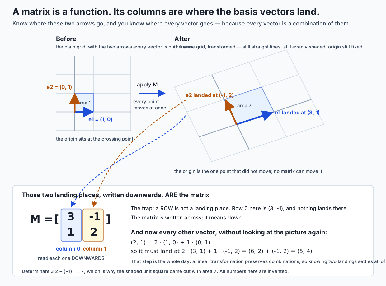
Now the useful part. Draw two arrows on the sheet before you stretch it: one arrow one unit to the right, and one arrow one unit up. Call them e1 and e2. They are the standard basis — the two arrows every other arrow on the sheet is built from, because “three right and two up” is just 3 · e1 + 2 · e2.
Stretch the sheet. Look at where those two arrows ended up.
That is all the information there is. Not “that is most of it” — that is all of it. Because the fabric had to keep its grid straight and evenly spaced, the point that was at (3, 2) had no choice about where to go: it was three e1 and two e2 before, so it is three of the new e1 and two of the new e2 now. Knowing two landing places settles every other landing place on the whole infinite sheet.
And a matrix is exactly the bookkeeping for those two landing places. Write the first landing down the left column, the second down the right column, and you have written the transformation down. Nothing else is in there.
Historical background
The honest version of this section is short, because only one date in it comes from a source this lesson cites.
Matrix multiplication — the operation that composes two of these transformations into one — “was first described by the French mathematician Jacques Philippe Marie Binet in 1812, to represent the composition of linear maps that are represented by matrices”. That is a direct quotation from the Wikipedia article on matrix multiplication listed in this lesson’s sources, and it is worth reading twice, because it settles a question of order that confuses people for years: matrix multiplication was not invented as an arithmetic operation that later turned out to be useful for transformations. It was invented to be composition of transformations. The row-by-column rule you were probably taught first is the consequence. The meaning came first.
That ordering explains the single most complained-about property of matrix multiplication, which the same article states plainly: it “is non-commutative, even when the product remains defined after changing the order of the factors”. Of course it is. Putting your socks on and then your shoes is not the same as putting your shoes on and then your socks. Composition of actions has never commuted, and nobody finds that strange until it is written with a multiplication sign.
Two things this lesson deliberately does not claim. First, the terminology: the Wikipedia article on linear maps, which this lesson also cites, gives the formal definition but carries no attribution for who introduced the concept or the term, so none is offered here. Inventing one would be easy and would be worthless. Second, the geometric teaching style: the idea of leading with “where do the basis vectors land” rather than with the row-by-column rule is most widely associated today with the Essence of linear algebra series listed in the sources, and with the geometric emphasis of MIT’s 18.06, also listed. Whether either of them originated the approach is not something the cited pages state, so this lesson does not say they did. It says only that they are where you should go next if today lands well.
Day 100 covered the longer history of the matrix as an object — from Chinese counting-rod methods through Cayley’s memoir. Today’s history is narrower and it is one sentence: the multiplication came from the composition.
What it is — and what it is not
A linear transformation is a function that takes a vector and returns a vector, subject to exactly two conditions. From the Wikipedia article on linear maps, the two conditions are:
Additivity: f(u + v) = f(u) + f(v)
Homogeneity: f(cu) = cf(u) where c is a scalar
That is the whole definition. Every geometric fact in this lesson — the pinned origin, the straight lines, the even spacing, the columns being the landings — is a consequence of those two lines, not an addition to them.
The two conditions say the same thing twice from different angles: it does not matter whether you combine before or after transforming. Add two vectors and then transform, or transform each and then add — same answer. Scale then transform, or transform then scale — same answer. A linear transformation is indifferent to when you do your combining.
Here is that tested rather than asserted, from the lab. Take M = [[2, 0], [0, 3]], u = (1, 2), v = (3, -1):
  u + v          = (4.0, 1.0)
  T(u + v)       = (8.0, 3.0)
  T(u)           = (2.0, 6.0)
  T(v)           = (6.0, -3.0)
  T(u) + T(v)    = (8.0, 3.0)
  equal within 1e-12: True
Now the same test on a function that is nearly linear and is not: f(v) = M @ v + b, with b = (1, 1). This is the shape of a neural network layer, and it fails:
  f(u + v)       = (9.0, 4.0)
  f(u)           = (3.0, 7.0)
  f(v)           = (7.0, -2.0)
  f(u) + f(v)    = (10.0, 5.0)
  equal within 1e-12: False
  the gap        = (1.0, 1.0)
Look at the gap: it is exactly b. That is not a coincidence and it is worth a moment. Adding the offset once on the left and twice on the right is the entire failure — b sneaks in once per term, and adding two terms adds it twice. The scaling half fails the same way, by exactly (s - 1) · b, which the lab also asserts.
There is a one-second version of that whole test:
  T((0, 0)) = (0.0, 0.0)     linear: the origin is fixed
  f((0, 0)) = (1.0, 1.0)     not linear: the origin moved
Every linear transformation sends the origin to the origin, because M @ (0, 0) is zero lots of the first column plus zero lots of the second. There is no matrix, anywhere, that moves the origin. So if a function moves the origin, you know it is not linear without testing a single pair of vectors.
With that established, here is what a linear transformation is not.
| It is often assumed to be | It is actually |
|---|---|
”Anything you can draw with a straight line”, including y = mx + c | y = mx + c is not linear unless c = 0. It moves the origin. School called it a “linear equation”; linear algebra does not. The correct word for it is affine. |
| A rule for moving a shape around | A rule for moving every point of the plane at once. The shape is a passenger. This distinction matters the moment you compose two of them. |
| A grid of numbers you multiply by | A function. The grid is how the function is written down, the way def and a name are how a Python function is written down. |
| Something that can, with enough layers, approximate anything | Something that, with any number of layers, is still one linear transformation. Depth alone adds nothing. This is the opening of this lesson, and it is measurable. |
| Reversible, like most operations | Reversible only when its determinant is not zero. Some of them destroy information permanently, and the destruction is silent. |
| Requiring the rotation matrix to be memorised | Derivable from a circle in three lines. You will do it below. |
One more distinction, because it is the one that will bite you in real code. Affine means linear plus a shift: x ↦ M @ x + b. It is not linear, and the failure above is exactly why. But it is so useful that graphics systems bolt it on with a trick — the Wikipedia article on transformation matrices describes representing a 2D point (x, y) as the 3D vector (x, y, 1), whereupon a translation becomes an ordinary matrix multiplication in the larger space. Those are homogeneous coordinates, and they are the reason a graphics transform is a 3×3 matrix for 2D work. The shift did not become linear; it got smuggled into a bigger space where it could pretend to be.
Why it was created and what problems it solves
Three problems, and they are still the three.
One: solving many equations at once. If you have a system of linear equations, the whole system is one matrix applied to one unknown vector, and the question “does it have a unique solution” becomes “is this transformation reversible” — which, as you will see, becomes “is its determinant zero”, which becomes “did it flatten the space”. Three questions that sound different are one question.
Two: composing operations cheaply. Suppose you have a pipeline of twenty transformations and a million points to push through it. Applied one at a time, that is twenty million operations. Multiply the twenty small matrices together first, and it is one million, plus a negligible fixed cost for the twenty tiny products. The answer is identical — Binet’s 1812 point exactly. This is not a micro-optimisation; it is the reason graphics pipelines and neural network inference are structured the way they are.
Three: making change of perspective computable. “The same data, described in a different set of coordinates” is a linear transformation. Rotating a dataset onto its own principal axes, projecting embeddings down to two dimensions for a plot, moving between a camera’s frame and the world’s — all one operation with one representation.
What the representation buys you above all is that a complicated action becomes a small, fixed-size object. However elaborate the stretching and turning, in two dimensions it is four numbers. You can store it, send it, invert it, compare it, and multiply it by another one. That compression from “an action on infinitely many points” to “four numbers” is the whole trick.
How it works
The one fact: the columns are the landing places
Say the picture in front of you shows this and nothing else:
    the arrow (1, 0) has been redrawn ending at ( 3, 1)
    the arrow (0, 1) has been redrawn ending at (-1, 2)
Write the landings down as columns:
M = [[ 3, -1],
     [ 1,  2]]
The Wikipedia article on transformation matrices states this construction directly: you build “the transformation matrix A by transforming each of the vectors of the standard basis by T, then inserting the result into the columns of a matrix”, written formally as A = [T(e₁) T(e₂) ⋯ T(eₙ)].
Now read it back. Column 0 is (3, 1) — read downwards. Column 1 is (-1, 2) — read downwards.
Here is the trap, and it catches nearly everyone at least once. Row 0 of that matrix is (3, -1), and nothing lands there. A row is not a landing place. The matrix is written across and it means down. If you take one thing from today’s mechanics, take that.
With the matrix in hand you never need the picture again. Where does (2, 1) go?
(2, 1)  =  2 · (1, 0)  +  1 · (0, 1)

so it must land at  2 · (3, 1)  +  1 · (-1, 2)
                 =  (6, 2) + (-1, 2)
                 =  (5, 4)
That step — combining before and combining after give the same answer — is additivity and homogeneity doing their job. It is why two landing places are enough.
Here is the whole thing in code, with nothing imported. This is the from-scratch build, and every function in today’s lab is written this way:
def columns_of(matrix):
    (a, b), (c, d) = matrix
    return (a, c), (b, d)

def from_landings(e1_lands_at, e2_lands_at):
    (a, c), (b, d) = e1_lands_at, e2_lands_at
    return [[a, b], [c, d]]

def apply(matrix, point):
    x, y = point
    (e1x, e1y), (e2x, e2y) = columns_of(matrix)
    return (x * e1x + y * e2x, x * e1y + y * e2y)
That apply is the ordinary matrix-times-vector product, written to say out loud why the columns are the landings: the answer is x lots of the first column plus y lots of the second. Run it and NumPy agrees:
  M @ v = [5.0, 4.0]
  M @ e1 = [3.0, 1.0]   (column 0)
  M @ e2 = [-1.0, 2.0]   (column 1)
And notice what apply(M, e1) does: with x = 1 and y = 0 it returns column 0 unchanged. Applying a matrix to a basis vector is not a calculation, it is a lookup.
The do-nothing case
If the two arrows do not move at all — e1 stays at (1, 0), e2 stays at (0, 1) — then from_landings gives:
[[1.0, 0.0], [0.0, 1.0]]That is the identity matrix, and now it has a reason rather than a definition. It is the identity because nothing moved, so nothing moves. numpy.eye(2) builds it, and the lab checks it leaves (0, 0), (2, 1) and (-3.5, 7.25) each exactly where they were.
Deriving the standard transformations
Every one of these comes from a single question asked twice: where does (1, 0) go, and where does (0, 1) go? Do not memorise the matrices. Derive them; it is faster than remembering.
Scaling by sx across and sy up. One step right, stretched sx times horizontally, becomes sx steps right — it lands at (sx, 0). One step up lands at (0, sy). Columns:
scaling(2, 3) = [[2.0, 0.0], [0.0, 3.0]]Check: (1, 1) should go to (2, 3). It does.
Reflection in the x axis. (1, 0) lies on the mirror line, so it cannot move — a point on a mirror is its own reflection. (0, 1) is one step up, and its mirror image is one step down, at (0, -1).
reflection_in_x_axis() = [[1.0, 0.0], [0.0, -1.0]]Shear. A shear slides each point sideways in proportion to how high it is. (1, 0) has height 0, so nothing pushes it and it does not move. (0, 1) has height 1, so it slides k to the right and lands at (k, 1).
shear_x(2) = [[1.0, 2.0], [0.0, 1.0]]Check by hand: (1, 1) has height 1, so it slides 2 right and lands at (3, 1). And (5, 0), sitting on the axis, does not move at all — which the lab asserts, because it is the fastest way to catch a shear you have written the wrong way round.
Rotation, derived from the unit circle
This is the one people believe must be memorised. It must not.
Draw a circle of radius 1 around the origin. Start at (1, 0) and walk anticlockwise around the rim until you have turned through an angle θ. The two numbers naming where you now stand are, by definition, the cosine and the sine of θ: cos(θ) across, sin(θ) up.
If you have not met those two functions before, that is what they are — not buttons on a calculator, not entries in a table, but the coordinates of a point on the unit circle. Every identity you have ever seen about them is a fact about that picture. cos² + sin² = 1 is Pythagoras applied to a radius of length 1, and nothing more.
While we are here: an angle in radians is measured as the distance you walked around that rim. The whole circumference is 2π, so a full turn is 2π radians, a half turn is π, and a quarter turn is π / 2. math.radians(90) converts if you prefer degrees.
Now derive.
(1, 0) walks to (cos θ, sin θ). That is the definition, so it is free.
(0, 1) is (1, 0) already turned a quarter turn anticlockwise. Turn it a further θ and it sits a quarter turn ahead of the first landing place. A quarter turn anticlockwise sends any point (x, y) to (-y, x) — push it round and the across-ness becomes up-ness. Apply that to (cos θ, sin θ) and you get (-sin θ, cos θ).
Write the two landings as columns:
[[cos(theta), -sin(theta)],
 [sin(theta),  cos(theta)]]
Which is exactly the anticlockwise rotation matrix the Wikipedia article on transformation matrices gives. Three lines, no memory.
And now a floating-point fact that this lesson refuses to hide. On paper, a quarter turn sends (1, 0) to exactly (0, 1). Here is what the machine actually produced:
  (1, 0) lands at (6.123233995736766e-17, 1.0)
  (0, 1) lands at (-1.0, 6.123233995736766e-17)
cos(π / 2) is not 0.0. It is about 6.1e-17. Nothing is broken: π cannot be stored exactly in binary floating point, so the value handed to cos is not quite π / 2, and its cosine is not quite zero. The same happens to sin(30°), which comes out as 0.49999999999999994.
This is why every float comparison in today’s lab states a tolerance, and none of them use ==. The tolerance is 1e-12, and the number is not arbitrary: it sits about five orders of magnitude above that rounding error and about four below the smallest quantity the lab cares about, so it accepts the rounding and would still catch a genuinely wrong answer. Day 70 covered why floating point does this; today is where it first costs you something if you ignore it.
One of the reference tests asserts the inexactness itself — that math.cos(math.pi / 2) != 0.0 — so that if some future library ever made it exact, the suite would say so rather than keeping a comment that had quietly stopped being true.
The four, side by side
| Transformation | Where (1, 0) lands | Where (0, 1) lands | Matrix | Determinant | Flips? |
|---|---|---|---|---|---|
| Identity | (1, 0) | (0, 1) | [[1, 0], [0, 1]] | 1 | no |
| Scale by 2, 3 | (2, 0) | (0, 3) | [[2, 0], [0, 3]] | 6 | no |
Shear, k = 2 | (1, 0) | (2, 1) | [[1, 2], [0, 1]] | 1 | no |
| Reflect in x axis | (1, 0) | (0, -1) | [[1, 0], [0, -1]] | -1 | yes |
| Rotate by θ | (cos θ, sin θ) | (-sin θ, cos θ) | [[cos θ, -sin θ], [sin θ, cos θ]] | 1 | no |
| Collapse | (1, 2) | (2, 4) | [[1, 2], [2, 4]] | 0 | — |
Every entry in the “matrix” column was derived from the two columns to its left, not looked up. Every determinant is explained in the section after next.
Composition, and the order that reads backwards
Applying two transformations in sequence is applying one transformation, and the matrix for it is the product. The Wikipedia article on transformation matrices states the identity that justifies this in six symbols: B(Ax) = (BA)x.
Build it the day’s way, one column at a time. Where does (1, 0) end up after both steps? Wherever it is, that is column 0 of the composite:
def compose(second, first):
    e1, e2 = columns_of(first)
    return from_landings(apply(second, e1), apply(second, e2))
Shear by 2, then turn a quarter turn:
  Where does (1, 0) end up after BOTH steps?
    shear sends (1, 0) to (1.0, 0.0)
    then the turn sends that to (0.0, 1.0)
  Where does (0, 1) end up?
    shear sends (0, 1) to (2.0, 1.0)
    then the turn sends that to (-1.0, 2.0)

  compose(B, A) = [(0.0, -1.0), (1.0, 2.0)]
  by hand:        [[0.0, -1.0], [1.0, 2.0]]
And the check that matters — the composite applied once must land the flag exactly where two separate steps landed it:
  two steps    [(0.0, 0.0), (0.0, 2.0), (-0.5, 3.0), (-0.5, 1.5), (-2.0, 4.5), (-2.0, 4.0)]
  one matrix   [(0.0, 0.0), (0.0, 2.0), (-0.5, 3.0), (-0.5, 1.5), (-2.0, 4.5), (-2.0, 4.0)]
  every corner agrees within 1e-12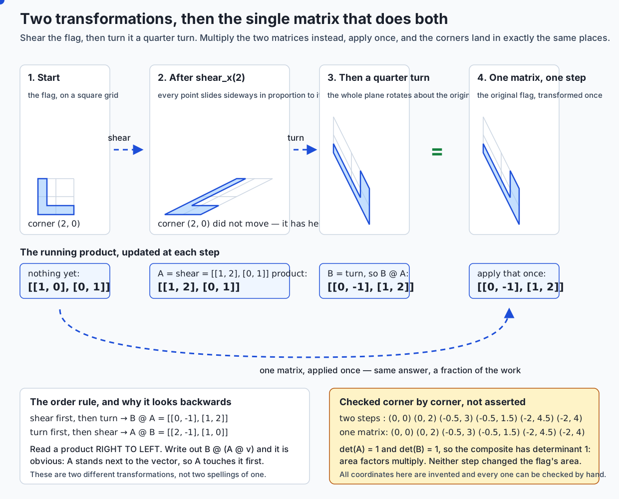
The order. compose(second, first) — and in matrix notation B @ A — means A happens first. The step that comes first is written on the right. This reads backwards until you write out what it means:
B @ (A @ v)A is the one standing next to the vector, so A is the one that touches it first. That is not a convention to memorise; it is what the notation says.
And it is not a spelling difference. The other order is a genuinely different transformation:
  compose(B, A)  shear then turn  = [(0.0, -1.0), (1.0, 2.0)]
  compose(A, B)  turn then shear  = [(2.0, -1.0), (1.0, 0.0)]
  the two products differ: True
  and they send (1.0, 1.0) to different places:
    shear then turn -> (-1.0, 3.0)
    turn then shear -> (1.0, 1.0)
Socks and shoes. Day 101 built the multiplication; today is the geometric reason it cannot commute.
The determinant, measured rather than defined
Most people meet the determinant as ad - bc, a formula with no visible reason. Meet it the other way round instead.
Take the unit square — corners (0, 0), (1, 0), (1, 1), (0, 1), listed anticlockwise. Its area is 1. Send it through a transformation and measure the area of what comes out. Here is that done, with the areas measured by the shoelace formula and the determinants computed separately:
  transformation      measured area   determinant   by hand
  scaling(2, 3)                 6.0           6.0       6.0
  shear_x(2)                    1.0           1.0       1.0
  reflection in x              -1.0          -1.0      -1.0
  collapse                      0.0           0.0       0.0
The measured area and the determinant are the same number every time, sign included. The determinant is not a formula that happens to be useful. It is the area factor.
Three readings, in increasing order of how much they matter:
Size. A determinant of 6 means every region comes out six times bigger. Not just the unit square — every region, because the sheet stretched uniformly. A determinant of 1 means area was preserved exactly, which is why a shear has determinant 1: sliding the cards of a deck sideways does not change how much deck there is.
Sign. A negative determinant means the plane was turned over. Watch what happens to the corners:
  before: [(0.0, 0.0), (1.0, 0.0), (1.0, 1.0), (0.0, 1.0)]
  after : [(0.0, 0.0), (1.0, 0.0), (1.0, -1.0), (0.0, -1.0)]
  signed area went from 1.0 to -1.0
The size did not change — the square is still area 1. What changed is that the corners now run clockwise. The fabric was lifted off the table and put back the other way up. No amount of rotating undoes that, the same way no amount of turning a left glove makes it a right one.
Zero. This is the one with consequences. Take [[1, 2], [2, 4]] and look at its columns: (1, 2) and (2, 4). The second is exactly twice the first. Both basis vectors land on the same line through the origin, so everything else does too — there is nowhere else left to land:
    (1.0, 0.0)   -> (1.0, 2.0)     on the line y = 2x: True
    (0.0, 1.0)   -> (2.0, 4.0)     on the line y = 2x: True
    (3.0, -1.0)  -> (1.0, 2.0)     on the line y = 2x: True
    (7.0, 7.0)   -> (21.0, 42.0)   on the line y = 2x: True
  the unit square becomes [(0.0, 0.0), (1.0, 2.0), (3.0, 6.0), (2.0, 4.0)]
  its area is 0.0
The whole plane has been flattened onto a line. And here is the cost:
  Two different starting points now share a landing place:
    (2, 0) -> (2.0, 4.0)
    (0, 1) -> (2.0, 4.0)
Two different inputs, one output. No rule can send that output back to both of them. The information is not hidden, compressed or encoded — it is gone. That is precisely what “no inverse” means, and it is why the geometric reading is worth having: “determinant zero” and “not invertible” and “the plane got flattened” are one fact wearing three hats.
| Determinant | Geometry | Invertible? | Rank (2×2) |
|---|---|---|---|
| Greater than 0 | Area scaled by that factor, orientation kept | yes | 2 |
| Exactly 1 | Area unchanged, orientation kept (rotations, shears) | yes | 2 |
| Less than 0 | Area scaled by the size, orientation flipped | yes | 2 |
| Exactly 0 | Plane flattened onto a line, or onto the origin | no | 1, or 0 |
An honest disagreement between two determinants
Building the lab turned up something worth reporting rather than smoothing over.
  P = [[3.0, -1.0], [1.0, 2.0]]
  by hand:            3 * 2 - (-1) * 1 = 7.0
  from-scratch:       7.0
  numpy.linalg.det:   7.000000000000001
  they differ by      8.881784197001252e-16
Neither is wrong. The from-scratch version computes a*d - b*c directly, which for four whole numbers is exact. numpy.linalg.det factorises the matrix first — the same general routine it uses on a 500×500 matrix, where the direct formula is not an option — and that factorisation rounds.
NumPy trades a last-bit error on a tiny input for a method that stays usable on a large one. That is a good trade, and knowing about it is what stops you writing if numpy.linalg.det(M) == 0 and being quietly wrong. Compare determinants with a tolerance, or better, ask numpy.linalg.matrix_rank.
This was observed on one machine, on one day, with numpy 2.5.2. No claim is made about other versions or other processors, because none were run.
The inverse, and when there is nothing to return
The inverse is the transformation that undoes this one — the matrix which, composed with the original, leaves everything exactly where it started.
For a 2×2 matrix it is 1 / determinant times [[d, -b], [-c, a]], and the important part of that formula is the division. It exists precisely when the determinant is not zero, which is the same sentence as “precisely when no area was destroyed”.
Most of the time you can write the inverse down without the formula, by asking what would undo the thing:
  shear_x(2)          [[1.0, 2.0], [0.0, 1.0]]
  its inverse         [[1.0, -2.0], [-0.0, 1.0]]
  which is shear_x(-2) -- push the deck of cards back the other way.
  inverse @ original = [[1.0, 0.0], [0.0, 1.0]]   the identity
  (1.0, 1.0) -> (3.0, 1.0) -> (1.0, 1.0)
That -0.0 is real and it is left in rather than tidied away. The formula divides -c by the determinant, and c here is 0.0, so the result is negative zero — a value binary floating point genuinely has and Python genuinely prints. It compares equal to 0.0, so nothing downstream notices, but you will meet it in printed output one day and it is better to have met it here.
The inverse of scaling(2, 3) is scaling by 1/2 and 1/3. The inverse of a rotation by θ is a rotation by -θ. The inverse of a reflection is the same reflection — do it twice and you are back, which the lab asserts.
And when there is nothing to return, both implementations say so:
  from-scratch inverse raises SingularMatrix: Singular matrix: the determinant is 0, so this transformation collapses the plane and cannot be undone
  numpy.linalg.inv raises LinAlgError: Singular matrix
A detail worth knowing, because it decides how you write the except clause: numpy.linalg.LinAlgError is a subclass of ValueError. The lab’s own SingularMatrix is defined as a ValueError subclass to match, so except ValueError catches either one and code written against one behaves the same against the other.
Rank, in plain language
Rank is how many dimensions survive.
Feed the whole plane in and look at what comes out. If the output still fills the plane, the rank is 2. If it is squashed onto a line, the rank is 1. If everything lands on the origin, the rank is 0.
For a 2×2 matrix you can read it off the columns without computing anything. If the two columns point in genuinely different directions, between them they reach everywhere and the rank is 2. If one column is a multiple of the other — as in (1, 2) and (2, 4) — everything lands on one line and the rank is 1. If both columns are zero, everything lands on the origin.
  identity                   rank 2   numpy.linalg.matrix_rank: 2
  scaling(2, 3)              rank 2   numpy.linalg.matrix_rank: 2
  shear_x(2)                 rank 2   numpy.linalg.matrix_rank: 2
  collapse                   rank 1   numpy.linalg.matrix_rank: 1
  everything to the origin   rank 0   numpy.linalg.matrix_rank: 0
For a square matrix, “full rank”, “non-zero determinant” and “invertible” are three names for one situation. Rank is the more useful word once matrices stop being square, because a non-square matrix has no determinant but still has a perfectly good answer to “how many dimensions survive”.
Why straight lines are a ceiling
Now the part this lesson exists for.
Fact one: the origin cannot move. M @ (0, 0) is zero lots of column 0 plus zero lots of column 1. There is no matrix anywhere that moves the origin. The lab checks this against seven different matrices, including a random twenty-layer product, and it holds every time.
Fact two: straight lines stay straight, and evenly spaced points stay evenly spaced. Take two points, take their midpoint, transform all three. The midpoint of the images is the image of the midpoint:
  p = (1.0, 3.0)   q = (4.0, -2.0)   midpoint of p and q = (2.5, 0.5)
  M @ midpoint            = (2.564582562299, 2.058012701892)
  midpoint of M@p and M@q = (2.564582562299, 2.058012701892)
  the same within 1e-12: True
Not just the midpoint. Eleven points spaced evenly along the line from p to q come out evenly spaced along a line, with a worst disagreement of 8.881784197001252e-16 — a rounding error, comfortably inside the stated tolerance and nowhere near a bend. A transformation that cannot bend a line cannot draw a curve — not “finds it hard”, cannot.
Fact three: a stack collapses. Which is where this lesson opened. Twenty matrices, applied one at a time versus multiplied first, agreeing to a relative 6.3e-16. Depth bought nothing, because M20 @ ... @ M2 @ M1 is a matrix, and it has been a matrix the whole time.
Put the three together and the exclusive-or arrangement from the opening is not merely hard for a stack of linear layers, it is out of reach. Class A on one diagonal and class B on the other cannot be split by a straight line; a stack of linear layers followed by a threshold can only ever cut with a straight line; and one of the four points is the origin, which cannot be moved at any weight setting whatsoever.
Now put something non-linear between the layers. ReLU — replace every negative number with zero — is the usual choice, and it is about as simple as a function can be while not being linear:
  M @ (1, -1)            = (0.066987, -1.116025)
  ReLU of that           = (0.066987, 0.0)
  relu(M @ (u + v))      = (2.098076, 2.366025)
  relu(M@u) + relu(M@v)  = (2.098076, 3.482051)
Those last two are not equal, so the composite fails additivity, so it is not linear, so it is not a matrix, so no algebra slides the layers together past it. The collapse stops working. Depth starts to buy something.
That is the honest answer to “why do we need activation functions”, and notice that it is not a claim about expressive power that you have to take on trust. It is a claim about a collapse you can watch happening, and about a specific arithmetic identity that the non-linearity breaks.
An everyday analogy
Back to the pinned sheet, and let us push it until it breaks, because an analogy you have not tested is a liability.
The sheet is graph paper printed on stretchy fabric, with a pin through the origin. Pulling the sheet is applying a matrix.
- The pin is the origin. It never moves, in any transformation, ever. When you need the whole sheet shifted sideways, you cannot do it by pulling — you have to unpin it and move the pin, and that is the
+ binX @ W + b. Not linear, kept separate, and now you know why it is kept separate rather than folded in. - The two arrows drawn next to the pin are e1 and e2. Where they end up is the matrix. Everything else on the sheet is dragged along by them.
- Pulling harder horizontally than vertically is scaling. Sliding the top edge sideways while the bottom stays put is a shear. Spinning the whole sheet around the pin is a rotation. Lifting the sheet and putting it back face down is a reflection.
- The printed unit square becomes a parallelogram. How many times bigger it got is the determinant. If you put the sheet back face down, the printed labels read backwards and the determinant is negative.
- Pull the sheet, then pull it again a different way. Somebody watching only the start and the end sees one pull. That is composition, and it is why twenty pulls are one pull.
- Squash the sheet flat against a ruler so the whole thing lies along one line. That is determinant zero. Two printed points that were far apart are now on top of each other, and no pulling gets them apart again, because the sheet does not remember which one was which. That is rank 1, and it is why there is no inverse.
Where the analogy holds up. It gets the origin right, the straightness right, the area right, the flip right, the collapse right, and composition right. It also correctly predicts that a stack of pulls is one pull, which is the whole lesson.
Where it breaks, and you should know. The fabric is finite and the plane is not — a real transformation acts on every point out to infinity, so “the sheet ran out” is never a thing that happens. Real fabric also resists, and stretches non-uniformly at the edges; a linear transformation is perfectly uniform everywhere, and if your mental picture ever has the grid bunching up in one corner, that picture has stopped being linear. And a physical sheet cannot pass through itself, so it cannot model a determinant-zero collapse without tearing — the mathematics is perfectly happy to squash infinitely many points onto one line, and the fabric is not.
Crumpling is the important forbidden move. The moment you crumple, curve, or fold the sheet, you have left linear algebra — and that is exactly what an activation function does. ReLU is the crumple.
Examples in practice
A neural network layer. X @ W + b, then an activation. Everything in this lesson applies to the X @ W part: W is a transformation, its columns are landing places, its rank tells you how many dimensions of the input survive into the output, and its determinant (when it is square) tells you what it does to volume. The + b is bolted on because a matrix cannot move the origin. The activation is bolted on because otherwise the layers collapse. Both additions exist for reasons this lesson has now measured.
Dimensionality reduction. Projecting a 768-dimensional embedding down to 2 for a scatter plot is a linear transformation with a rank of at most 2. That is a determinant-zero situation in the strongest sense — you are deliberately destroying 766 dimensions of information because you want a picture. Understanding that the destruction is real and permanent is the difference between reading such a plot carefully and over-reading it. Points that look close in the picture may have been nowhere near each other before the collapse.
Whitening and normalisation. Rotating a dataset onto its own principal axes and rescaling each axis is scaling composed with rotation, which composes into a single matrix, which is applied once. Days ahead cover the finding of those axes; today gives you the vocabulary for what is being done once they are found.
Graphics, and Day 105. Rotating, scaling and shearing an image is exactly this lesson applied to pixel coordinates, and it is the Week 15 project. There is one wrinkle worth flagging now so it does not surprise you: image libraries generally specify the transform as the map from output pixel back to input pixel — the inverse of the visual effect — because that is the direction you need in order to fill every output pixel exactly once. I ran a small check with Pillow 12.3.0 here to confirm that direction: with the coefficient tuple (1, 0, 1, 0, 1, 0), a bright pixel at input x = 3 appeared in the output at x = 2, so the content moved left when the parameter said +1. That is the inverse-mapping convention, confirmed rather than assumed. The remaining details — including a half-pixel sampling offset that makes a shear coefficient appear to act even on row 0 — are Day 105’s business, and this lesson will not assert them from memory.
Where you have already met it without noticing. The transform property in CSS and the transform attribute in SVG both take a matrix(...) function whose arguments are, in order, the two columns of a 2×2 matrix followed by a translation. Six numbers: four for the linear part, two for the shift that the linear part cannot do. Homogeneous coordinates in the wild.
Implications: security, privacy, performance, scalability, and cost
Performance. Composition is the whole story. Twenty transformations applied to a million points is twenty million operations; multiply the twenty matrices first and it is one million plus twenty tiny products. Both give identical answers. This generalises directly: whenever a fixed pipeline of linear steps is applied to a lot of data, fold the pipeline first.
The second performance point is the flip side of the opening. Because consecutive linear layers collapse, a “deep” stack of them is wasted computation — you paid for twenty matrix multiplications and received one matrix’s worth of capability. That is not a subtle inefficiency; it is a total one.
Cost. Same argument, in money. A folded pipeline costs a twentieth of an unfolded one at inference time, and the saving compounds over every request for the lifetime of the service.
Scalability. A transformation is a fixed-size object no matter how much data flows through it. Four numbers in two dimensions, n² in n dimensions, and that is all you ever store or send. This is why a model’s weights are small compared with its training data, and why shipping a model is shipping a modest file rather than a dataset.
Privacy, and the claim to be suspicious of. “We reduced the dimensions, so the original data cannot be recovered” is a claim about rank, and it is checkable in one line. If the transformation has full rank, the reduction was lossless and what looked like anonymisation was a reversible relabelling — anyone with the matrix can invert it and get the original back. If the rank is genuinely lower than the input dimension, information really was destroyed, and the determinant-zero argument above says it is destroyed permanently.
The check is numpy.linalg.matrix_rank, and it is worth running before anyone builds a policy on top of an assumption. Note also that low rank is not by itself a privacy guarantee: it says some information is gone, not that the identifying information is gone.
Security. A determinant-zero step is a one-way door, and that is sometimes precisely the property you want — if two different inputs must be indistinguishable afterwards, you need a step from which they cannot be told apart. It is also, more often, the property that bites: a pipeline that collapses somewhere in the middle cannot be inverted after that point, and “we can always reconstruct the original from the embedding” is a claim to verify rather than assume.
Numerical cost, which is the one that surprises people. A matrix can be invertible in exact arithmetic and effectively uninvertible in floating point. If the determinant is not zero but is very close to it, the inverse involves dividing by a tiny number, and every rounding error in the input gets multiplied by a huge factor on the way out. The answer is not wrong in an obvious way — it is wrong in a plausible-looking way. This is why the practical question is rarely “is the determinant zero” and usually “how close to a collapse is this”, and why production code reaches for numpy.linalg.solve rather than computing an inverse and multiplying by it.
Alternatives: free, open source, and commercial
The honesty statement first, because it decides how to read everything below. Only NumPy 2.5.2 and Pillow 12.3.0 were actually run for this lesson. Every output block above came from a real run on the authoring machine. The other tools in this section are described from their published documentation and their behaviour is not reproduced here, because they are not installed. Where a claim needed checking, it was checked; where it could not be, it is not asserted.
NumPy — free, open source, BSD 3-Clause. Ran here.
The default, and the right default for learning. Everything today’s lab checks against came from it.
When to choose it: any numerical work in Python that fits in memory on one machine, which is most work.
How to use it, in four lines:
import numpy as np
M = np.array([[3.0, -1.0], [1.0, 2.0]])
M @ np.array([2.0, 1.0])            # apply: array([5., 4.])
np.linalg.det(M), np.linalg.matrix_rank(M), np.linalg.inv(M)
The concrete example, from this lesson’s real output: np.linalg.inv on [[1, 2], [2, 4]] raises LinAlgError: Singular matrix, and np.linalg.det on [[3, -1], [1, 2]] returns 7.000000000000001 rather than 7.0. Both were run; both are quoted exactly.
Free vs paid: entirely free. No tier, no account, no key.
SciPy scipy.linalg — free, open source. Not installed here; no output reproduced.
When to choose it: when NumPy’s linear algebra is not enough — decompositions NumPy does not carry, matrix functions such as the matrix exponential, and specialised solvers for structured matrices. Its documentation describes scipy.linalg as a superset of numpy.linalg built on the same underlying LAPACK routines.
How you would use it: the same shapes and the same array objects; you import from scipy.linalg instead of numpy.linalg.
Free vs paid: entirely free.
PyTorch — free, open source. Not installed here; no output reproduced.
When to choose it: when the transformation is something you want to learn rather than write down. That is the whole difference. In this lesson the four numbers of a matrix were chosen by you, derived from geometry; in a network they are found by gradient descent, and PyTorch exists to compute those gradients and to run the arithmetic on a GPU.
How you would use it: the @ operator works on tensors as it does on arrays, and the linear algebra routines live under torch.linalg with names deliberately mirroring NumPy’s. A torch.nn.Linear layer is X @ W.T + b — the linear transformation of this lesson, plus the bias that cannot be folded into it.
Free vs paid: the library is free. The GPU it likes to run on is not, whether you buy one or rent one, and that is where the money in modern machine learning actually goes.
Graphics and image tools — mostly free. Only Pillow was run here.
CSS and SVG both express 2D transforms as matrix(a, b, c, d, e, f): the first four numbers are the two columns of the linear part and the last two are the translation, which is exactly the homogeneous-coordinate arrangement described earlier. Image libraries such as Pillow, and the transform tools inside any image editor, are doing the same arithmetic on pixel coordinates.
The one thing verified here: Pillow’s affine coefficients express the map from output pixel back to input pixel — the inverse of the visual effect. Confirmed by running it, as described in the previous section. Everything else about these tools is left to Day 105, which applies all of this to a real image and can quote real output for it.
Free vs paid: Pillow, CSS and SVG are free. Commercial image editors are not, and none is required for anything in this course.
Doing it by hand, with math and nothing else — free, and the one you should start with.
When to choose it: exactly once, which is today. The entire from-scratch module in this lab imports nothing but math, and that is deliberate. If your rotation function were built from a NumPy helper, then checking it against NumPy would be checking NumPy against itself. Writing the arithmetic yourself and then having a mature library agree with you is worth more than either half alone.
When not to: every day after today. Your hand-written version is slower, unvectorised, two-dimensional and untested against decades of edge cases.
Comparison with related concepts
| Concept | What it is | How it differs from a linear transformation |
|---|---|---|
| Affine transformation | Linear, plus a shift: x ↦ M @ x + b | Does not fix the origin, so it fails both linearity conditions. Every network layer is one. Graphics systems make it look linear using homogeneous coordinates. |
| Non-linear function | Anything else — ReLU, sigmoid, squaring | Cannot be written as a matrix at all, at any size. This is what makes depth worth having. |
| Matrix multiplication (Day 101) | The arithmetic | Today is the meaning: multiplication is composition, and Binet defined it that way in 1812. |
| Dot product (Day 103) | Two vectors in, one number out | Not a transformation of the plane — the output is not a vector. It is one row of a matrix–vector product, in isolation. |
| Eigenvector (Day 106) | A direction the transformation does not turn | A property of a linear transformation. Today asks where everything goes; eigenvectors ask what stayed pointing the same way. |
| Change of basis | Describing the same vectors in different coordinates | Mechanically identical — a matrix — but the interpretation is inverted. Nothing moved; the description changed. |
| Permutation | Reordering entries | A special linear transformation whose matrix has one 1 per row and column. Determinant +1 or -1, always invertible, never changes size. |
| Projection | Flattening onto a subspace | A linear transformation with determinant 0 and reduced rank. The interesting sub-case of a collapse: deliberate, and irreversible on purpose. |
When to use it — and when not to
Reach for this framing when:
- A shape error or a surprising result makes you ask what a matrix in your pipeline actually does. “Where do the basis vectors land” answers it faster than reading the numbers.
- You have a fixed sequence of linear steps and a lot of data. Compose first.
- Somebody claims a transformation is irreversible, or that it is reversible. Both are one call to
matrix_rankaway from being settled. - You are deriving something geometric — a rotation, a reflection about an unusual line, a projection — and cannot remember the formula. Derive it from two landing places instead.
Do not reach for it when:
- The relationship you are modelling is genuinely curved. No matrix, and no stack of matrices, will fit it. This is a limitation to respect, not to work around with more layers.
- You need a shift. A matrix cannot move the origin. Add the bias, or move to homogeneous coordinates, and be clear about which you have done.
- You are tempted to compute an explicit inverse in production code. Prefer
numpy.linalg.solve; it is more accurate and usually faster, and it does not tempt you into reusing an inverse that a nearly-singular matrix made meaningless. - The dimensions are large and the matrix is mostly zeros. The geometric intuition still holds, but a dense 2×2 mental model does not tell you anything useful about the memory behaviour of a sparse 100,000-dimensional operator.
Where this goes next in AI work
Every layer in every network you will build is a linear transformation followed by a non-linear function. The linear part is what this lesson described completely — columns as landing places, composition as multiplication, determinant as area, rank as surviving dimensions. The non-linear part exists because of the ceiling this lesson measured.
That framing pays off almost immediately. A weight matrix with a rank much lower than its size is a layer that is quietly throwing away dimensions, whatever its shape says. A pipeline of linear steps with no activation between them is a bug that trains without complaining. And an embedding projected to two dimensions for a plot is a determinant-zero collapse that you chose on purpose, with all the loss of information that implies.
Day 103 takes the dot product — one row of what you did today, in isolation — and turns it into a measure of similarity. Day 105 applies today’s four matrices to a real image, where a shear and a rotation stop being abstractions and become something you can look at. And Day 106 asks the question this lesson deliberately left alone: when you pull the sheet, are there any directions that do not turn at all?
Knowledge check
Eight questions on today’s material are in quiz.yml and appear on the lesson page. Two of them are worth attempting before you read another word: one asks you to read a transformation off the columns of a matrix, and one asks what a zero determinant actually means. If those two come easily, the day has landed.
Hands-on exercise
The lab is “Where Do the Basis Vectors Land?”, and it builds the whole of this lesson from arithmetic.
You write ten functions in starter/transforms.py using nothing but math: from_landings, columns_of, apply, scaling, reflection_in_x_axis, shear_x, rotation, compose, determinant and inverse. Then you make thirty-one predictions in starter/answers.py, each of which you can work out on paper in under a minute — where a matrix off a described picture sends (2, 1), whether f(v) = M @ v + b is linear and by how much it fails, which product means “shear first”, what the signed area of the unit square is after a reflection, the rank of a collapse, and the exact exception class numpy.linalg.inv raises on it.
A test suite scores you as you go. Unattempted work is skipped, not failed, so your score only ever counts work you actually did.
cd labs/sections/math-statistics-and-data/day-102-linear-transformations
python3 -m venv .venv
.venv/bin/pip install -r requirements/requirements.txt
.venv/bin/pytest starter -q
Expected output
An untouched checkout scores like this:
.sssssssssssssssssssssssssssssssssssssssssssssssssssss                   [100%]
1 passed, 53 skipped in 0.06s
When you have finished it says 54 passed.
Once you have tried, read the reference. Six scripts, each printing its working and asserting every claim it makes. Script 05 measures the determinant:
  transformation      measured area   determinant   by hand
  scaling(2, 3)                 6.0           6.0       6.0
  shear_x(2)                    1.0           1.0       1.0
  reflection in x              -1.0          -1.0      -1.0
  collapse                      0.0           0.0       0.0
and shows what a collapse costs:
  Two different starting points now share a landing place:
    (2, 0) -> (2.0, 4.0)
    (0, 1) -> (2.0, 4.0)
and what both libraries do when asked to undo it:
  from-scratch inverse raises SingularMatrix: Singular matrix: the determinant is 0, so this transformation collapses the plane and cannot be undone
  numpy.linalg.inv raises LinAlgError: Singular matrix
The full harness ends with:
64 checks, 0 failure(s).and exits 0.
Validate your work
bash tests/run_tests.sh; echo "exit=$?"prints64 checks, 0 failure(s).andexit=0..venv/bin/pytest examples -q -p no:cacheproviderprints80 passed..venv/bin/pytest starter -q -p no:cacheproviderprints54 passedwhen you are done.- Each of the six reference scripts ends with
every assertion held. find . -type d -name '__pycache__' -o -type d -name '.pytest_cache'prints nothing after a full run.
Section 6 of the harness is worth watching: it re-runs itself with one expectation deliberately swapped for the naive belief that cos(π / 2) is exactly 0.0, and asserts that the re-run exits non-zero and reports exactly one failure. A green suite proves nothing until you have seen it go red.
Troubleshooting
ModuleNotFoundError: No module named 'transforms'— you ran a reference script from the lab directory rather than from insideexamples/. The scripts import their neighbours.cd examplesfirst; run the pytest commands from the lab directory.- A test failed with
NotImplementedErrorinstead of skipping — this happened while building the lab. Python evaluates arguments before the call, sowritten(compose, rotation(...), shear_x(...))callsrotationfirst, and an unwritten function escapes before the skip mechanism runs. The suite now wraps whole bodies in a callable. If you add tests, do the same. - The starter tests pass without me writing anything — you ran a bare
pytestand an import guard is missing. Both directories contain modules calledtransformsandshapes; eachconftest.pystops one suite importing the other’s. Restore it withgit checkout -- starter/conftest.py. cos(pi / 2)prints6.123233995736766e-17— correct, expected, and asserted by one of the reference tests. Use the stated tolerance;== 0.0fails on a right answer.numpy.linalg.detgives7.000000000000001— also correct and also asserted. See the section above on the two determinants.numpy.linalg.LinAlgError: Singular matrix— the intended result of the collapse exercise, not a fault.
troubleshooting.md in the lab covers each of these at length, plus the wrong-direction rotation and the Windows path differences.
Common mistakes
| Mistake | What it looks like | The fix |
|---|---|---|
| Reading a row as a landing place | Confidently writing (3, -1) as where e1 went | The matrix is written across and means down. Column 0 is (3, 1). |
| Getting the composition order backwards | A @ B when you meant “A first” | The first step goes on the right. Write out B @ (A @ v) and it is obvious. |
| Signs swapped in the rotation matrix | rotation(π/2) sends (1, 0) to (0, -1) — clockwise | The minus belongs on the -sin θ in the top right, which is the first coordinate of where (0, 1) lands. |
Comparing floats with == | A correct quarter turn “fails” a test | State a tolerance and say why. 1e-12 here. |
if numpy.linalg.det(M) == 0 | A singular matrix passes as invertible, or a fine one is rejected | Use a tolerance, or numpy.linalg.matrix_rank. |
| Assuming a shear changes area | Surprise that det is 1 | Draw the sheared square. Same base, same height, same area. |
| Believing more linear layers add capacity | A model that will not train and has no error message | Twenty linear layers are one linear layer. Put a non-linearity between them. |
Practice assignment
Work these in a scratch file next to the lab. Every one is checkable in a few lines.
-
Reflection in the line
y = x. Derive the matrix by asking where(1, 0)and(0, 1)land under that mirror. Predict the determinant before computing it, and say why the sign is what it is. -
The projection onto the x axis. Build the matrix that sends every point
(x, y)to(x, 0). State its determinant and its rank before running anything, then name two distinct points that became indistinguishable. Explain in one sentence why no inverse can exist. -
Order, measured. Take
scaling(2, 1)androtation(π / 4). Compute both products. Apply each to(1, 0)and to(0, 1)and describe, in words, how the two resulting shapes differ. Then find a pair of transformations that do commute, and say what they have in common. -
The determinant of a product. Verify on three examples of your own that
det(B @ A) = det(A) · det(B). Then answer without computing: if one step in a ten-step pipeline has determinant 0, what is the determinant of the whole pipeline, and what does that tell you about recovering the input? -
Break linearity in a second way. The lesson’s non-linear example was “add a constant”. Find a function that does fix the origin and is still not linear — squaring one coordinate will do — and demonstrate the failure with the same two tests. This matters because it shows that fixing the origin is necessary for linearity and not sufficient.
-
The tolerance question. Find a 2×2 matrix of small decimals whose true determinant is 0 but for which
numpy.linalg.detreturns something other than0.0. Then decide what tolerance you would use in production code to call a matrix singular, and write down one thing that could go wrong with a tolerance that is too tight and one with a tolerance that is too loose.
Extension challenge
Build a shape classifier that cannot work, then make it work.
Write the four exclusive-or points from the opening of this lesson into an array with their labels. Then:
-
Write a function that takes a list of 2×2 matrices and a point, applies them in sequence, and returns the sign of the first coordinate as a predicted class. This is a stack of linear layers with a threshold at the end.
-
Search for weights that classify all four points correctly. Do it however you like — random search over a few hundred thousand candidates is fine and takes seconds. Record the best accuracy you achieve.
-
Now prove that your failure was not bad luck. Multiply your matrices together into one, and show that the stack of any depth is a single 2×2 matrix. Then show that
(0, 0)maps to(0, 0)under it, whatever the weights, and reason about what that alone implies for classifying a point at the origin. -
Insert a single ReLU between two of the layers and repeat the search. Report what changed, and confirm by the additivity test that the composite is no longer linear.
-
Finally, write a short paragraph — for yourself, in the file — explaining to a version of you from last week why “add more layers” was never going to work. If you can write that paragraph without using the phrase “non-linear”, you understand it.
Everything you need is in today’s lab: compose, apply, determinant and is_linear. Nothing else is required, and no library beyond NumPy.
Quiz
Q1. A picture shows the arrow (1, 0) redrawn ending at (3, 1), and the arrow (0, 1) redrawn ending at (-1, 2). What is the matrix?
- [[3, 1], [-1, 2]] — the two landing places written as rows
- [[3, -1], [1, 2]] — the two landing places written as columns
- [[1, 0], [0, 1]] — the picture does not determine a matrix on its own
- [[3, -1], [1, 2]] transposed, because NumPy stores arrays row-major
Show answer
Answer: B. [[3, -1], [1, 2]] — the two landing places written as columns
The columns are the landing places. Column 0 is where (1, 0) went, read downwards, so the left column is 3 above 1. Column 1 is where (0, 1) went, so the right column is -1 above 2. Written as rows that is [[3, -1], [1, 2]]. Option 0 is the single most common mistake in the whole topic: the matrix is written across and it means down, so row 0 here is (3, -1) and nothing lands there. Option 2 is wrong because two landing places settle everything — every vector is a combination of the two basis vectors, and a linear transformation preserves combinations, so knowing where those two go fixes where all the others go. Option 3 confuses how NumPy lays bytes out in memory with what a matrix means; storage order is a Day 100 topic and has nothing to do with this.
Q2. A transformation has determinant 0. What does that tell you?
- It shrinks every shape to a very small area, but nothing is lost
- It leaves area unchanged, like a rotation or a shear
- It flips the plane over, so shapes come out mirrored
- It flattens the plane onto a line or a point, two different inputs can share an output, and it cannot be undone
Show answer
Answer: D. It flattens the plane onto a line or a point, two different inputs can share an output, and it cannot be undone
The determinant is the factor by which area is multiplied, so a determinant of 0 means the unit square came out with area 0 — the plane was flattened. On [[1, 2], [2, 4]] both columns lie along the line y = 2x, so everything lands on that one line, and the lab shows (2, 0) and (0, 1) both landing on (2.0, 4.0). Two different starting points now share a landing place, and no rule can send that place back to both of them. The information is not compressed or hidden, it is gone, which is exactly what "no inverse" means: numpy.linalg.inv raises LinAlgError: Singular matrix. The first option is the reassuring misreading — 0 is not "very small", it is a collapse, and the difference is the difference between lossy and total. The second describes determinant 1. The third describes a NEGATIVE determinant, which flips orientation while keeping the size.
Q3. Which of these functions is linear?
- f(v) = M @ v + b, with b = (1, 1) — a network layer
- f(x, y) = (x squared, y)
- f(v) = M @ v
- f(x, y) = (x + 1, y + 1)
Show answer
Answer: C. f(v) = M @ v
Linear means exactly two things: f(u + v) = f(u) + f(v), and f(cu) = c f(u). Only multiplication by a matrix satisfies both. Options 0 and 3 both move the origin — f((0, 0)) is (1, 1), not (0, 0) — and no linear transformation can move the origin, because M @ (0, 0) is zero lots of each column. That is the one-second test, and it disposes of both without touching a pair of vectors. The gap in option 0 is measurable and instructive: f(u) + f(v) minus f(u + v) comes out as exactly b, because the offset is added once on one side and twice on the other. Option 1 is the interesting case, and it is why the origin test is necessary but not sufficient: squaring a coordinate DOES fix the origin and is still not linear, because doubling the input quadruples the first output instead of doubling it. Option 0 is called affine — linear plus a shift — and it is the shape of every layer in every network you will build.
Q4. You want to shear a shape first and then rotate it. Which single matrix does both?
- A @ B, where A is the shear and B is the rotation
- B @ A, where A is the shear and B is the rotation
- Either — matrix multiplication is commutative for rotations
- Neither; two transformations cannot be written as one matrix
Show answer
Answer: B. B @ A, where A is the shear and B is the rotation
The step that happens FIRST is written on the RIGHT. Write out what applying A and then B to a vector means — B @ (A @ v) — and it is obvious: A is the one standing next to the vector, so A touches it first. The identity B(Ax) = (BA)x is what lets you collapse the two into one. This is not a convention to memorise, it is what the notation says. Option 0 is a genuinely different transformation, not a different spelling: with A = shear_x(2) and B = a quarter turn, B @ A is [[0, -1], [1, 2]] while A @ B is [[2, -1], [1, 0]], and they send (1, 1) to (-1, 3) and (1, 1) respectively. Option 2 is false — matrix multiplication is non-commutative in general, and Wikipedia says so in as many words. Option 3 is exactly backwards: composing into one matrix is the reason matrix multiplication was defined at all, by Binet in 1812.
Q5. A transformation has determinant -1. What happened to the unit square?
- It kept its area of 1, but the plane was turned over, so its corners now run the other way round
- Its area became -1, which is impossible, so the matrix is invalid
- It shrank to nothing
- It was rotated by 180 degrees
Show answer
Answer: A. It kept its area of 1, but the plane was turned over, so its corners now run the other way round
The SIZE of the determinant is the area factor and the SIGN is the orientation. A determinant of -1 means the area is still 1 and the plane was flipped. Measured in the lab: the unit square listed anticlockwise has signed area +1, and after reflection in the x axis its corners are (0, 0), (1, 0), (1, -1), (0, -1) with signed area -1. Same size, opposite winding. No rotation undoes it, the same way no amount of turning a left glove makes it a right one — and that is why the last option is wrong: a 180 degree rotation has determinant +1, not -1, and the lab checks that every rotation, at every angle it tries, has a positive determinant. The second option misreads a signed quantity as a physical area; the sign is carrying extra information, not describing an impossible region. The third describes determinant 0, which is a different and much more serious event.
Q6. Why does a neural network layer compute X @ W + b instead of folding the bias into the weight matrix?
- For historical reasons; modern frameworks could fold it in but keep the old form for compatibility
- Because a matrix cannot move the origin, and b exists precisely to move it
- Because folding it in would make the matrix too large to fit in GPU memory
- Because the bias is trained separately from the weights, on a different objective
Show answer
Answer: B. Because a matrix cannot move the origin, and b exists precisely to move it
M @ (0, 0) is zero lots of column 0 plus zero lots of column 1, which is (0, 0) whatever the four numbers are. There is no matrix anywhere that moves the origin. So a shift cannot be expressed as a matrix multiplication in the same space, and it has to arrive separately, afterwards. Linear plus a shift has its own name — affine — and the separateness is structural, not stylistic. Option 0 is wrong because it could not be folded in: this is a mathematical impossibility, not a convention. Option 2 is wrong on size — the homogeneous-coordinate trick, which graphics systems do use to make translation look like a multiplication, grows an n by n matrix to (n+1) by (n+1), which is a rounding error in memory terms. Option 3 is wrong: weights and biases are trained together on the same objective by the same gradient step.
Q7. You write assert rotation(math.pi / 2) == [[0.0, -1.0], [1.0, 0.0]] and it fails. Why?
- The rotation matrix has the minus sign in the other position
- math.pi is only accurate to about six decimal places
- Lists cannot be compared with == in Python
- math.cos(math.pi / 2) is 6.123233995736766e-17, not 0.0, so the comparison must use a tolerance
Show answer
Answer: D. math.cos(math.pi / 2) is 6.123233995736766e-17, not 0.0, so the comparison must use a tolerance
Pi cannot be stored exactly in binary floating point, so the value handed to cos is not quite pi over 2, and its cosine is not quite zero — it is about 6.1e-17. The same thing happens to sin of 30 degrees, which comes out as 0.49999999999999994. Neither is a bug and neither is fixable; it is what binary floating point is. So every float comparison in this lab states a tolerance of 1e-12 and none use ==, and one of the reference tests asserts the inexactness itself so that the claim cannot quietly stop being true. The first option describes a real and common bug — signs swapped gives a clockwise rotation — but it is not what is happening here, and you can tell the two apart in one line by checking whether (1, 0) went up to (0, 1) or down to (0, -1). The second badly understates the accuracy: a Python float carries roughly fifteen to sixteen significant decimal digits, which is exactly why the error turns up at the seventeenth. The third is simply false; lists compare elementwise with == quite happily, which is how this assertion managed to run and fail rather than raise.
Q8. Twenty matrix layers are applied one after another, with nothing between them. What can the stack do that one layer cannot?
- Nothing — the twenty multiply together into a single matrix of the same size
- It can fit curved decision boundaries, which is why depth helps
- It can move the origin, once there are enough layers
- It can achieve any transformation, including non-linear ones, given enough width
Show answer
Answer: A. Nothing — the twenty multiply together into a single matrix of the same size
Composition of linear transformations is a linear transformation, so M20 @ ... @ M2 @ M1 is one matrix and always was. The lab measures it: twenty pseudo-random 2 by 2 matrices applied one at a time give (-3.5017165700891133, -4.824470758326175), and the single combined matrix gives (-3.501716570089111, -4.824470758326172), a relative difference of 6.3e-16 — the same answer to the limits of arithmetic. Depth bought nothing, and options 1, 2 and 4 are all versions of the same wrong hope. The stack still fixes the origin, still sends straight lines to straight lines, and still cannot separate the four exclusive-or points from the start of the lesson. This is the whole reason a non-linear activation sits between the layers: it breaks the additivity identity that lets the matrices slide together, so the collapse stops working and depth starts to buy something.
Glossary
- Linear transformation
- A function taking a vector and returning a vector that satisfies exactly two conditions: it preserves addition, so f(u + v) equals f(u) + f(v), and it preserves scalar multiplication, so f(cu) equals c f(u). Nothing else is in the definition. Every geometric fact about them — that the origin never moves, that straight lines stay straight, that evenly spaced points stay evenly spaced — is a consequence of those two lines rather than an addition to them. In two dimensions every such function can be written as a 2 by 2 matrix, and every 2 by 2 matrix is one.
- Basis vector
- One of a small set of vectors from which every other vector in the space can be built by scaling and adding. In the plane two are enough, and knowing where a linear transformation sends them determines where it sends everything else — which is the single most useful fact in the subject.
- Standard basis
- The particular pair e1 = (1, 0) and e2 = (0, 1) in two dimensions: one step right and one step up. Every vector (x, y) is x lots of e1 plus y lots of e2, which is what makes their landing places sufficient to describe a whole transformation. Written as e1, e2 and so on up to en in n dimensions.
- Transformation matrix
- The matrix whose columns are the landing places of the basis vectors: column 0 is where e1 goes, column 1 is where e2 goes. Formally A = the matrix whose columns are T(e1), T(e2) and so on. The most common error in the whole topic is reading a ROW as a landing place — the matrix is written across and it means down.
- Scaling
- Stretching or shrinking along the axes, with matrix [[sx, 0], [0, sy]]. Derived rather than remembered: one step right becomes sx steps right, so e1 lands at (sx, 0); one step up becomes sy steps up, so e2 lands at (0, sy). Its determinant is sx times sy, which is why scaling by 2 and 3 makes every area six times bigger.
- Reflection
- A mirroring of the plane in some line through the origin, with matrix [[1, 0], [0, -1]] for the x axis. Derived by noticing that a point ON the mirror line cannot move, so e1 stays put, while e2 goes from one step up to one step down. Its determinant is always -1: the size is preserved and the orientation is reversed, so a shape listed anticlockwise comes out listed clockwise.
- Shear
- A sideways slide in proportion to height, with matrix [[1, k], [0, 1]] for the horizontal case. The deck of cards pushed over: the bottom card does not move, every card above it slides further. e1 has height 0 so nothing pushes it; e2 has height 1 so it lands at (k, 1). Its determinant is exactly 1, because sliding the cards changes no areas — the sheared square has the same base and the same height as the original.
- Rotation matrix
- The matrix [[cos t, -sin t], [sin t, cos t]], which turns the whole plane anticlockwise by t radians about the origin. Derived from the unit circle in two steps: e1 walks around the rim to (cos t, sin t), which is the definition of those two functions, and e2 — already a quarter turn ahead — lands a quarter turn ahead of that, at (-sin t, cos t). Its determinant is cos squared plus sin squared, which is 1 by Pythagoras, so a rotation never changes area and never flips.
- Radian
- An angle measured as the distance walked around the rim of a circle of radius 1. The whole circumference is 2 pi, so a full turn is 2 pi radians, a half turn is pi and a quarter turn is pi over 2. Every trigonometric function in Python takes radians; math.radians converts from degrees.
- Composition
- Doing one transformation and then another. The single matrix that does both is the product of the two, with the FIRST step written on the RIGHT: applying A then B is B @ A, because A is the one standing next to the vector in B @ (A @ v). Matrix multiplication was defined by Binet in 1812 precisely to be this operation, which is why it does not commute — putting on socks then shoes is not the same as shoes then socks.
- Determinant
- The signed factor by which a transformation multiplies area, equal to a*d - b*c for a 2 by 2 matrix [[a, b], [c, d]]. Best met by measuring rather than by formula: send the unit square through and the signed area of what comes out IS the determinant. Its size is the area factor, its sign is the orientation, and a value of zero means the plane was flattened onto a line and nothing can undo it.
- Orientation
- Which way round a shape is wound — anticlockwise or clockwise. A positive determinant preserves it and a negative one reverses it, meaning the plane was turned over. No rotation undoes a reversal, in the same way no amount of turning a left glove makes it a right one. Measured by the sign of a polygon area computed with the shoelace formula.
- Singular matrix
- A square matrix whose determinant is zero, so it has no inverse. Geometrically it flattens the space: for a 2 by 2 matrix both columns lie along the same line, so every vector lands on that line and two different starting points can share a landing place. numpy.linalg.inv raises LinAlgError with the message "Singular matrix" rather than returning anything, and because LinAlgError is a subclass of ValueError, except ValueError catches it.
- Inverse
- The transformation that undoes another one, so that composing the two gives the identity. For 2 by 2 it is one over the determinant times [[d, -b], [-c, a]], and it exists precisely when the determinant is not zero — the same sentence as "precisely when no area was destroyed". Often writable by reasoning rather than formula: the inverse of shear_x(2) is shear_x(-2), of scaling by 2 and 3 is scaling by a half and a third, and of a reflection is the same reflection.
- Rank
- How many dimensions survive the transformation. Feed the whole plane in: if the output still fills the plane the rank is 2, if it is squashed onto a line the rank is 1, if everything lands on the origin the rank is 0. For a 2 by 2 matrix it reads off the columns — two columns pointing in genuinely different directions give rank 2, one column being a multiple of the other gives rank 1. numpy.linalg.matrix_rank computes it, and it is the more useful word than "determinant" once matrices stop being square.
- Identity matrix
- The matrix that leaves every vector exactly where it found it, [[1, 0], [0, 1]] in two dimensions. Under today reading it has a reason rather than a definition: it is what you write down when the basis vectors did not move, so nothing else moves either. Its determinant is 1 and its rank is full. numpy.eye(n) builds one.
- Affine transformation
- A linear transformation followed by a shift: x maps to M @ x + b. It is NOT linear, because it moves the origin and therefore fails both conditions — the additivity failure is exactly b and the scaling failure is exactly (s - 1) times b. Every neural network layer is affine, which is why the bias is written separately as X @ W + b: a matrix cannot move the origin, and b exists to move it.
- Homogeneous coordinates
- A trick that makes a shift look like a matrix multiplication by writing a 2D point (x, y) as the 3D vector (x, y, 1), whereupon translation becomes an ordinary 3 by 3 matrix product. It is why a 2D graphics transform is a 3 by 3 matrix and why CSS and SVG take six numbers for a 2D transform: four for the linear part and two for the shift. The shift did not become linear; it was moved to a bigger space where it could pretend to be.
- Activation function
- A deliberately non-linear function placed between the linear layers of a network — ReLU, which replaces every negative number with zero, being the usual choice. Its job is precisely to break the identity that lets consecutive matrices slide together into one. Without it, twenty layers multiply into a single matrix and depth buys nothing at all; with it, the collapse is blocked and the composite can describe boundaries no straight line could.
- Tolerance
- The margin within which two floating-point numbers are treated as equal, stated explicitly and with a reason rather than assumed. This lesson uses 1e-12, because cos of pi over 2 comes out as 6.123233995736766e-17 rather than 0.0 and sin of 30 degrees as 0.49999999999999994 rather than 0.5 — both about 1e-17 from the exact answer. The chosen value sits five orders of magnitude above that rounding and four below the smallest quantity the lab cares about, so it accepts the noise and would still catch a real error.
- Shoelace formula
- A way of computing the area of a polygon from its corners: walk them in order, add x_here times y_next minus x_next times y_here for each edge, and halve the total. Named for the way the cross-multiplied pairs criss-cross like lacing. Its sign depends on which way round the corners are listed, which is what makes it the right tool for measuring a determinant directly rather than computing one.
Sources and further reading
- NumPy documentation — NumPy Developers (accessed 2026-08-16)
- Linear map — Wikipedia (accessed 2026-08-16)
- Transformation matrix — Wikipedia (accessed 2026-08-16)
- Matrix multiplication — Wikipedia (accessed 2026-08-16)
- Essence of linear algebra — 3Blue1Brown (accessed 2026-08-16)
- Linear Algebra, Spring 2010 (18.06) — MIT OpenCourseWare (accessed 2026-08-16)
Kept in this browser, no account needed. Your progress page turns the whole record into one link you can bookmark or open on another device.