Math, Statistics, and Data › Linear Algebra I: Vectors and Matrices › Day 104
Day 104: NumPy: Arrays and Vectorized Thinking
After this lesson you will stop reaching for a loop, and you will know exactly what that change costs you. You will be able to say what an ndarray actually is — a fixed dtype, one contiguous block, and a shape with strides, which are three faces of one decision — and you will have measured the consequence rather than been told it: a million Python integers cost 36,000,056 bytes and the same million in an int64 array cost 8,000,000, and the obvious measurement with sys.getsizeof says they are the same size, which is the most useful wrong answer in the day. You will write three operations twice, once as a loop and once as an expression, prove they agree bit for bit over a million elements with == rather than a tolerance, and then measure the gap at over a hundredfold on one machine on one day. You will meet the dtype as a promise you can break by accident, with an int8 wrapping silently from 127 to -128 and a float32 unable to tell sixteen million from sixteen million and one. You will learn boolean masking properly — combining masks with & and |, why the keyword and cannot work and what ValueError it raises, np.where, mask assignment and fancy indexing — and the axis rule that the axis you name is the one that disappears. You will tell a view from a copy and understand why the cheap operations are the dangerous ones. You will rank with argsort rather than sort, because when the rows mean something the indices are the entire answer, and you will use it to turn Day 103's similarity scores into a top-three search in one line. You will handle nan, which is not equal to itself. And you will finish holding the honest half that most introductions leave out: three measured situations where the loop is the better code, including one where the elegant one-line version needs 80 GB and the ugly loop finishes.
Hands-on lab for this lesson
Lab files on GitHub: https://github.com/ai-roadmap-365/ai-roadmap-365.github.io/tree/main/labs/sections/math-statistics-and-data/day-104-numpy-arrays-and-vectorized-thinking
- Get the hands-on files. Clone the labs repository once (you can reuse this clone for every lesson). This works on macOS, Linux, and Windows (PowerShell or WSL):
git clone https://github.com/ai-roadmap-365/ai-roadmap-365.github.io.git cd ai-roadmap-365.github.io - Open this lesson's lab. Move into the directory for this specific day. Every lab lives at the same predictable path — section / subsection / week / day:
cd labs/sections/math-statistics-and-data/day-104-numpy-arrays-and-vectorized-thinking - Read the lab guide. Open `README.md` in that directory. It lists the exact commands, what each does, the expected output, and how to check your work — read it before running anything.
- Run it and check your work. Follow the README's "How to run" section: run the example first to see the finished result, then complete the numbered exercises in `starter/`, then run the tests. The tests pass (exit 0) only when your work is correct.
bash tests/run_tests.sh # or the test command named in the lab README
You can also open the lab as a local page (works offline, shows the file tree and expected output).
Learning objectives
By the end of this lesson you will be able to:
- Say what an ndarray is in three facts — a fixed dtype, a contiguous block, and a shape with strides — and explain why they are one decision rather than three
- Measure the memory difference between a list and an array honestly, and explain why sys.getsizeof on a list is not the measurement you want
- Choose a dtype deliberately, predict what an int8 does at 127, and recognise the float32 blind spot at two to the twenty-fourth
- Write a computation as an explicit loop and as a vectorised expression, and prove the two agree bit for bit rather than approximately
- Measure both, report the gap with its spread and its machine, and say why the millisecond figure is not worth asserting in a test
- Create arrays with array, zeros, ones, arange, linspace, full, eye and a seeded default_rng, and say which of arange and linspace each situation calls for
- Apply universal functions to whole arrays, and distinguish the elementwise np.maximum from the reducing np.max and elementwise star from the matrix product at sign
- Build boolean masks, combine them with ampersand and pipe, and explain why the keyword and raises ValueError where the operator does not
- Use np.where, assignment through a mask, and fancy indexing in place of an if inside a loop
- State and apply the axis rule — the axis you name is the one that disappears — and use keepdims and np.newaxis to make shapes line up
- Tell a view from a copy, predict which operations give which, and explain why evenly spaced selections are views and mask selections cannot be
- Rank with argsort rather than sort, and say why the indices rather than the values are what a search needs
- Handle missing values: why nan is not equal to itself, why np.isnan is the only comparison that finds one, and when a nan-aware aggregation is a decision rather than a default
- Name three measured situations in which vectorising is the wrong choice, and give the reason for each
Prerequisites
- Day 99 — vectors, and the six-article catalogue this lesson ranks
- Day 100 — matrices, and the three ways to read one; today those same objects get their storage explained
- Day 101 — matrix multiplication, which is why star and at sign are different operators here
- Day 102 — linear transformations; np.maximum(x, 0) is that day's ReLU written as one call
- Day 103 — dot products and cosine similarity. Today's search is that search, done to every row at once
- Day 70 — floating point, which is why one section of this lesson is about precision rather than speed
- Day 43 — python3 -m venv and installing a package with pip; the lab installs numpy and pytest into a lab-local environment
- Days 71 to 74 — pytest, which the lab uses for both the reference suite and the running score
- No mathematics beyond school arithmetic
Why this matters
Here is a measurement that says the last five days were a waste of time.
A million integers, held in a Python list. The same million integers, held in a NumPy array. Ask Python how big each one is:
  sys.getsizeof(list)      8,000,056 bytes
  array.nbytes             8,000,000 bytes
  ratio                       1.0000
The same. Not four times smaller, not ten times smaller — the same, to four decimal places. Every article you have read about NumPy promised you compact memory, and the first thing you measure says there is nothing to gain.
That measurement is real. It came out of today’s lab a few minutes ago. And it is wrong, in a way that is more useful to understand than the right answer would have been on its own.
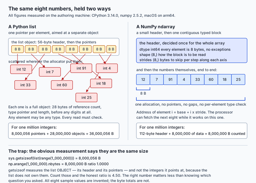
sys.getsizeof measures the list object: a fifty-six-byte header, then one eight-byte pointer per element. It does not measure the integers. It cannot, because the list does not own them — they are a million separate objects sitting somewhere else in memory, and the list only knows where. Count those too and the picture changes:
  the list's pointers                  8,000,056 bytes
  the integers they point at          28,000,000 bytes
  list total                          36,000,056 bytes
  array total                          8,000,000 bytes
  the array is                              4.50x smaller
Twenty-eight bytes for the integer 7. Not eight — twenty-eight, because a Python int is a full object with a reference count, a pointer to its type and a length before you get to any digits at all.
Now the part that costs you money. Here is the same arithmetic — multiply by 2.5, add 1.25 — over those million values, written as a loop and written as an expression, timed five times each on this machine today:
  scale and offset:  2.5 * x + 1.25
    elementwise identical over 1,000,000 elements : True
    loop  ms  [33.9, 30.37, 29.92, 29.66, 29.75]
    array ms  [0.267, 0.243, 0.24, 0.243, 0.23]
    median loop    29.92 ms
    median array   0.243 ms
    speedup        123.2x
The same answer — not close, identical, every one of the million elements compared with == rather than with a tolerance — and a hundred and twenty-three times the speed.
You are three months from writing code that touches millions of numbers. Every image is an array. Every batch of text becomes an array of token identifiers. Every model weight, every gradient, every attention score. If your instinct at that point is “loop over the items and do the thing”, the difference between a two-minute training step and a four-hour one is not your hardware. It is that instinct.
So today NumPy stops being the answer key beside your from-scratch implementations and becomes the subject. And the thing being taught is not a library. It is a change of habit — from loop over the items to express the whole operation on the whole array — and, because this course does not sell things, an honest account of what that change costs you.
The idea in plain language
You have a shopping list and a delivery van.
The shopping list is a Python list. It can hold anything: three apples, a hammer, the word “Tuesday”, another list. Each entry is written on its own scrap of paper and the list is really a stack of notes saying the apples are on shelf four, the hammer is in the shed. To act on an entry you follow the note, find the thing, work out what kind of thing it is, do something to it, and write a new note about the result.
That flexibility is genuinely wonderful and it is why Python is pleasant to write. It is also the entire cost.
The delivery van is a NumPy array. Before it leaves you decide one thing: this van carries eight-kilogram boxes and nothing else. Every box is the same size, they are stacked end to end with no gaps, and the driver does not need to look inside any of them. To act on the load, you do not open boxes one at a time. You say “add one kilogram to every box” and the whole van is handled in one instruction.
The dtype is the decision about what the van carries. The shape is how the boxes are arranged inside it. The strides are how far to step to reach the next box. And the promise those three make together — same type, fixed positions, one block — is what lets the work happen in compiled code instead of in the interpreter.
This analogy will carry the whole lesson, so it is worth naming its two sharp edges now, because both are real and both bite.
The van cannot carry a hammer. Declaring that every box is eight kilograms means a box that would weigh nine cannot be loaded — it wraps round to something small and negative and nobody tells you. That is the dtype section.
The van is loaded once. When you ask for “the boxes in row three” you do not get your own copy of them; you get a hatch onto the same boxes, and anything you do through the hatch happens to the van. That is the views-versus-copies section, and it is where a beginner’s hardest bug lives.
Historical background
There is a temptation, in a section like this, to write a paragraph of dates and names. This lesson is going to decline, and the reason is worth stating openly, because it comes up again every time you read about a tool.
The six sources this lesson cites are listed at the end of the day. Among them are NumPy’s own documentation and its beginner’s guide. Neither page carries a dated account of who built what and when. So rather than reach for a half-remembered version number and a founder’s name, the lesson will not attribute a history it cannot check against something you can also read.
What it can do is show you the history that is still visible in the software, which is more useful anyway. Software carries its past in its interface, and NumPy carries three pieces of it that you will trip over this week.
Two random-number interfaces, one of them marked legacy. Ask the installed library about the older one and it tells you itself:
  Reseed the singleton RandomState instance.

  This is a convenience, legacy function that exists to support
  older code that uses the singleton RandomState. Best practice
  is to use a dedicated ``Generator`` instance rather than
  the random variate generation methods exposed directly in
  the random module.
That is numpy.random.seed’s own docstring, printed from numpy 2.5.2 on the authoring machine. Two interfaces exist because the old one had a design flaw that could not be fixed without breaking everyone: it sets a single global generator that every library in your process shares, so a call you did not write can move your sequence out from under you. The replacement, numpy.random.default_rng(seed), hands you an object you own. Every reproducible number in today’s lab depends on that difference.
A promotion rule that changed at version 2. Add a plain Python 1 to an array of small integers and something has to decide the result’s type. Under NumPy 1 the scalar could drag the array’s type upward; under NumPy 2 it does not. That is why today’s lab pins numpy==2.5.2 and why its test harness checks the major version before asserting anything about dtypes. A tutorial written before that change is not wrong so much as no longer true, and there is no warning on the page to tell you which one you are reading.
A version number in the fourth thousand. The library reports itself as 2.5.2. Whatever else that tells you, it tells you this is not a young project, and that the shape of its interface was argued over by many people for a long time before it settled into something that fits in one lesson.
The deeper history — of matrices, and of the idea that a rectangle of numbers is a function — you met on Days 100 to 102, and Wikipedia’s article on matrices makes the connection in as many words: “Matrices and matrix multiplication reveal their essential features when related to linear transformations, also known as linear maps.” Today is not new mathematics. It is the same mathematics, stored properly.
What it is — and what it is not
An ndarray is a fixed-size, homogeneous, N-dimensional block of numbers, described by a small header.
NumPy’s beginner’s guide states all three constraints plainly. On dimensionality: “the fundamental array class is called ndarray: it represents an ‘N-dimensional array’.” On homogeneity: “All elements of the array must be of the same type of data.” On size: “Once created, the total size of the array can’t change.”
Those are not limitations that were tolerated. They are the entire source of the advantage, and the guide says so: “NumPy shines when there are large quantities of ‘homogeneous’ (same-type) data to be processed on the CPU,” and “by exploiting these characteristics, we can improve speed, reduce memory consumption, and offer a high-level syntax.”
The header carries three attributes you will read a thousand times:
| Attribute | What it says | Example on np.arange(12).reshape(3, 4) |
|---|---|---|
dtype | what every element is, decided once for all of them | int64 — eight bytes each, no exceptions |
shape | how many elements along each axis | (3, 4) — three rows of four |
strides | how many bytes to skip to move one step along each axis | (32, 8) — a row is four int64 along |
Read those strides again, because they are the whole trick. To find element [i, j] the library does not search or follow a pointer. It computes base + 32*i + 8*j and reads eight bytes. The address of every element is arithmetic, which is exactly why a transpose can cost nothing: swap the two strides, hand back a new header over the same bytes, and the array is transposed. Nothing moved.
Now the things it is not, because each of these misreadings produces a specific bug.
It is not a list that happens to be fast. A list is a container of references to objects of any type. An array is a typed region of memory with a description attached. a[0] = "hello" on a list is fine; on an int64 array it raises, and that refusal is the feature.
It is not a matrix. A NumPy array of shape (3, 4) is not automatically a mathematical matrix, and * between two arrays is elementwise multiplication, not the matrix product. @ is the matrix product. Confusing them gives you an array of the wrong shape or — worse — the right shape and the wrong numbers.
It is not exact arithmetic. The dtype is a promise about range and precision, and both can be broken. An int8 holding 127 plus 1 is -128. A float32 above sixteen million cannot tell one integer from the next.
Vectorised does not mean “no loop”. This is the misconception worth carrying away. np.sqrt(a) still visits every element of a. The loop moved from CPython’s bytecode interpreter into compiled C. NumPy’s own broadcasting documentation puts it exactly this way: “Broadcasting provides a means of vectorizing array operations so that looping occurs in C instead of Python.” The loop is not gone. It is not yours.
Why it was created and what problems it solves
Four problems, and each one is measurable rather than rhetorical.
Memory. Twenty-eight bytes per integer against eight is 4.5 times, and that is with int64. Store the same data as int8 where it fits and it is thirty-six times. On a dataset that fits in memory as an array and does not fit as a list, the difference is not “slower”, it is “cannot be done on this machine at all”.
Speed. A hundred and twenty-three times, measured above. The reason is visible if you count what the interpreter does per element: fetch a pointer, follow it, check the object’s type, unbox the double, multiply, add, box the answer into a new float object, store a pointer to it. Seven pieces of bookkeeping around one piece of arithmetic. The array version fetches eight bytes at a computed address, multiplies, adds, stores eight bytes — and because the dtype settled the type question once for the entire array, there is no check to perform.
Expressiveness. This is the one that is undersold. a[a > 5].mean() is nine characters of intent. The loop version is five lines with a counter, an accumulator and an if, and every one of those five lines is somewhere a bug can live. Shorter code is not a matter of taste when the alternative has more places to be wrong.
A shared vocabulary. Every numerical tool in Python speaks ndarray. pandas is a labelled layer over arrays. Matplotlib plots them. scikit-learn takes them. PyTorch and JAX copied the interface on purpose, so that .shape, .dtype, axis=1, broadcasting, boolean masking and argsort mean the same things there. This is not a coincidence and it is not politeness — it is the reason today’s habits transfer to model code without translation.
How it works
The three facts that are really one fact
Fixed dtype, contiguous block, and a shape with strides. They read like three features and they are three faces of one decision.
Because the dtype is fixed, every element is the same width. Because every element is the same width, they can be packed end to end with no gaps. Because they are packed with no gaps, the address of element i is base + i * stride — arithmetic, not a search. And because the address is arithmetic and the type is known, a compiled loop can run over the whole block without consulting Python once.
Take away the fixed dtype and all of it collapses. That is why the first question about any array is a.dtype, and why describe in today’s lab prints all six facts at once:
shape=(3, 4) dtype=int64 itemsize=8 nbytes=96 strides=(32, 8) c_contiguous=TrueMaking arrays without a loop
You will almost never need to build a list and convert it. There is a constructor for the shape you want.
| Call | Gives you | Reach for it when |
|---|---|---|
np.array([1.5, 2.5, 3.5]) | an array from data you have | you already have the numbers |
np.zeros(4) | [0. 0. 0. 0.] | you want an accumulator to fill |
np.ones((2, 3)) | a 2 by 3 block of ones | same, with a different starting value |
np.full(3, 7) | [7 7 7], dtype taken from the 7 | any other constant |
np.arange(0, 10, 2) | [0 2 4 6 8] | you know the step |
np.linspace(0, 1, 5) | [0. 0.25 0.5 0.75 1.] | you know how many you want |
np.eye(3) | the identity matrix from Day 102 | you need a do-nothing transformation |
rng.random(3) | reproducible pseudo-random values | you need randomness you can defend |
The two that get confused are arange and linspace. arange counts in steps and excludes the stop, exactly like Python’s range. linspace takes the number of points you want and includes both ends. Ask for a step, use arange; ask for a count, use linspace.
And the seeding, which matters more than it looks:
rng = np.random.default_rng(104)
rng.random(3)   # [0.83856481 0.69214815 0.21608883]
A second generator built from the same seed gives the same three numbers. A generator is an object you own and pass around, so no other library can move your sequence. That is why every number in today’s lab is the same on your machine as on the authoring machine, and why the lab can assert on specific values rather than on vague properties.
The universal functions
A ufunc is a function that applies elementwise to an array of any shape and returns an array of the same shape.
a = np.array([0.0, 1.0, 4.0, 9.0, 16.0])
np.sqrt(a)     # [0. 1. 2. 3. 4.]
math.sqrt cannot do this. Hand it an array and it raises TypeError: only 0-dimensional arrays can be converted to Python scalars, because it wants one number and is honest about it.
The ones that come up daily are np.abs, np.sqrt, np.exp, np.log, np.sign, np.round and np.maximum. That last one is worth a sentence of its own: np.maximum(x, 0) takes two arrays and compares them elementwise, which makes it the ReLU from Day 102 written as one call. np.max(x) takes one array and reduces it to a single number. The longer name is the elementwise one, and confusing the two is a rite of passage.
Two arrays combine elementwise too, and here is the trap you will hit this week:
left  = np.array([1.0, 2.0, 3.0])
right = np.array([10.0, 20.0, 30.0])
left * right   # [10. 40. 90.]   elementwise
left @ right   # 140.0           the dot product, from Day 103
* is elementwise. @ is the matrix product. In a language with one multiplication symbol this is the single most common source of a silently wrong shape.
Dtypes, and the promise you can break by accident
An int8 holds −128 to 127. Here is 127 plus 1, from a real run:
  np.array([127], dtype=np.int8) + np.array([1], dtype=np.int8)
  gives                -128
  warnings raised      none
No exception. No warning. On numpy 2.5.2, measured rather than assumed, the value simply wraps from the top of the range round to the bottom, and the next line of your program carries on with -128 as though it were the answer.
Where does -128 come from? Two’s complement, eight bits, and one carry that ripples the whole way:
    0111 1111    = 127
  + 0000 0001    =   1
    ---------
    1000 0000    = -128, because the top bit means "negative"
Doubling three int8 values shows how quietly it spreads:
  int8  120 doubled ->   -16   <- wrapped, the true answer is 240
  int8  125 doubled ->    -6   <- wrapped, the true answer is 250
  int8  127 doubled ->    -2   <- wrapped, the true answer is 254
And a plain Python 1 does not rescue you:
np.array([127], dtype=np.int8) + 1 -> [-128] dtype int8Since NumPy 2, the Python scalar takes the array’s dtype rather than the other way round. The array’s promise wins. The fix is to say what you meant — .astype(np.int16) before the arithmetic gives 128 — and to accept that it costs a byte per element, which on a model’s weights is where the whole conversation about half-precision floats comes from.
Floats fail differently, and more quietly. They do not wrap; they stop being able to tell two numbers apart:
  float32 0.1  ->  0.10000000149011612
  float32 16777216 + 1 == 16777216  ->  True
A float32 has twenty-four bits of significand, so at 2²⁴ the gap between neighbouring representable values is exactly 1, and adding 1 lands back where you started. An accumulator in float32 can stop increasing while you are still adding to it, and nothing will tell you.
Boolean masking
This is the single most useful idea in NumPy after broadcasting, and it rests on one fact: a comparison on an array is an array.
Twenty readings from the seeded generator, small enough to check by eye:
[70, 83, 34, 69, 26, 21, 18, 12, 65, 37, 17, 75, 30, 73, 37, 41, 97, 64, 21, 82]Ask whether they are above fifty and you do not get a yes or a no. You get twenty answers:
  readings > 50  ->  [ True  True False  True False False False False  True False False  True
 False  True False False  True  True False  True]
  dtype bool   shape (20,)   size 20
Everything else follows from that:
  mask.sum()   9       True is 1 when summed, so a count is a sum
  mask.any()   True    is anything above 50?
  mask.all()   False   is everything?
  mask.mean()  0.45    what fraction? — a sum divided by n
  readings[mask]  ->  [70, 83, 69, 65, 75, 73, 97, 64, 82]
Four loops with counters and accumulators, replaced by four expressions with nowhere to hide a mistake.
Combining two conditions is where everyone’s first NumPy hour ends:
(readings > 30) & (readings < 70)     # works: 7 readings
(readings > 30) and (readings < 70)   # raises
The failure is not a NumPy shortcoming. It is:
ValueError: The truth value of an array with more than one element is ambiguous. Use a.any() or a.all()and is a control-flow keyword, not an operator. Python evaluates the left side and asks it “are you true?” so it can decide whether to bother with the right side. NumPy cannot redefine that behaviour, because there is no method for Python to call — and an array of twenty answers has no single answer to give. & is an operator, so NumPy defines it to mean elementwise-and, which is what you meant.
The parentheses are not decoration either. & binds tighter than <, so a > 30 & a < 70 parses as a > (30 & a) < 70: a bitwise-and of 30 with every element, then a chained comparison, which calls bool() on an array and raises the identical error for an entirely different reason. Two causes, one message. Bracket every comparison.
Three more tools complete the set. np.where(cond, x, y) is x if cond else y for a whole array. Assignment through a mask — a[a > 90] = 90 — writes only where the mask is True. And fancy indexing takes an array of positions rather than a mask:
readings[[0, 5, 19, 5]] -> [70, 21, 82, 21]Three differences from a mask, all useful: the result takes the shape of the index array, you choose the order, and you may ask for the same element twice. That is how a batch of rows is pulled out of a dataset, and it is what makes the next section’s ranking work.
Axes, and the rule worth memorising
Every aggregation takes an optional axis, and the confusion is universal until you have the rule.
  grid.sum()          66              shape ()
  grid.sum(axis=0)    [12 15 18 21]   shape (4,)
  grid.sum(axis=1)    [ 6 22 38]      shape (3,)
The axis you name is the one that disappears.
A (3, 4) array summed with axis=0 loses the 3 and leaves shape (4,) — one number per column. With axis=1 it loses the 4 and leaves (3,) — one number per row. If you are reading it as “which axis do I want to keep”, you will be off by exactly one, every time, for the rest of your career.
keepdims=True holds the shape open — (3, 1) instead of (3,) — which is precisely what you need when the result has to broadcast back against the array it came from, as in normalising every row to sum to one.
And np.newaxis turns a row into a column so that broadcasting can pair everything with everything:
  v[:, np.newaxis] shape (3, 1)
  v[np.newaxis, :] shape (1, 3)
  v[:, None] - v[None, :]:
    [ 0. -1. -2.]
    [ 1.  0. -1.]
    [ 2.  1.  0.]
Shape (3, 3) — every difference of every pair, in one line, no loop over pairs. That line is how a whole distance matrix gets built, and it is also one of the three ways to run out of memory, which the closing section returns to.
Views versus copies
Here is the bug. Read it slowly, because when it happens to you it will happen a hundred lines away from the cause.
  original:
    [0 1 2 3]
    [4 5 6 7]
    [ 8  9 10 11]

  row_one = original[1]        ->  [4 5 6 7]
  shares memory: True
  row_one[0] = 999

  the ORIGINAL now reads:
    [0 1 2 3]
    [999   5   6   7]
    [ 8  9 10 11]
Nothing was copied, so nothing was protected. NumPy’s own beginner’s guide is explicit about the difference from a list: “slice indexing of a list copies the elements into a new list, but slicing an array returns a view: an object that refers to the data in the original array. The original array can be mutated using the view.” And it does not present this as a footnote: “Views are an important NumPy concept! … modifying data in a view also modifies the original array!”
.copy() breaks the link, and after that the two arrays are strangers.
Which operations give which? There is a pattern, and it is better than the list:
| Expression | View or copy |
|---|---|
a[1], a[:, 1], a[0:2, 1:3] | view |
a.T, a.reshape(4, 3), a.ravel() | view |
a[a > 5] (boolean mask) | copy |
a[[0, 2]] (fancy index) | copy |
a.copy(), a.flatten(), a + 0 | copy |
If the elements you asked for are evenly spaced, a stride can describe them and you get a view. If they are not, NumPy has no choice but to copy. Which means the cheap operations are the dangerous ones, and the expensive ones are safe — the opposite of the intuition most people arrive with.
Note the near-identical pair in that table: ravel() returns a view when it can, flatten() always copies. Two words for one job and opposite behaviour. When you are unsure, np.shares_memory(a, b) answers the question directly.
Sorting, and why you almost always want argsort
  scores          [5. 1. 9. 3.]
  np.sort(scores) [1. 3. 5. 9.]   the values, in order
  np.argsort      [1 3 0 2]       the POSITIONS, in order
argsort answers “which element would come first, then which”. scores[np.argsort(scores)] rebuilds the sorted values, so nothing is lost by taking the indices — but plenty is lost by taking the values.
When the rows mean something — an article, a customer, a token, a candidate answer — the sorted scores are useless on their own. You need to know which row scored what. That is why argsort is the one to reach for, and it is why Day 103’s search becomes one line today:
  all six similarities, from one matrix-vector product and one
  norm along axis=1 -- no loop over articles:
    roast-chicken        0.369119
    slow-cooker-stew     0.360302
    marathon-plan        0.901082
    race-day-nutrition   0.903482
    household-budget     0.041013
    storm-bulletin       0.102533

  np.argsort(sims)          [4, 5, 1, 0, 2, 3]   <- worst first
  reversed, first 3         [3, 2, 0]            <- best first

  top 3:
    1. race-day-nutrition   0.903482
    2. marathon-plan        0.901082
    3. roast-chicken        0.369119

  margin between first and second: 0.002400
Day 103 computed those six similarities one article at a time. Today it is matrix @ query for all the dot products at once, and np.linalg.norm(matrix, axis=1) for one length per row. Same arithmetic, same answer, no loop over articles.
Note also that the lab reports the margin rather than announcing a winner. A gap of two thousandths between first and second is not evidence of much, and a system that hides that from you is worse than one that shows it.
One refinement you will meet in model code, where the catalogue has a hundred thousand rows and you want ten: np.argpartition does not sort everything. It only guarantees that the k best land in the first k places, in no particular order, which you then sort. On six articles that saves nothing. On a hundred thousand it is the difference between sorting them all and not.
nan, and the comparison that surprises everybody
  np.nan == np.nan   ->  False
  np.nan != np.nan   ->  True
Not a NumPy decision. IEEE-754 says nan compares unequal to everything including itself, because nan means not a number — the result of 0/0, of the square root of a negative, of a reading that was never taken. Two unknowns are not known to be the same unknown.
So this does not work, and fails silently:
  a = [ 1.  2. nan  4.]
  a == np.nan   ->  [False False False False]
Every answer False, including for the element that is nan. A filter written that way finds nothing and reports success. np.isnan(a) asks about the bit pattern instead, and finds it.
And one hole poisons the whole aggregate, deliberately:
  a.sum()        nan          np.nansum(a)   7.0
  a.mean()       nan          np.nanmean(a)  2.3333333333333335
  a.max()        nan          np.nanmax(a)   4.0
The plain versions are not broken. They are telling you, loudly and at the point where it starts to matter, that a value is missing. Reaching for the nan-prefixed version is a decision to ignore that, and it should be a decision rather than a reflex — because 2.333... is the mean of the three readings you have, and not the mean of the four you wanted.
An everyday analogy
Back to the van, and now it can carry the whole day.
Loading. A shopping list of scraps of paper against a van of identical eight-kilogram boxes. Making the list is effortless and heterogeneous; loading the van requires you to decide what it carries. That decision is the dtype, and it is the price of admission.
Working. With the shopping list you walk the shelves: read a note, find the item, work out what it is, do the thing, write a new note. With the van you tell the driver “add one kilogram to every box” and the whole load is handled at once. The work per box did not change; the walking did. That is the loop moving from Python into C, and it is why “vectorised” does not mean “no loop”.
The weight limit. A box that would weigh nine kilograms cannot be loaded. It does not bounce; it silently comes out weighing minus seven, and the manifest still balances. That is int8 at 127. The van keeps the promise you made even when keeping it produces nonsense.
The hatch. Ask for “the boxes in row three” and you are handed a hatch onto them, not a copy of them. Anything you do through the hatch happens to the van. That is a slice, and .copy() is the request to actually unload them onto a pallet of your own.
The manifest. Sorting the boxes by weight gives you a list of weights and loses which box was which. Sorting the manifest numbers by weight keeps the identity. That is argsort, and it is why a search returns indices.
The box marked “contents unknown”. It is not empty and it is not zero. Any total that includes it is honestly unknown, and a driver who quietly left it out of the total and told you the van weighed less than it does would be worse than useless. That is nan, and that is why mean() returns nan rather than guessing.
Where the analogy breaks, and it is worth knowing: a real van’s boxes are physically separate, and array elements are not — they are one continuous stretch of memory that the shape and strides merely describe. That is why the same bytes can be a (3, 4) array in the morning and a (4, 3) array after a transpose with nothing having moved. No arrangement of real boxes does that.
Examples in practice
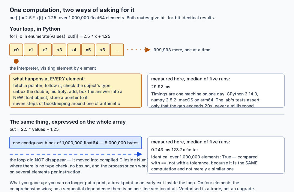
Today’s lab implements three operations twice — once as an explicit Python loop, once as a NumPy expression — and asserts they agree exactly before timing either. That order matters. A speed comparison between two things that give different answers is not a comparison of anything.
Here is the full measured result from one run:
  scale and offset:  2.5 * x + 1.25
    elementwise identical over 1,000,000 elements : True
    median loop    29.92 ms
    median array   0.243 ms
    speedup        123.2x

  square root:       math.sqrt(x)  vs  np.sqrt(a)
    elementwise identical over 1,000,000 elements : True
    median loop    34.80 ms
    median array   0.260 ms
    speedup        134.0x

  clip:              hold x inside [0.25, 0.75]
    elementwise identical over 1,000,000 elements : True
    median loop    27.69 ms
    median array   0.261 ms
    speedup        106.2x
Three things about this measurement, all of them the point.
Identical, not close. 2.5, 1.25, 0.25 and 0.75 are exactly representable in binary. Each element goes through the same operations in the same order on the same sixty-four bits. There is no room for a difference and none appears, so the lab compares with == rather than with a tolerance. Using a tolerance would have hidden the very fact being demonstrated.
Five runs, and all five shown. A single timing is noise. The median is reported because one unlucky run — the operating system deciding to do something else for thirty milliseconds — drags a mean around and leaves a median alone.
One machine, one day. Apple Silicon, macOS 26.5.2, CPython 3.14.0, numpy 2.5.2. Your figures will differ. Which is exactly why the lab’s tests assert that the speedup exceeds twenty, and never assert a millisecond. A test that asserted 123x would fail on a slower laptop and teach the reader that the suite is unreliable rather than that their laptop is different.
And now the finding that came out of building this lesson and was not planned.
The lab’s roots_loop uses math.sqrt(x) rather than x ** 0.5. That looks like a stylistic choice. It is not:
  over 1,000,000 values, compared with np.sqrt:
    math.sqrt(x)  disagrees on      0 of them
    x ** 0.5      disagrees on  1,390 of them

  the first disagreement, at index 781:
    x           0.6541050943199698
    x ** 0.5    0.808767639263571
    np.sqrt(x)  0.8087676392635711
    difference  1.110e-16
One value in seven hundred, always by one unit in the last place. IEEE-754 requires the square-root operation to be correctly rounded — there is exactly one right answer for every input — and both math.sqrt and numpy.sqrt use the hardware instruction that obeys that. pow(x, 0.5) is a general power routine with no such requirement, because computing an arbitrary power exactly is a much harder problem than computing a square root.
So “the vectorised version gives the same answer” is a claim about the operation, not about anything that would agree in exact arithmetic. If a vectorised rewrite of yours suddenly needs a tolerance it did not need before, that is the first thing to check — and it is worth reading rather than widening.
Implications: security, privacy, performance, scalability, and cost
Security. Silent integer overflow is not a curiosity; it is a class of exploitable bug with decades of history behind it. A value that was supposed to be too large becomes negative, the “is it too big?” check passes, and the code proceeds on an assumption that is now false. Python itself is immune, because a Python int grows to whatever size it needs. The moment you put data into a fixed-width array you have opted into a promise about range, and NumPy will keep that promise even when keeping it produces nonsense. Check a.dtype first whenever a number looks impossible.
Privacy and the shape of a leak. A view shares memory. If a function hands a caller data[0:100] believing it has given them a copy of the first hundred rows, it has given them a window onto the array — and anything they write lands in yours. Returning a view is a decision, not an accident to be discovered later.
Performance. Two orders of magnitude on elementwise work, measured. But the fixed cost of a NumPy call — resolve the dtypes, work out the output shape, allocate it — is real, and on small arrays it is the whole bill. On four elements the list comprehension won on this machine, at 0.108 microseconds against 0.325. The crossover here is in the low hundreds of elements. Measure yours rather than believing this paragraph.
Scalability. Vectorising trades time for memory, and the trade is not always favourable. x[:, None] - x[None, :] allocates n² elements whether you need them all or not:
    all pairs of   1,000 points, float64 :       0.01 GB
    all pairs of  10,000 points, float64 :       0.80 GB
    all pairs of  30,000 points, float64 :       7.20 GB
    all pairs of 100,000 points, float64 :      80.00 GB
The elegant one-line distance matrix is the reason the process died. The ugly loop that handles a thousand at a time is slower and finishes.
Cost. Dtype is money. A million float64 values are 8 MB; the same values as float32 are 4 MB and as float16 are 2 MB. On model weights that is the difference between a card you can rent and one you cannot. It is also exactly the trade the float32 blind spot describes — you are buying capacity with precision, and it is worth knowing which precision you sold.
Alternatives: free, open source, and commercial
NumPy is the one that was actually run for this lesson, on this machine, at version 2.5.2. Everything below it is described from its documentation, and no output from any of them is reproduced here, because none of them were installed. That distinction is the difference between a description and a claim.
NumPy — free, open source, BSD 3-Clause. The baseline, and the one to learn first. Choose it whenever your data fits in memory on one machine and you are working on a CPU, which covers the overwhelming majority of data work and all of this course for the next several weeks. How to use it: pip install numpy, then import numpy as np, and everything in today’s lab. Concrete example: np.argsort(similarities)[::-1][:3] returning the three nearest articles, which is the whole of a semantic search’s ranking step. There is no paid tier; there is no tier at all.
PyTorch — free, open source. The axis it extends NumPy along is automatic differentiation: a torch.Tensor records the operations performed on it so that gradients can be computed backwards through them, which is the machinery every trained model needs. Choose it when you are training something. The interface was copied from NumPy deliberately — .shape, .dtype, axis (spelled dim), broadcasting, boolean masking and argsort all carry across — so today’s habits are the habits you will use there. Free to use; the money in that ecosystem is in the hardware and the hosted training, not the library.
JAX — free, open source. Its axis is compilation and accelerators: the same array interface, plus a just-in-time compiler that fuses your expression into a single optimised kernel, plus function transformations for gradients and for vectorising a function over a batch automatically. Choose it for research code that must be fast and mathematical at the same time. The cost is a discipline NumPy does not impose: arrays are immutable, so a[0] = 1 is replaced by a.at[0].set(1), and a habit you form today has to be unlearned there.
CuPy — free, open source. Its axis is the GPU, and only that. It aims to be a drop-in replacement for NumPy’s interface where import numpy as np becomes import cupy as cp and the arrays live in graphics-card memory. Choose it when you have array code that already works, a GPU, and no desire to rewrite anything. The catch is honest and worth stating: it needs a compatible GPU and its drivers, and moving data to and from the card costs time that can erase the gain on small work.
Dask — free, open source. Its axis is out-of-core and distributed: a Dask array presents the NumPy interface over data that is split into chunks, which may be larger than memory or spread across machines, and it builds a task graph rather than computing immediately. Choose it when the honest answer to “does it fit in memory” is no. The cost is that the mental model changes — nothing happens until you ask for a result — and that a poorly chosen chunk size can be slower than doing nothing clever at all.
pandas — free, open source, and not a competitor. It is the labelled layer above NumPy: a DataFrame is a set of columns, most of them backed by NumPy arrays, with names on the columns and an index on the rows. Choose it when your data has headings and mixed types — a CSV, a table from a database — and when you want to group by something. Underneath, the vectorised thinking is identical, which is why today comes before it.
Two commercial notes, stated qualitatively because this course does not quote prices. Hardware vendors ship tuned linear-algebra libraries that NumPy can be built against, and a build linked to one of those can be substantially faster on matrix work than a generic build with no change to your code. And the managed notebook and training platforms sell you access to machines with GPUs; what they sell is the hardware and the convenience, not the array library, which remains free everywhere.
What was actually run here: NumPy 2.5.2 only. PyTorch, JAX, CuPy, Dask and pandas were not installed and produced no output for this lesson.
Comparison with related concepts
| Concept | What it is | How it differs from today’s subject |
|---|---|---|
Python list | a container of references to objects of any type | heterogeneous, resizable, no dtype and no shape; a slice copies |
Python array.array | a typed, one-dimensional sequence from the standard library | has a dtype but no shape, no strides, no broadcasting, no ufuncs |
ndarray | a fixed-size homogeneous N-dimensional block plus a header | the subject of today |
pandas DataFrame | labelled columns, mostly backed by ndarrays | adds names, an index and mixed column types on top of arrays |
torch.Tensor | an ndarray-like object that records its own history | adds autograd and device placement; interface deliberately familiar |
And five pairs that are commonly confused, each with the distinction that resolves it:
| Confused pair | The distinction |
|---|---|
* and @ | * is elementwise; @ is the matrix product from Day 101 |
np.max and np.maximum | np.max reduces one array to a number; np.maximum compares two arrays elementwise |
ravel and flatten | both flatten; ravel returns a view when it can, flatten always copies |
np.sort and a.sort() | np.sort returns a new array; the method sorts in place and returns None |
a == np.nan and np.isnan(a) | the first is always False; only the second finds anything |
When to use it — and when not to
Reach for the array when the data is homogeneous, the operation is the same for every element, and there is enough of it that the per-call overhead disappears — which in practice means more than a few hundred elements. Reach for it also when the alternative loop would need three nested levels and a counter, because expressiveness is worth as much as speed and is easier to verify.
Now the honest half, which most introductions omit.
When the array is small. Measured on this machine, on four elements: the list comprehension at 0.108 microseconds, the NumPy call at 0.325. Every NumPy call has to resolve dtypes, work out the output shape and allocate it before any arithmetic happens, and on four elements that setup is the entire bill. If you are calling a function on small arrays in a tight outer loop, NumPy can make your program slower.
When each step depends on the last. A running balance, floored at zero:
    start 100, changes -30, +50, -200, +20, floored at zero
    the honest loop  [70.0, 120.0, 0.0, 20.0]
    np.cumsum route  [70.0, 120.0, 0.0, 0.0]
Different answers, and the loop’s is the right one — step four depends on the floor applied at step three, and a cumulative sum cannot know that. Sequential dependence is the clearest signal that the loop should stay.
When memory would blow up. The pairwise table again. At a hundred thousand points, x[:, None] - x[None, :] needs 80 GB. The slower loop that processes a thousand at a time finishes.
When the loop is simply clearer and the data is small. A dozen configuration values, a handful of records, a one-off script. Rewriting that as array expressions costs reading time and buys microseconds nobody will ever notice. Vectorising is a trade, not an upgrade, and a tool you can only argue for is a tool you do not understand yet.
Where this goes next in AI work
Every tensor library you will meet copied NumPy’s interface on purpose. torch.Tensor and jax.numpy use the same .shape, the same .dtype, the same broadcasting rules, the same boolean masking, the same argsort. That is not a coincidence — it is a deliberate decision by their authors to let people arrive already knowing how to hold the thing.
Which means the three habits from today are the daily vocabulary of model code, not a stepping stone to it. Batching is shape work: (batch, sequence, features), and getting axis right is the difference between averaging over the batch and averaging over time. Masking is how a model ignores padding tokens, how attention is stopped from looking ahead, and how a loss is computed over only the positions that count — all of it boolean arrays and np.where, spelled slightly differently. And top-k selection is argsort or argpartition: the last step of a search, the sampling step of a language model, the retrieval step of anything that answers questions from documents.
When you write your first PyTorch training loop, the parts that will confuse you will not be the parts you learned today.
Knowledge check
Eight questions in the quiz for this day, including one on why and fails on arrays and one on views versus copies. Take it before the lab if you want to find out what you already believe, and after the lab if you want to find out what you now know.
Hands-on exercise
Open the day’s lab, “Stop Writing the Loop”, and work through starter/00_brief.md.
The spine is exercise 1: ten functions, three of them written twice — once as an explicit Python loop, once as a NumPy expression — with a test that compares the two over a million elements using == rather than a tolerance. Then exercises 2 to 7 are forty-two predictions you make before running anything: memory ratios, the int8 wrap, mask counts you can check by eye against twenty printed readings, axis shapes, view-versus-copy outcomes, and the nan results.
Install first, from the lab directory:
python3 -m venv .venv
.venv/bin/pip install -r requirements/requirements.txt
.venv/bin/python3 -c "import numpy; print(numpy.__version__)"
Then work, checking yourself as you go:
.venv/bin/pytest starter -qExpected output
On an untouched checkout:
1 passed, 70 skippedA skip means “not attempted”. A failure means “attempted and wrong”, and prints both your answer and the real one. When it says 71 passed, you are finished.
The full harness, run from the lab directory, ends like this:
80 checks, 0 failure(s).and exits 0. Three blocks from the reference scripts are worth recognising when you meet them. The measurement that appears to disprove the lesson:
  sys.getsizeof(list)      8,000,056 bytes
  array.nbytes             8,000,000 bytes
  ratio                       1.0000
The silent wrap:
  np.array([127], dtype=np.int8) + np.array([1], dtype=np.int8)
  gives                -128
  warnings raised      none
And the error you will meet on your own within a week:
ValueError: The truth value of an array with more than one element is ambiguous. Use a.any() or a.all()Validate your work
bash tests/run_tests.sh; echo "exit=$?"prints80 checks, 0 failure(s).andexit=0..venv/bin/pytest examples -q -p no:cacheproviderprints107 passed..venv/bin/pytest starter -q -p no:cacheproviderprints71 passedonce you have finished.- Each of the seven reference scripts ends with
every assertion held. find . -path ./.venv -prune -o -type d -name '__pycache__' -printprints nothing after a full run.
Troubleshooting
ValueError: The truth value of an array... — three separate causes and the same message. You used and/or instead of &/|; or you left the parentheses off, so & bound tighter than <; or you put an array inside an if. The lab’s troubleshooting.md separates all three.
ModuleNotFoundError: No module named 'vectorize' — you are in the wrong directory. The scripts in examples/ import from beside themselves, so run them from inside examples/. The pytest suites are the other way round: run those from the lab directory.
Your filter for missing values finds nothing — you wrote a == np.nan. Use np.isnan(a).
An array you were not looking at changed — you have a view. Check with np.shares_memory(a, b) and call .copy() when you mean to own the result.
Your speedup is much smaller than the captured one — expected, and not a failure. Check you are timing the loop over a list and the vectorised version over an array; looping over an ndarray with a Python for is slower than looping over a list, because every element must be boxed on the way out.
Common mistakes
Trusting sys.getsizeof. It measures the object you handed it and not the objects it points at. This is the mistake the lesson opens with, deliberately.
Comparing a slow loop against a fast array. The lab’s loops allocate their output up front rather than appending, because a rigged comparison teaches nothing. If you write the loop badly to make NumPy look good, you have measured your own bad loop.
Asserting a timing. A test that says “this took under 5 ms” fails on someone else’s machine and teaches them that the suite is unreliable. Assert the shape of the gap.
Using x ** 0.5 in the loop and np.sqrt in the array version. Different operations, and one test in the lab will catch you. Use math.sqrt.
Reading axis as “the one I keep”. It is the one that disappears.
Forgetting that a boolean mask copies and a slice does not. The expensive operation is the safe one, which is the opposite of the intuition most people bring.
Practice assignment
Take a dataset of your own — a CSV of anything, or one you generate with a seeded default_rng — and write the same analysis twice.
First as loops: read the rows, filter on two conditions, compute a mean of one column over the survivors, and find the five rows with the largest value in another column. Use no NumPy at all.
Then as array expressions: one boolean mask combining both conditions with &, one masked mean, one argsort for the top five.
Then do three things with the pair, and write down the answers rather than merely thinking them.
Prove they agree. Not “look similar” — assert it. Decide honestly whether == is right here or whether a tolerance is genuinely needed, and if you reach for a tolerance, work out why the two routes differ before you choose the number.
Time both, properly. Five runs each, report the median and show the spread, and state your machine and versions beside the figures. Then write one sentence you would be willing to defend in a code review about what the ratio means and what it does not.
Find your crossover. Cut the dataset to 10 rows, 100, 1,000, 10,000 and time both at each size. Somewhere the lines cross. Report where, and then explain why the crossover moves when you make the per-element operation more expensive — swap the multiply for np.exp and measure again.
The deliverable is a short note with those three answers, the numbers that support each, and one honest sentence about anything that surprised you. If nothing surprised you, you probably did not measure carefully enough.
Extension challenge
Build a top-k semantic search over a hundred thousand items, and make every step of it defensible.
Generate the catalogue with a seeded generator: a hundred thousand rows of, say, sixty-four features each. That is a (100000, 64) float64 array — work out what it costs in memory before you allocate it, and check your arithmetic against a.nbytes afterwards.
Then:
- Score every row against a query in one expression. No loop over rows. Use
axis=1for the norms andkeepdimsif you need the result to broadcast back. - Take the top ten two ways —
argsortandargpartition— and confirm they give the same ten. Time both, and predict the ratio from what each has to do before you measure it. - Cut the memory in half. Convert the catalogue to float32 and repeat. Then answer the question that matters: did any of the top ten change, and if so, by how much did the scores move? You now have a concrete instance of the precision-for-capacity trade the lesson described in the abstract.
- Break it on purpose. Put a
naninto one row of the catalogue. Watch whatargsortdoes with it — where does it sort to, and does your top ten quietly change? Then decide what your code should do about a missing row, and implement that rather than the first thing that makes the symptom go away. - Now try to allocate the full pairwise similarity matrix between all hundred thousand items. Work out the size first. Do not run it. Write down what you would do instead, and what the chunk size would depend on.
The last two are the ones worth your time. Anyone can make an array fast. Knowing what it does when the data is wrong, and knowing when the elegant line is the one that kills the process, is the part that makes you someone people trust with a pipeline.
Quiz
Q1. You write `(readings > 30) and (readings < 70)` on a NumPy array and get `ValueError: The truth value of an array with more than one element is ambiguous`. Why?
- `and` is a Python keyword rather than an operator, so it asks the left array for a single True or False, and twenty answers cannot give one
- NumPy has not implemented `and` for arrays yet; a future version will
- `and` only works on lists, so the arrays must be converted with `.tolist()` first
- The two comparisons produce arrays of different lengths, which cannot be combined
Show answer
Answer: A. `and` is a Python keyword rather than an operator, so it asks the left array for a single True or False, and twenty answers cannot give one
This is not something NumPy could fix if it wanted to. `and` is control flow: Python evaluates the left operand and asks whether it is truthy so it can decide whether to bother evaluating the right one. There is no method for Python to call on the array — it calls `bool()`, and an array of twenty answers has no single answer, so it refuses rather than guessing. `&` IS an operator, so NumPy defines it to mean elementwise-and, which is what you meant. Option 1 is the reassuring misreading; option 2 is backwards, since converting to lists loses the very thing that makes the expression worth writing; option 3 is wrong because both comparisons are made on the same array and so produce identical shapes. Note the error message names its own escape routes, `.any()` and `.all()`, which are the two questions that DO have a single answer.
Q2. `row = grid[1]` on a 2-D array, then `row[0] = 999`. What happens to `grid`?
- Nothing — `grid[1]` returned a copy of row one, exactly as list slicing would
- `grid[1, 0]` becomes 999, because a slice returns a view onto the same memory
- NumPy raises an error, because views are read-only
- `grid` is unchanged but `row` is now detached from it, so later reads diverge
Show answer
Answer: B. `grid[1, 0]` becomes 999, because a slice returns a view onto the same memory
Slicing an array returns a *view*: a new header over the same bytes. NumPy's own beginner's guide draws the contrast explicitly — "slice indexing of a list copies the elements into a new list, but slicing an array returns a view ... The original array can be mutated using the view" — and adds "modifying data in a view also modifies the original array!". Option 0 is the intuition you bring from lists and it is exactly what makes this bug hard: the code that breaks is nowhere near the code that caused it. Option 2 is wrong; views are perfectly writable, which is the whole problem. The useful pattern is that if the elements you asked for are evenly spaced, a stride can describe them and you get a view — slices, transposes, reshapes, `ravel`. If they are not, NumPy has no choice but to copy — boolean masks, fancy indexing, `flatten`. So the cheap operations are the dangerous ones. `.copy()` breaks the link, and `np.shares_memory(a, b)` answers the question directly.
Q3. `np.array([127], dtype=np.int8) + 1` — what does it give, and what happens on the way?
- `[128]` as int64, because the plain Python 1 widens the result
- `[127]`, because NumPy clamps rather than wrapping
- It raises `OverflowError`, which is how Python normally reports this
- `[-128]` as int8, silently: no exception and, on numpy 2.5.2, no warning either
Show answer
Answer: D. `[-128]` as int8, silently: no exception and, on numpy 2.5.2, no warning either
An int8 holds -128 to 127. In two's complement, 127 is 0111 1111 and adding 1 carries all the way into the sign bit to give 1000 0000, which reads as -128. Nothing raises, and this was measured rather than assumed: the lab captures the warning list and asserts it is empty on numpy 2.5.2, so that if a future release started warning, the suite would say so rather than let the lesson quietly go stale. Option 0 was closer to true under NumPy 1; since NumPy 2 a Python scalar takes the array's dtype rather than dragging it upward, which is why the lab pins the version and checks the major number before asserting anything about dtypes. Option 1 describes saturating arithmetic, which some image libraries do and NumPy does not. Option 2 describes Python's own integers, which have no maximum at all — the hazard is acquired the moment you put data into a fixed-width array. The fix is to say what you meant: `.astype(np.int16)` before the arithmetic gives 128, at a cost of one extra byte per element.
Q4. `grid` has shape `(3, 4)`. What shape does `grid.sum(axis=1)` have?
- `(4,)` — axis 1 has length 4, so four numbers come out
- `(3,)` — the axis you name is the one that disappears, leaving one number per row
- `(3, 4)` — summing does not change the shape unless you ask it to
- `(1, 4)` — the summed axis is kept at length one
Show answer
Answer: B. `(3,)` — the axis you name is the one that disappears, leaving one number per row
The rule is: **the axis you name is the one that disappears.** Naming `axis=1` collapses the 4 and leaves shape `(3,)` — one total per row, which for `np.arange(12).reshape(3, 4)` is `[6, 22, 38]`. Option 0 is the single most common error in the whole topic, and it comes from reading `axis` as "the axis I want to keep"; anyone reading it that way is wrong by exactly one, every time. Option 3 describes what you get with `keepdims=True`, which is genuinely useful and is a different request: it holds the collapsed dimension open at length 1 so the result can broadcast back against the array it came from, which is exactly what normalising every row to sum to one requires. The same rule governs `min`, `max`, `mean` and `np.linalg.norm`, which is why `np.linalg.norm(matrix, axis=1)` on a 6 by 4 catalogue gives six lengths rather than four.
Q5. You have a million integers in a Python list and the same million in an int64 array. `sys.getsizeof(list)` is 8,000,056 and `array.nbytes` is 8,000,000. What should you conclude?
- That the memory advantage of arrays is a myth for integers, and only applies to floats
- That `sys.getsizeof` measured the list object and its pointers, not the integer objects the list points at
- That the array is inefficient here, since it saved only 56 bytes
- That the two are equal because CPython caches all integers, so the list stores no duplicates
Show answer
Answer: B. That `sys.getsizeof` measured the list object and its pointers, not the integer objects the list points at
`sys.getsizeof` reports the size of the object you hand it: for a list, a 56-byte header plus one 8-byte pointer per element. It cannot include the integers, because the list does not own them — they are a million separate objects elsewhere in memory. Each is 28 bytes on CPython 3.14, since a Python int carries a reference count, a type pointer and a length before any digits. Count them and the honest total is 36,000,056 against 8,000,000, a ratio of 4.5. Option 3 contains a real fact used wrongly: CPython does cache the integers from -5 to 256, but `range(1_000_000)` builds a fresh object for every value above that, and the lab verifies there are a million distinct objects rather than assuming it. Options 0 and 2 both take a wrong measurement at face value, which is the actual lesson here — the right number matters less than knowing which question you asked.
Q6. You need the three nearest articles to a query from six similarity scores. Which is the right tool?
- `np.sort(scores)[::-1][:3]`, which gives the three best scores
- `np.argsort(scores)[::-1][:3]`, which gives the positions of the three best
- `scores.sort()`, which returns the ranking
- `np.max(scores)` three times, removing the winner each time
Show answer
Answer: B. `np.argsort(scores)[::-1][:3]`, which gives the positions of the three best
`argsort` returns the indices that would sort the array, and the indices are the entire answer: when the rows mean something — an article, a customer, a token, a candidate — knowing that the best score was 0.903 tells you nothing without knowing which row it came from. `scores[np.argsort(scores)]` reconstructs the sorted values, so nothing is lost by taking indices, while option 0 loses the identity permanently. Option 2 is a real trap worth knowing: the method `a.sort()` sorts IN PLACE and returns `None`, so that line assigns nothing and quietly reorders the array you were holding — a different behaviour from `np.sort(a)`, which returns a new array and leaves the original alone. Option 3 works and is the loop you are learning not to write. At scale there is a better relative still: `np.argpartition` only guarantees the k best land in the first k places, which on a hundred thousand rows is the difference between sorting them all and not.
Q7. An array contains `[1.0, 2.0, nan, 4.0]`. You write `a[a == np.nan]` to find the missing value. What happens?
- It returns the nan, since the comparison matches it
- It raises a ValueError, because nan cannot be compared
- It returns an empty array, because nan compares unequal to everything including itself
- It returns all four elements, because any comparison with nan is True
Show answer
Answer: C. It returns an empty array, because nan compares unequal to everything including itself
IEEE-754 specifies that nan compares unequal to everything, itself included — `np.nan == np.nan` is False. The reason is not arbitrary: nan means *not a number*, so two of them are two unknowns, and two unknowns are not known to be the same unknown. The consequence is that this filter finds nothing and reports success, which is worse than raising, and it is why `np.isnan(a)` exists: it asks about the bit pattern instead of about equality. The same rule explains why `a.mean()` on that array returns nan rather than 2.333 — the nan propagates through every arithmetic operation it touches. That is a feature, not a bug: it tells you loudly, at the point where it matters, that a value is missing. `np.nanmean` gives 7/3, the mean of the three readings that exist, and reaching for it should be a decision rather than a reflex, because the mean of the three you have is not the mean of the four you wanted.
Q8. When is a Python loop the better choice over a vectorised NumPy expression?
- Never — vectorising is always faster and always clearer
- Only when NumPy is unavailable, since the vectorised form is otherwise strictly better
- When the array is small, when each step depends on the previous one, or when the vectorised form would allocate more memory than you have
- When the data is floating point, since integer arrays are the only ones NumPy handles well
Show answer
Answer: C. When the array is small, when each step depends on the previous one, or when the vectorised form would allocate more memory than you have
All three of those were measured rather than asserted. **Small arrays:** every NumPy call resolves dtypes, works out the output shape and allocates it before any arithmetic; on four elements that setup is the whole bill, and on the authoring machine the list comprehension won at 0.108 microseconds against 0.325. **Sequential dependence:** a running balance floored at zero cannot be written as one expression, because step four depends on the floor applied at step three — `np.cumsum` gives a different and wrong answer, and the lab asserts that it differs. **Memory:** the elegant one-line pairwise table `x[:, None] - x[None, :]` allocates n squared elements, which at a hundred thousand points is 80 GB; the ugly loop that handles a thousand at a time is slower and finishes. Option 0 is the sales pitch and this course does not sell things. Vectorising is a trade — speed and expressiveness for the ability to put a print, a breakpoint or an early exit inside the loop — and a tool you can only argue for is a tool you do not understand yet.
Glossary
- ndarray
- NumPy's array type: a fixed-size, homogeneous, N-dimensional block of values described by a small header. NumPy's own beginner's guide states all three constraints — it "represents an N-dimensional array", "all elements of the array must be of the same type of data", and "once created, the total size of the array can't change". Those constraints are not tolerated limitations; they are the entire source of the speed and memory advantage, because they are what allow the values to be packed in one block and read without a per-element type check.
- dtype
- The data type shared by every element of an array, recorded once in the header rather than per element. It fixes the width of every element, which is what makes the block contiguous and the address of element i computable as base plus i times stride. It is also a promise about range and precision that can be broken by accident: an int8 holds -128 to 127 and wraps silently past either end, and a float32 has 24 bits of significand and cannot distinguish 16,777,216 from 16,777,217. Check a.dtype first whenever a number looks impossible.
- shape
- A tuple of non-negative integers giving the number of elements along each axis — NumPy's guide defines it as exactly that. A (3, 4) array holds twelve values arranged as three rows of four, in one block. The shape is a description of how to read the block, not a description of how it is stored, which is why reshaping and transposing can cost nothing.
- stride
- How many BYTES to skip to move one step along an axis. A (3, 4) array of int64 has strides (32, 8): one column across is one 8-byte element, one row down is four of them. Strides are what turn indexing into arithmetic rather than a search, and swapping two of them is all a transpose has to do — which is why a transpose copies nothing.
- contiguous
- Laid out in one unbroken run of memory, so that consecutive elements sit at consecutive addresses. C-contiguous means the last axis varies fastest — rows laid end to end; F-contiguous means the first does. A transpose of a C-contiguous array is F-contiguous over the same bytes. Contiguity is what lets the processor fetch the next values while it is still working on the current one, and it is inseparable from the fixed dtype: without a fixed width there is no way to pack without gaps.
- Universal function
- A NumPy function that applies elementwise to an array of any shape and returns an array of the same shape — np.sqrt, np.exp, np.abs, np.sign, np.maximum and the arithmetic operators are all ufuncs. Usually shortened to ufunc. The equivalent list comprehension gives the same answer and takes roughly a hundred times as long, because the ufunc's loop is compiled rather than interpreted. math.sqrt is not a ufunc and raises TypeError when handed an array.
- Vectorisation
- Expressing an operation on a whole array at once rather than element by element in Python. The loop does not disappear — NumPy's broadcasting documentation puts it exactly: "Broadcasting provides a means of vectorizing array operations so that looping occurs in C instead of Python." What you gain is speed and expressiveness; what you give up is the ability to put a print, a breakpoint or an early exit inside the loop, and the option of a step that depends on the one before it.
- Boolean mask
- An array of True and False values, one per element, produced by a comparison such as a > 50. Because a comparison on an array is an array, a mask can be summed to count, averaged to get a fraction, negated with the tilde, combined with the ampersand and pipe operators, and used to index or to assign. It must be & and | rather than the keywords and and or, because a keyword is control flow rather than an operator and NumPy has no way to redefine it.
- Fancy indexing
- Indexing with an array of positions rather than with a slice or a mask, as in readings[[0, 5, 19, 5]]. Three properties distinguish it: the result takes the shape of the index array rather than the source, the order is whatever you asked for, and the same element may be requested more than once. It always returns a copy, because arbitrary positions cannot be described by a stride. It is how a batch of rows is pulled out of a dataset, and how an argsort result is turned into an answer.
- View
- An array that shares its data with another array, differing only in the header. Slicing, transposing, reshaping and ravel all return views when they can. NumPy's guide is explicit that this differs from a list: "slice indexing of a list copies the elements into a new list, but slicing an array returns a view ... The original array can be mutated using the view." Writing through a view writes through to the original, which is the hardest NumPy bug to find because the damage appears nowhere near its cause. np.shares_memory answers the question directly.
- Copy
- An array with its own data, so that changing one leaves the other alone. Boolean masking, fancy indexing, .copy(), .flatten() and any arithmetic produce copies. The useful pattern: if the elements requested are evenly spaced, a stride can describe them and NumPy returns a view; if they are not, it has no choice but to copy. Which means the cheap operations are the dangerous ones and the expensive ones are safe — the opposite of most people's intuition. Note that ravel returns a view where flatten always copies.
- axis
- A dimension of an array, and the argument that tells an aggregation which one to collapse. The rule worth memorising is that the axis you name is the one that DISAPPEARS: a (3, 4) array summed with axis=0 leaves shape (4,), one number per column, and with axis=1 leaves (3,), one per row. Reading it as "the axis I want to keep" is wrong by exactly one every time. keepdims=True holds the collapsed dimension open at length 1 so the result can broadcast back against the array it came from.
- Broadcasting
- How NumPy reconciles arrays of different shapes in an operation. Its documentation defines it as: "the smaller array is broadcast across the larger array so that they have compatible shapes", with shapes compared from the trailing dimension leftwards and two dimensions compatible when they are equal or one of them is 1. No copy is made — a scalar added to a million elements is not turned into a million scalars. Failure raises ValueError: operands could not be broadcast together. np.newaxis is how you insert a length-1 dimension deliberately, turning a row into a column so that every pairing can be computed at once.
- argsort
- A function returning the INDICES that would sort an array, rather than the sorted values. a[np.argsort(a)] reconstructs np.sort(a), so nothing is lost by taking the indices, while taking the values loses which row each score came from. That is why a search uses argsort: when the rows mean something — an article, a token, a candidate — the ranking is the answer and the scores are only how you got there. np.argpartition is the cheaper relative that only guarantees the k best land in the first k places, which is what model code uses at scale.
- nan
- Not a Number: the IEEE-754 value produced by 0/0, by the square root of a negative, by infinity minus infinity, and used to mark a reading that was never taken. Its defining oddity is that it compares unequal to everything including itself, so a == np.nan is always False and a filter written that way finds nothing while reporting success; np.isnan asks about the bit pattern instead. It propagates through every plain aggregation on purpose — one nan makes a whole mean nan — which is a loud report of a missing value rather than a bug. np.nanmean, np.nansum and np.nanmax skip them, and choosing one should be a decision rather than a reflex.
- Integer overflow
- What happens when a fixed-width integer type is asked to hold a value outside its range. In an int8 array, 127 plus 1 is -128: no exception, no promotion, and on numpy 2.5.2 no warning either — the top bit of 0111 1111 plus one carries into the sign bit. A Python int has no such limit because it grows, so this is a hazard you acquire the moment you put data into an array. It is a long-established source of exploitable bugs, because a value that should have been too large becomes negative and passes the check meant to stop it.
- Seeded generator
- An object produced by numpy.random.default_rng(seed) that yields a reproducible stream of pseudo-random values. It replaces the older numpy.random.seed, which the library's own docstring calls "a convenience, legacy function": that one sets a single global generator shared by every library in the process, so a call you did not write can move your sequence. A generator you own and pass around cannot be moved by anyone else, which is what allows a lab to assert on specific numbers rather than on vague properties.
Sources and further reading
- NumPy documentation — NumPy Developers (accessed 2026-08-17)
- NumPy: the absolute basics for beginners — NumPy Developers (accessed 2026-08-17)
- Broadcasting — NumPy Developers (accessed 2026-08-17)
- Matrix (mathematics) — Wikipedia (accessed 2026-08-17)
- Essence of linear algebra — 3Blue1Brown (accessed 2026-08-17)
- Linear Algebra, Spring 2010 (18.06) — MIT OpenCourseWare (accessed 2026-08-17)
Kept in this browser, no account needed. Your progress page turns the whole record into one link you can bookmark or open on another device.