Math, Statistics, and Data › Linear Algebra I: Vectors and Matrices › Day 105
Day 105: Transforming Images with Matrices

After this lesson you will be able to rotate, scale, shear and flip an image with matrices you wrote yourself, and check them against a mature library pixel for pixel. You will see that an image IS a matrix — greyscale as (height, width), colour as (height, width, 3) — and you will stop being caught by the ordering trap that rows are y and columns are x, which is the reverse of the (x, y) convention Week 15 used and the single most common source of confusion in the subject. You will learn the idea the whole day rests on: you transform the COORDINATES, not the pixels. You will write forward mapping, watch it punch 22 holes in an 81-pixel picture, and understand why patching them is the wrong instinct — then turn the loop inside out and get a rotation with no holes at all, not because you were careful but because a loop over the output visits every output pixel exactly once. You will meet homogeneous coordinates for the reason they exist: translation moves the origin, Day 102 proved a linear map cannot, so a third coordinate is added and translation becomes a matrix multiply that composes with everything else. You will compose several transformations into one matrix and measure what repeated resampling costs — twelve 30-degree rotations lose 16 of 81 pixels while the same full turn as one matrix loses zero. You will settle, by measurement, the half-pixel question Day 102 raised and deferred: Pillow evaluates an affine transform at each output pixel CENTRE, which is why a shear coefficient of 2.0 moves row 0 even though the shear term is multiplied by y. And you will finish holding a result worth more than any assertion: your twenty-odd lines and Pillow produce byte-for-byte identical output on 510 of 510 transformations — and differ on 8 of the 360 whole-degree rotations, by at most 2 pixels, every one a floating-point tie at a pixel boundary, reported honestly rather than smoothed away.
Hands-on lab for this lesson
Lab files on GitHub: https://github.com/ai-roadmap-365/ai-roadmap-365.github.io/tree/main/labs/sections/math-statistics-and-data/day-105-transforming-images-with-matrices
- Get the hands-on files. Clone the labs repository once (you can reuse this clone for every lesson). This works on macOS, Linux, and Windows (PowerShell or WSL):
git clone https://github.com/ai-roadmap-365/ai-roadmap-365.github.io.git cd ai-roadmap-365.github.io - Open this lesson's lab. Move into the directory for this specific day. Every lab lives at the same predictable path — section / subsection / week / day:
cd labs/sections/math-statistics-and-data/day-105-transforming-images-with-matrices - Read the lab guide. Open `README.md` in that directory. It lists the exact commands, what each does, the expected output, and how to check your work — read it before running anything.
- Run it and check your work. Follow the README's "How to run" section: run the example first to see the finished result, then complete the numbered exercises in `starter/`, then run the tests. The tests pass (exit 0) only when your work is correct.
bash tests/run_tests.sh # or the test command named in the lab README
You can also open the lab as a local page (works offline, shows the file tree and expected output).
Learning objectives
By the end of this lesson you will be able to:
- Read an image as a matrix — greyscale as (height, width), colour as three stacked planes — and index it as img[y, x] without guessing which number comes first
- Explain why the origin is top-left and y grows downward for images, and why that makes a counter-clockwise rotation matrix turn a picture clockwise
- State the idea the day rests on: a transformation acts on coordinates, not on pixel values
- Implement forward mapping, count the holes it leaves, and explain why they are a property of the loop rather than of the arithmetic
- Implement inverse mapping with nearest-neighbour sampling, and say why it cannot leave holes
- Distinguish a hole from clipping, and prove the difference by mapping the fill-valued pixels back
- Build translation as a 3 by 3 matrix using homogeneous coordinates, and say why no 2 by 2 matrix can do it
- Compose several transformations into a single matrix, and measure what resampling repeatedly costs instead
- Choose between nearest-neighbour and bilinear interpolation, and say which kinds of image each is wrong for
- Convert an affine matrix into Pillow's six coefficients, remembering that they run output to input
- Explain why a transformation is evaluated at each pixel's centre, and what a missing half-pixel looks like when it goes wrong
- State what affine transformations cannot do — perspective, lens distortion, dense warps — and name what each of those needs instead
- Report an honest comparison against a library: where it agrees exactly, where it does not, and why the disagreements are floating-point ties
- Judge whether an augmentation is legitimate for a dataset, and explain why a flip is fine for photographs but not for text or many medical scans
Prerequisites
- Day 99 — vectors: a point with coordinates, which is what a pixel position is
- Day 100 — matrices: a rectangle of numbers, which is what an image is
- Day 101 — matrix multiplication as composition, and the right-to-left order rule that has not changed
- Day 102 — linear transformations, the columns as landing places, determinants, inverses, and the proof that a linear map cannot move the origin
- Day 103 — dot products, which is the arithmetic inside every matrix product here
- Day 104 — NumPy: arrays, shape, dtype and slicing, all used directly today
- Day 70 — floating point, which is why every comparison in this lesson declares a tolerance and why eight rotations disagree with Pillow
- Day 43 — python3 -m venv and pip; the lab installs numpy, Pillow and pytest into a lab-local environment
- Days 71 to 74 — pytest, which the lab uses for both the reference suite and the running score
- No prior image-processing experience, and no mathematics beyond Week 15
Why this matters
Here is a rotation that goes wrong, and the reason is not a bug you can find by reading the code more carefully.
You have a picture. It is a matrix — you will see in a moment why that sentence is literal rather than a metaphor — and you want to turn it thirty degrees. You have spent five days on linear algebra and you know exactly what a rotation matrix looks like. So you write the obvious loop: go through every pixel of the input, work out where the matrix sends it, and put it there.
for y in range(height):
    for x in range(width):
        new_x, new_y = apply(M, (x + 0.5, y + 0.5))
        out[floor(new_y), floor(new_x)] = image[y, x]
Five lines. It says what a transformation is. Here is what came out, on the authoring machine, from the test picture this lesson uses — a capital F on a nine-by-nine grid. The ~ marks are pixels that were never written at all:
~~.###~~~
~.##~..#~
~.##....#
.##~.....
#~#.#..~.
##.~.....
##......~
~...~...~
~~~....~~
Twenty-two of the eighty-one pixels are missing. Look at where they are. Some are round the outside, which you might have expected — a rotated square does not fit inside a square. But look at row 4: #~#.#..~. There is a hole punched straight through the middle of solid ink. And row 3 has one, and row 1 has one. The glyph has moth holes in it.
That is not a rounding error you can tune away, and it is not something a better floor would fix. It is a property of the loop you wrote. And the fix is not to find the holes and patch them; the fix is to write the loop the other way round, which costs nothing, removes the problem entirely, and is what every image library on your machine already does. Here is the same rotation with the loop inverted:
~~.####~~
~.##..##~
..##....#
.###.....
#####....
##.......
##.......
~.......~
~~.....~~
No holes. The ~ that remain are only in the corners, and every one of them is a pixel whose source genuinely lies outside the input picture — which is clipping, a decision you made, not a failure.
The concrete stakes are worth naming before the mathematics starts. Image augmentation — rotating, flipping and shearing training images so a model learns that a cat is still a cat when it is tilted — is exactly this operation, run millions of times during training. If you write it the way that leaves holes, you are training on pictures full of speckle. If you resample repeatedly instead of composing your transformations first, you are training on pictures that get blurrier every epoch, and you will measure it as a mysterious accuracy ceiling rather than as the data-pipeline bug it is. Later today you will see twelve thirty-degree rotations — a full turn, back where it started — lose sixteen of eighty-one pixels, while the same full turn done as one composed matrix loses exactly zero.
This is the last day of Week 15, and it is the week’s payoff. Everything since Day 99 has been arrows and grids on paper. Today the same mathematics acts on something you can see, and the thing it acts on turns out to be a matrix itself.
The idea in plain language
An image is a grid of numbers. A greyscale image is a rectangle of brightness values, one per pixel, and a rectangle of numbers is exactly what Day 100 called a matrix. Nothing is being compared to anything; the picture on your screen is a matrix, stored as one, and NumPy will hand it to you as one.
That means everything Week 15 taught applies to it directly. And it means the one operation people expect — “rotate the picture” — is not what actually happens.
Here is the sentence that everything else today follows from:
You do not transform the pixels. You transform the coordinates.
The values in the picture do not change. The number 255 does not become a different number because you rotated the image. What changes is where each number sits — which grid position it occupies — and a grid position is a point, and a point is exactly the thing a matrix knows how to move.
So a rotation is not an operation on brightness. It is an operation on the coordinate grid, and the brightnesses come along for the ride.
Once you accept that, two things follow immediately, and they are the two halves of the day.
First, the direction of the loop matters. You can walk the input and push each pixel forward to its destination, or you can walk the output and pull each pixel back from its source. Those sound like the same operation described twice. They are not. The first leaves holes; the second cannot. That is the opening failure, and the whole reason for it is that the second loop iterates over the array being filled, so every slot gets visited exactly once by construction rather than by luck.
Second, translation does not fit. Day 102 proved that a linear map cannot move the origin — feed it zero and you get zero, always, because zero times anything is zero. Moving a picture two pixels to the right moves the origin two pixels to the right. So sliding a picture sideways is not a linear transformation and no two-by-two matrix performs it. The fix is one of the neatest tricks in the subject: add a third coordinate, fix it at 1, and now a three-by-three matrix can add a constant because the constant has something to multiply. Translation becomes a matrix like everything else, and — this is the part that matters — it can now be composed with rotations and scales into a single matrix.
Those two ideas, plus one small detail about where inside a pixel you take your measurement, are the whole day.
Historical background
The mathematics here is older than photography, let alone computers. August Ferdinand Möbius introduced homogeneous coordinates in 1827, in Der barycentrische Calcul, as a way of giving points in the plane a third coordinate so that projective relationships could be handled algebraically. He was not thinking about pictures. The idea that adding a redundant coordinate makes an awkward operation into an ordinary matrix multiplication was a piece of pure geometry for well over a century before anyone had a raster image to apply it to.
The word “pixel” is much newer. It is a contraction of “picture element”, and it came into use at NASA’s Jet Propulsion Laboratory in the 1960s, when the Ranger and Mariner missions returned digital images that had to be corrected for camera distortion before anyone could read them. That is worth pausing on, because it means the very first serious digital image processing was geometric correction — exactly today’s subject — rather than anything to do with filters or compression.
The forward-versus-inverse question was settled early and for good, because the people doing it had no choice. Once you are resampling a spacecraft image onto a corrected grid, forward mapping’s holes are immediately visible and immediately unacceptable, and the inverse formulation is the obvious repair. By the time computer graphics became a discipline in the 1970s and 1980s, “walk the destination, sample the source” was simply how it was done, and it remains how every library on your machine does it today.
One historical detail is directly useful rather than merely interesting. Pillow, the library this lesson compares your code against, is a fork of the Python Imaging Library, which Fredrik Lundh began in the mid-1990s. Its affine transform takes its coefficients in the output-to-input direction — the inverse of the effect you see — and that is not a quirk of the API. It is the inverse-mapping formulation showing through the interface, because that is the only direction in which the operation can be written as a single pass that fills every output pixel exactly once. When you learn the convention today, you are learning the algorithm.
What it is — and what it is not
An image transformation, as this lesson means it, is an affine transformation of pixel coordinates, applied by inverse mapping with a stated interpolation rule. Every clause in that sentence is doing work.
Affine means the transformation is a linear map plus a translation. Concretely, it is a three-by-three matrix whose bottom row is (0, 0, 1):
[ a  b  tx ] [ x ]   [ a·x + b·y + tx ]
[ c  d  ty ] [ y ] = [ c·x + d·y + ty ]
[ 0  0   1 ] [ 1 ]   [        1       ]
The top-left two-by-two block is precisely Day 102’s linear part — its columns are still where the basis vectors land, and that reading has not changed. The third column is the translation. Six numbers in total, and those six numbers are the entire family.
Affine transformations have two guarantees that are worth memorising, because between them they tell you what you can and cannot do:
- Straight lines stay straight. No affine transformation bends anything.
- Parallel lines stay parallel. Two lines with the same direction keep the same direction, because their direction vector passes through the linear part only and the translation cancels.
Here is what that rules out, and this is the honest section.
Perspective is not affine. Railway tracks converging toward a horizon is a projective transformation, whose matrix has a bottom row that is not (0, 0, 1). When that row is something else, the third coordinate no longer comes out as 1, and you have to divide the first two by it — which is a division, not a linear operation, and is exactly what makes distant things smaller. Nothing in this lesson does perspective, and no amount of fiddling with six affine coefficients will produce it.
Lens distortion is not affine either, or projective. The barrel bulge of a wide-angle lens and the pincushion pinch of a telephoto are not linear in the coordinates at all. They are typically modelled as a polynomial in the distance from the optical centre, and no matrix of any size expresses them. Correcting lens distortion is a genuinely different operation that happens to be applied at the same stage of a pipeline.
Warping one face into another is not affine. That is a dense displacement field — a different offset for every pixel — and it has no compact matrix form at all.
A second thing this is not: it is not an operation that creates information. Enlarging an image by a factor of two with nearest-neighbour gives you four times as many pixels and exactly as much information; you will see the measurement later, where the number of distinct pixel values is identical before and after. Bilinear interpolation smooths the result, which usually looks better, but it does not recover detail that was never captured — it invents plausible intermediate values. No resampling rule can do otherwise, whatever the marketing on your phone’s zoom says.
And a third: this is not the same operation as convolution. Convolution — the operation the deep-learning course reaches later — also acts on an image matrix, and people conflate the two constantly because both involve “a small matrix and an image”. They are unrelated. A transformation moves coordinates and leaves values alone. A convolution leaves coordinates alone and combines values from a neighbourhood. One is geometry; the other is filtering.
Why it was created and what problems it solves
Three problems, and each of them is why one specific piece of today’s machinery exists.
Problem one: you need to display a picture at a size or orientation it was not stored in. Every screen you have ever looked at is doing this. A photograph taken in portrait is stored the way the sensor read it and rotated at display time by a matrix. A thumbnail is a downscale. A map you pinch-zoom is a scale composed with a translation, recomputed every frame. This is the problem that made geometric transformation a solved, hardware-accelerated operation rather than a research topic, and it is why the arithmetic is worth understanding even though you will rarely write it yourself.
Problem two: the picture you have is not the picture you want, geometrically. The JPL example is the pure case: a spacecraft camera has known distortions, and every image it returns must be resampled onto a corrected grid before anyone can measure anything from it. The modern equivalents are everywhere — satellite images aligned to a map projection, medical scans registered to a common frame so that two dates can be compared, document scans deskewed before text recognition. In all of these the transformation is the point, not a presentation detail, and getting it wrong corrupts the measurement rather than merely looking bad.
Problem three, and the one closest to this course: you do not have enough training data. A model shown only upright photographs of cats learns, in part, that cats are upright. Rotate, flip and shear the training images and it learns something closer to what you meant. This is augmentation, it is one of the cheapest and most effective regularisers there is, and it is exactly the operation in this lesson applied a few million times.
That last one is also where the practical detail bites. Augmentation runs in the data-loading path of every training step, so it happens on every image in every epoch. If your pipeline applies a rotation, then a scale, then a shear as three separate resampling passes, each pass quantises the picture to whole pixels and throws the remainder away — and the model trains on images degraded three times over rather than once. Composing the three matrices first and resampling once is both more accurate and cheaper, which is a rare combination. You will measure both halves of that claim later today.
Homogeneous coordinates exist to make that composition possible at all. Without the third coordinate, a rotation is a matrix and a translation is not, so there is no way to multiply them together — you would be stuck applying them in sequence, with a separate resampling pass for each, which is precisely the thing you want to avoid. Möbius’s redundant coordinate, invented for reasons that had nothing to do with any of this, is what lets a whole chain of operations collapse into six numbers.
How it works
An image is a matrix, and rows are y
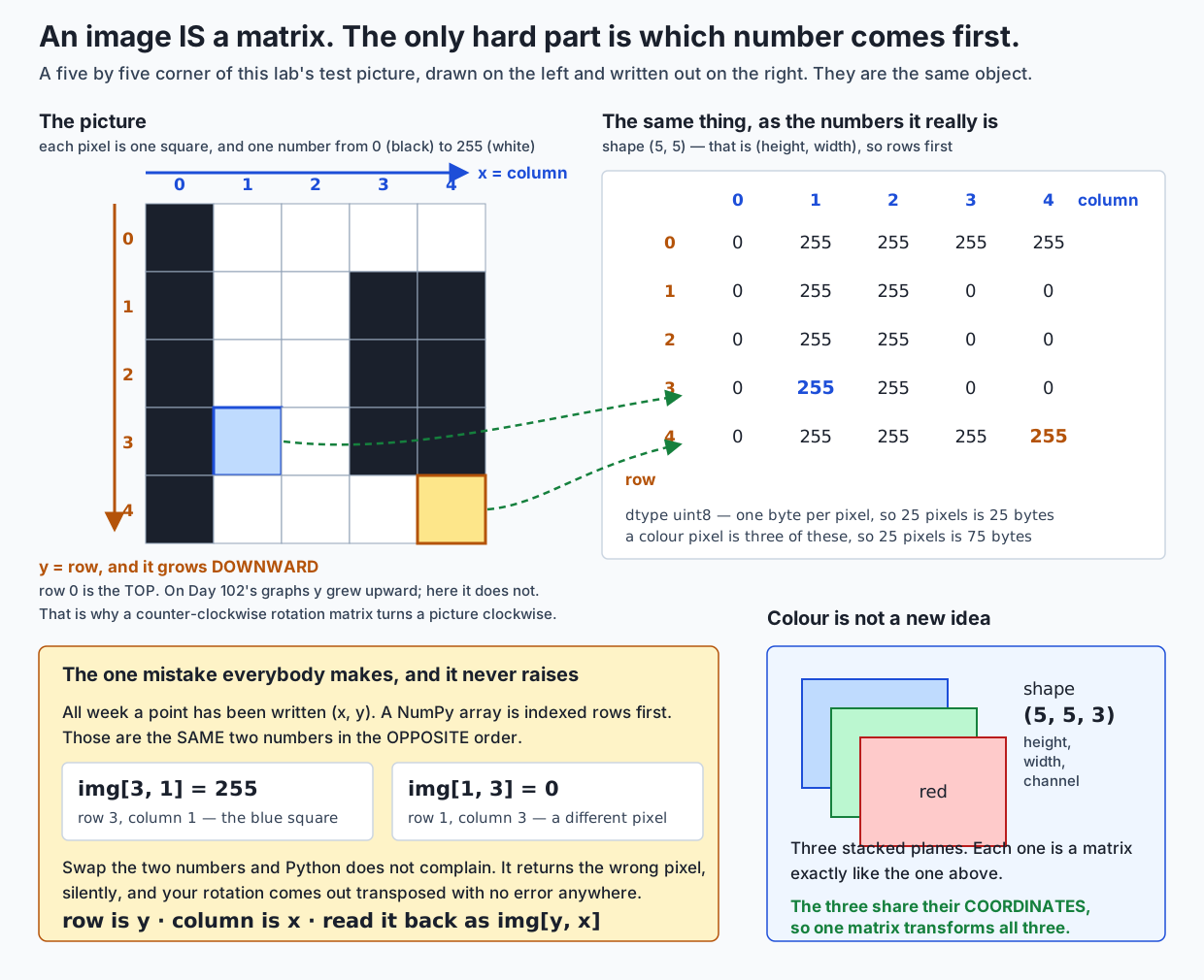
A greyscale image is a two-dimensional array of shape (height, width). A colour image is (height, width, 3) — three stacked planes, one each for red, green and blue.
Here is the test picture this lesson and its lab both use, generated in code rather than downloaded. It is a capital F on a nine-by-nine grid:
.######..
.##......
.##......
.##......
.####....
.##......
.##......
.##......
.##.....o
. is 0, # is 255, and o is a single grey pixel at 96 in the bottom-right corner. It is an F for one specific reason: an F is asymmetric under every operation in this lesson. A square survives a horizontal flip unchanged, so a broken flip applied to a square would pass its own test. An F survives nothing — flip it, rotate it, transpose it, and you can see at a glance which one happened.
Now the trap, and it is worth more attention than anything else in this section because it is the single most common source of confusion in the subject.
A NumPy array is indexed rows first. All week, a point has been written (x, y). Those are the same two numbers in the opposite order.
img.shape       = (9, 9)     <- (height, width) = (rows, columns)
img[4, 3] = 255   (row 4, column 3)
img[3, 4] = 0     (row 3, column 4)
Two different pixels. Swap the numbers and Python does not complain — there is no error, no warning, and no clue. It returns the wrong value, and your rotation comes out transposed, and you spend an hour reading the matrix arithmetic looking for a sign error that is not there.
The rule, and it is worth writing on something:
Row is y. Column is x. A point
(x, y)is read back asimg[y, x].
There is a second half to the convention. The origin is the top-left corner and y grows downward, because row 0 is the first row of memory and screens have always been drawn top row first. Day 102’s graphs had y growing upward, as graph paper does. Nothing about the matrices changes — but the picture is flipped relative to the graph paper, and the visible consequence is that Day 102’s counter-clockwise rotation matrix turns an image clockwise on screen.
That is not a sign error and you should not fix it. The lab asserts it:
  before                     after
    .######..                .........
    .##......                #########
    .##......                #########
    .##......                ....#...#
    .####....                ....#...#
    .##......                ........#
    .##......                ........#
    .##......                .........
    .##.....o                o........
The F turned clockwise, from the counter-clockwise matrix. And the corner mark went from row 8, column 8 to row 8, column 0 — bottom-right to bottom-left, which is what a clockwise quarter turn does to a bottom-right corner.
Colour adds no new mathematics at all, which is the point worth noticing. The three planes share their coordinates, and the transformation acts on coordinates, so the same matrix does all three.
Transforming coordinates, not pixels
Take the corner mark. It sits at row 8, column 8, so as a point it is (x, y) = (8, 8). Move it by (+2, −3):
  Move it by (+2, -3):  (10.0, 5.0)
  Nothing was done to any pixel VALUE. The coordinate moved.
That line is the whole conceptual content of the day. The grey level 96 is still 96. What changed is which slot in the grid it occupies.
So “rotate the image” decomposes into: work out, for each pixel, where its coordinate goes; then move the value there. And the second half of that sentence is where it all comes apart.
Forward mapping, and why it leaves holes
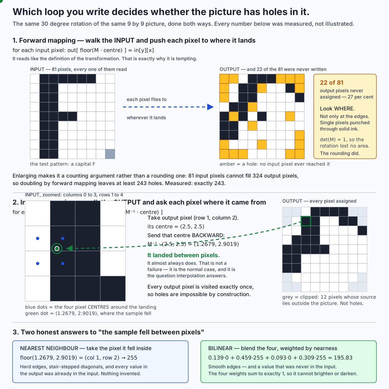
Forward mapping is the loop from the opening:
for each INPUT pixel:
    send its centre through the matrix
    take the output pixel that point falls in
    write the value there
It is the definition of the transformation, read aloud. And it fails, in three distinct ways depending on what the transformation does.
Rotating: holes. The measured result on the test picture, from a real run:
A 30 degree rotation about the centre
  forward mapping: 22 of 81 output pixels were never written (27.2%)
Notice what that number is not caused by. A rotation’s determinant is exactly 1 — Day 102’s signed area, unchanged — so the rotation cannot create extra room that needs filling. What happens instead is that the input pixels land on non-integer positions that round unevenly: some output pixels collect two input pixels, and their neighbours collect none. The area is conserved; the coverage is not.
Enlarging: holes, and now it is arithmetic rather than accident.
  Scale by 2. Input has 81 pixels; output has 324.
  At most 81 output pixels can ever be written, so at least
  243 MUST be holes. Measured: 243.
That is a counting argument. Eighty-one input pixels cannot fill three hundred and twenty-four output pixels however carefully you place them, and no amount of care in the loop changes it. Here is what three-quarters-missing actually looks like:
~~~~~~~~~~~~~~~~~~
~.~#~#~#~#~#~#~.~.
~~~~~~~~~~~~~~~~~~
~.~#~#~.~.~.~.~.~.
~~~~~~~~~~~~~~~~~~
~.~#~#~.~.~.~.~.~.
A regular lattice of gaps, which is the fingerprint of a forward-mapped enlargement.
Shrinking: no holes at all, and still wrong.
  Scale by a half into a 5 by 5 output: 0 holes.
  24 of the 25 output pixels were written more than
  once; the busiest received 4 input pixels.
  Example: output pixel (0, 0) was written by input pixels [(0, 0), (0, 1), (1, 0), (1, 1)].
Every output pixel got a value, so there is nothing obviously broken. But four input pixels landed on output pixel (0, 0) and overwrote each other, so which one survived was decided by the order of the loop rather than by anything about the picture. Change the iteration order and you get a different image. That is a worse failure than a hole, because it does not announce itself.
The tempting fix is to find the holes afterwards and fill each one from its neighbours. Resist it. That is a second pass over the image, more code, slower, and it still guesses. There is a fix that costs nothing.
Inverse mapping, which cannot leave holes
Turn the loop inside out:
for each OUTPUT pixel:
    take its centre
    send it BACKWARD through the inverse matrix
    take the value of the input pixel containing that point
Every output pixel is assigned. That is not a claim about the arithmetic being better — it is a property of iterating over the array you are filling. You visit each slot exactly once and you write to it exactly once, so “never written” is not a state that can occur.
This is why warp_nearest in the lab takes the transformation you can see and inverts it internally, and it is why Pillow’s API takes coefficients in the output-to-input direction. The inverse is not an implementation detail; it is the direction the algorithm runs in.
Two things follow, and the second one is a genuine cost.
The fill-valued pixels that remain are clipping, not holes. After the same thirty-degree rotation, twelve output pixels take the fill value. The lab does not assert that they are clipping; it proves it, by mapping every one of them back and checking that its source lies outside the input:
  fill-valued output pixels: 12
  of those, sourced from outside the input: 12
  All of them. Inverse mapping has no holes at all.
The corners of a rotated square do not fit inside a square. Something has to go in those pixels, and what goes there is a decision you make — a fill colour, a mirror of the edge, a wrap-around, or an output canvas large enough that the question does not arise. It is a decision, not an error.
The transformation must be invertible. Inverse mapping needs the inverse, so a transformation with determinant zero — one that flattens the picture onto a line — cannot be applied at all. The lab raises before touching a single pixel:
    determinant: 0.0
    warp_nearest raised SingularTransform
    message: determinant is 0.0: this transformation collapses the image and cannot be undone
That is the right time for the error. Day 102 established that numpy.linalg.LinAlgError is itself a ValueError; SingularTransform follows the same pattern, so an existing except ValueError keeps working.
The half-pixel, and the question Day 102 left open
Here is the detail that decides whether your implementation agrees with a real library or is subtly adrift.
Every pixel is a little square. Pixel (x, y) covers the region from (x, y) to (x + 1, y + 1). Its centre — the point that represents it — is at (x + 0.5, y + 0.5), not at its corner.
So the transformation is evaluated at the centre:
source_x = a·(out_x + 0.5) + b·(out_y + 0.5) + c
source_y = d·(out_x + 0.5) + e·(out_y + 0.5) + f
and then you take floor of each, because you want the input pixel whose square contains that point.
Day 102 confirmed by experiment that Pillow’s coefficients run output-to-input, and it explicitly deferred one thing to today: a half-pixel sampling offset that appeared to make a shear coefficient act on row 0, which the mathematics says is impossible because the shear term is multiplied by y and row 0 has y = 0.
It is settled, and the answer is that row 0 is not at y = 0. Its output pixels are sampled at their centres, which are at y = 0.5. So a shear coefficient of 2.0 contributes 2.0 × 0.5 = 1.0 — one whole pixel — even in the top row.
The lab measures it three ways rather than asserting it. First, the two candidate rules are separated by a single experiment. Take the row 0, 10, 20, …, 70 and halve it with a = 2:
    input             [0, 10, 20, 30, 40, 50, 60, 70]
    Pillow observed   [10, 30, 50, 70, 32, 32, 32, 32]
    rule A predicts   [10, 30, 50, 70, 32, 32, 32, 32]
    rule B predicts   [0, 20, 40, 60, 32, 32, 32, 32]

    matches rule A?  True
    matches rule B?  False
Rule A is floor(a·(x + 0.5) + …) — pixel centres. Rule B is floor(a·x + … + 0.5) — integer corners with rounding. The two agree on every integer translation, which is exactly why Day 102 could not tell them apart from a translation experiment and said so instead of guessing.
Second, the shear itself:
    a vertical line at x = 4, with b = 2:
      row 0: line now at x = 3    shift predicted by rule A: 1
      row 1: line now at x = 1    shift predicted by rule A: 3
Row 0 moved. Predicted exactly.
Third, in the from-scratch implementation, where the rule can be varied and the consequence measured:
    x_source = floor((x + 0.5) - k * 0.5)
    k = 0.5:  floor(x +0.25) = x +0   ->  the content moves right by 0
    k = 1.0:  floor(x +0.00) = x +0   ->  the content moves right by 0
    k = 2.0:  floor(x -0.50) = x -1   ->  the content moves right by 1
Leave the half out and every result is displaced by half of whatever the transformation does — which looks like a mysterious blur rather than like an offset, and is much harder to diagnose than a clean error.
Homogeneous coordinates, and why translation needed them
Day 102 proved a linear map cannot move the origin. Here it is again, measured, because the proof is one line:
    rotation(1.1)    sends the origin to (0.0, 0.0)
    scaling(4, 0.2)  sends the origin to (0.0, 0.0)
    shear_x(9)       sends the origin to (0.0, 0.0)
Every two-by-two matrix does that, by construction: the result is the columns weighted by the input coordinates, and weighting anything by zero and zero gives zero. Translation by (3, 0) sends the origin to (3, 0). Therefore translation is not linear, and no two-by-two matrix performs it.
The fix is to write the point (x, y) as the triple (x, y, 1). Now a three-by-three matrix can add a constant, because the constant is multiplied by that 1:
      [ 1  0  tx ] [ x ]   [ x + tx ]
      [ 0  1  ty ] [ y ] = [ y + ty ]
      [ 0  0   1 ] [ 1 ]   [   1    ]
The third coordinate is not a z axis and the picture has not become three-dimensional. It is a bookkeeping device: one extra slot whose only job is to give the translation something to multiply.
Two immediate consequences.
A translation’s determinant is exactly 1 — it moves the picture without changing its area — and its inverse is the opposite translation. Both checkable by eye, both asserted in the lab.
And a flip stops being awkward. A bare reflection sends x to −x, which puts the whole picture off the left edge. What you actually want is a mirror about the image’s own centre line, sending x to width − x — which is a reflection followed by a translation, and is therefore one matrix rather than two steps:
      [ -1.0    0.0    9.0 ]
      [  0.0    1.0    0.0 ]
      [  0.0    0.0    1.0 ]
Applied to the nine-wide test picture, that is exactly numpy.fliplr. Not approximately — the lab asserts equality, because nearest-neighbour produces whole pixel values and there is nothing to round.
Composing, and why it is both cheaper and more accurate
Rotating about the image’s centre rather than its top-left corner is three steps: move the centre to the origin, rotate, move it back. It is also one matrix, and this is where homogeneous coordinates earn their place — without them the middle step is a matrix and the two outer steps are not, so they cannot be multiplied together at all.
combined = T(+c) · R · T(-c)Read the product right to left: the rightmost matrix acts first. That is the Day 101 convention and it has not changed.
Now the measurement that matters. Take three operations — rotate thirty degrees, shear, scale — and apply them two ways.
three resampling passes vs one: 36 of 324 pixels differ (11.1%)Eleven per cent of the picture is different, and the composed version is the correct one. Each intermediate resample in the three-pass version quantised the picture to whole pixels and threw the remainder away, and the next pass had no way to know what had been lost.
The same point, in its starkest form. A full turn — 360 degrees — should return the original image:
  rotation(2*pi) applied once, differing pixels: 0
  twelve separate 30 degree rotations, differing pixels: 16
Both routes are a full turn. One is exact and one loses sixteen of eighty-one pixels. The difference is not the angle; it is how many times the image was resampled. And composing those same twelve rotations into one matrix and applying it once:
  the same twelve rotations COMPOSED into one matrix and applied
  once, differing pixels: 0
Exact again. The matrices cost nine multiplications each to combine; the pixels cost a full pass over the image. Composing is more accurate and cheaper.
One more note on that zero, because “exact” deserves scrutiny. The full-turn matrix is not exactly the identity — sin(2π) comes out as about −2.45e−16, not 0. The residual displacement is around a quadrillionth of a pixel, and nearest-neighbour rounds to a whole pixel, so an error fifteen orders of magnitude below the rounding step cannot change the answer. The float error is real and it is absorbed. That will not be true of every angle, which is why the lab also provides an exact-integer quarter-turn matrix for the cases where the answer is meant to be checkable.
Interpolation: the sample landed between pixels
The inverse-mapped position almost never lands on a pixel exactly. It is not supposed to. Take output pixel row 1, column 2 under the thirty-degree rotation:
its centre = (2.5, 2.5)
M⁻¹ · (2.5, 2.5) = (1.2679, 2.9019)
That is between pixels. Two honest answers, and the choice between them is the whole of interpolation at this level.
Nearest neighbour takes the pixel the point fell inside: floor(1.2679, 2.9019) is column 1, row 2, whose value is 255. Hard edges, stair-stepped diagonals, and — the property that matters more than it sounds — every value in the output was already in the input. Nothing is invented, so nearest-neighbour is the correct choice for label masks, segmentation maps and any image whose pixel values are categories rather than quantities. Averaging two class labels gives you a class that does not exist.
Bilinear blends the four pixels surrounding the point, weighted by nearness:
0.139·0 + 0.459·255 + 0.093·0 + 0.309·255 = 195.83The four weights sum to exactly 1, which is why bilinear cannot brighten or darken an image overall. The result, 195.83, is a value that was never in the input — which is the point, and also the cost.
The half-pixel bookkeeping is the fiddly part of implementing it. A pixel’s value lives at its centre, (i + 0.5, j + 0.5), so to interpolate between centres you subtract the half back off before splitting into whole and fractional parts. Getting this wrong shifts the whole image by half a pixel, which reads as a mysterious softness rather than as an offset.
The visible difference is easy to state: nearest-neighbour preserves values and produces jagged edges; bilinear produces smooth edges and produces values that were not there. Which is a defect depends entirely on what your pixels mean.
Ours against Pillow: where it agrees, and where it does not
This is the day’s strongest artifact, and it is only worth anything because the from-scratch code deliberately does not use NumPy for its matrix arithmetic. The matrices are plain nested lists and the multiplication is written out by hand. NumPy holds the pixels, because a grid of bytes is what NumPy is for; the mathematics is ours. If rotation had returned a NumPy array built by a NumPy helper, then agreeing with a library that sits on the same numerical machinery would prove very little.
First, the convention, re-verified rather than recalled. Pillow’s Image.transform(size, AFFINE, (a, b, c, d, e, f)) means
input_x  =  a · output_x  +  b · output_y  +  c
input_y  =  d · output_x  +  e · output_y  +  f
— output to input, the inverse of the effect you see:
    a single bright pixel at input x = 3
    coefficients (1, 0, 1, 0, 1, 0), so c = +1
    the bright pixel comes out at x = 2
    the content moved LEFT by 1 when c said +1.
So the coefficients are read off the inverse of the matrix you mean, and to_pillow_coefficients(translation(1, 0)) is (1.0, 0.0, -1.0, 0.0, 1.0, 0.0). Note the minus. Forgetting to invert is the most common way to get a Pillow transform backwards, and it does not raise — it just moves the picture the wrong way.
Now the comparison. Five hundred random rotate-scale-shear-translate combinations plus ten deliberate edge cases, each handed to both implementations as the identical six numbers:
    transformations compared:            510
    transformations matching EXACTLY:    510
    worst case, pixels differing:        0
    stated tolerance for this comparison: 0 (exact equality)
Every pixel of every one of them. Twenty-odd lines of arithmetic and a library maintained since the 1990s producing byte-for-byte the same array.
It would be easy to stop there. It would also be misleading, and the honest half is more useful than the headline. Sweep every whole-degree rotation — 360 transformations chosen to be nothing like random — and:
    rotations compared:                 360
    identical, pixel for pixel:         352
    disagreeing in at least one pixel:  8
    worst case, pixels differing:       2 of 81
    the angles: [30, 60, 120, 150, 210, 240, 300, 330]
Eight angles, never more than two pixels of eighty-one. And every single disagreeing sample landed within 2.220e-15 of a pixel boundary. Here is the smallest failing case in full:
    output pixel (row 4, column 3): ours 255, Pillow 0
      our source y = 4.999999999999999
      floor of that = 4; Pillow took row 5
The exact answer is 5. The sample sits precisely on the boundary between two pixels, and which one you get is decided by the order the floating-point additions happen in — Pillow’s C loop walks along each output row accumulating the source coordinate step by step, while this implementation evaluates the whole expression per pixel. Same formula, different rounding in the last bit. Neither is wrong.
Look at which angles failed: 30, 60, 120, 150, 210, 240, 300, 330. Every one is a “nice” angle whose sine or cosine is exactly a half or exactly half the square root of three — which is what puts samples exactly on boundaries. The angles nobody would think to test, 37 degrees and 113 degrees, all agreed. Round numbers are where floating-point ties live, which is the opposite of most people’s intuition about which test cases are safe.
The practical rule that falls out: if you need bit-identical output across libraries, do not rely on ties breaking the same way. Either keep your samples away from boundaries, or accept a one-pixel tolerance and say so in writing.
The bilinear comparison splits just as cleanly, and it is stated here rather than smoothed over:
    transformation                all 4 inside    anywhere
    translate (0.25, 0.25)               0.938      63.750
    rotate 30 about the centre           1.000     118.346
    scale 1.5 about the centre           1.000       1.000
    shear x by 0.4                       1.000      32.000
Wherever all four contributing pixels are inside the image, the two agree to within one grey level — which is exactly the rounding of a float average back into a byte and cannot be improved on. Wherever a contributor lies outside the image, they diverge by up to 118 levels, because they extrapolate differently: this implementation averages the fill value in, and Pillow does not. That border behaviour was measured, not assumed, and it was not chased further, because naming the boundary of what agrees is more useful than widening a tolerance until a test goes green.
An everyday analogy
You are copying a mosaic from one wall onto another, and the new wall is set at an angle to the old one.
Forward mapping is working from the old wall. You take the first tile, work out where it belongs on the new wall, and cement it there. Then the next. It feels like the obvious method — you are copying the mosaic, so you work through the mosaic. But when you step back at the end, the new wall has gaps in it. Not just at the edges where the angled copy ran off the wall, but scattered through the middle, because the old grid and the new grid do not line up and two old tiles occasionally want the same new slot while the slot beside it gets nobody. If you are copying onto a bigger wall it is worse and it is obvious in advance: a thousand old tiles cannot fill four thousand new slots.
Inverse mapping is working from the new wall. You stand at the first empty slot, look back through the angle at the old wall, and ask: what was at this spot? Then you fill the slot with that. Then the next slot. When you have been to every slot, the wall is complete — not because you were careful, but because you went to every slot. That is the whole argument, and it is why every library does it this way.
The analogy carries the rest of the day too, which is why it is worth setting up properly.
When you look back through the angle, the spot you are looking at almost never sits neatly on one old tile. It usually falls near a corner where four tiles meet. Nearest neighbour is deciding “I am mostly standing over that tile, I will copy that colour.” Fast, and every colour on the new wall was a colour on the old wall. Bilinear is mixing paint from all four in proportion to how close you are standing to each — smoother, and it produces colours that were never in the original mosaic.
Clipping is the slots near the edge of the new wall where looking back through the angle points you off the old wall entirely. There was nothing there. You have to decide what to put in those slots, and that decision is yours.
Composing is the reason you do not copy the mosaic onto an intermediate wall first. Every copy loses a little — each time you snap a mixed colour onto a discrete tile, the remainder is gone. Work out the total angle first, then make one copy.
Two places the analogy honestly breaks, and it is worth naming them rather than letting them mislead:
Real tiles cannot be subdivided, and real paint mixing is not the same as averaging light — mixing red and green paint gives you a muddy brown, whereas averaging red and green pixel values gives you something closer to yellow. The mathematics of bilinear interpolation is averaging light, not mixing pigment.
And the mosaic has no equivalent of the floating-point tie. In the real world, standing exactly on the line between two tiles is a situation you resolve by looking; in floating point it is resolved by the order of your additions, which is why the eight nice angles disagreed.
Examples in practice
Displaying a photograph the right way up. Cameras store the sensor readout and record the orientation separately, in EXIF metadata. Your viewer reads that tag and applies one of eight transformations — the four rotations and their mirrors — before drawing. All eight are affine, all eight are exact (they are quarter turns and flips, so every pixel lands on a pixel), and none of them needs interpolation at all. This is the case where a transformation is free of cost.
Deskewing a scanned document before text recognition. A page fed slightly crooked comes out at maybe two degrees off. Text recognition degrades sharply with skew, so the pipeline estimates the angle and rotates. Two degrees is not a nice angle, so interpolation matters and bilinear is the usual choice — text is a quantity, not a category, and smooth edges recognise better than jagged ones.
Registering two medical scans. The same patient, two dates, two slightly different positions in the machine. To compare them you must transform one into the other’s frame. Here the transformation is the measurement, and getting it wrong invents a change that is not there. Note that this is also a case where a flip is not a legitimate operation, for reasons the AI thread returns to.
Augmenting a training set. Every image, every epoch, rotated and flipped and shifted by a random amount. This is the highest-volume use of the operation by a very wide margin, and it is where composing matters most: a pipeline that resamples three times per image is doing three times the work to produce a worse result.
Building a texture atlas or a sprite sheet in a game. Every frame, thousands of quads are transformed by affine matrices before being drawn. The graphics hardware does this natively — the matrix goes to the GPU once and the transformation of every vertex happens in parallel — and the reason the API asks for a matrix rather than a rotation angle is exactly today’s composition argument: one matrix can carry an entire chain of operations.
Implications: security, privacy, performance, scalability, and cost
Performance. Inverse mapping costs one pass over the output, which means the cost is proportional to the output size rather than the input size. Downscaling is therefore cheap and upscaling is expensive, which is the opposite of what people often assume. The from-scratch implementation in the lab is a plain Python double loop, which is fine for a nine-by-nine picture and unusable for a real photograph — Pillow’s version is C, and the same operation on a twelve-megapixel image is milliseconds rather than minutes. That gap is Day 104’s argument about vectorised code, in its most extreme form.
Precision cost, which is the one people miss. Every resampling pass quantises the picture and discards the remainder. The measurements are in this lesson: eleven per cent of pixels different between three passes and one, and sixteen of eighty-one lost by twelve rotations that add up to nothing. If your pipeline has more than one geometric step, compose them.
Memory. A greyscale image is one byte per pixel; a colour image is three. A twelve-megapixel colour photograph is thirty-six megabytes as a raw array, and an intermediate copy per transformation step is another thirty-six each. This is a second, purely practical reason to compose: one matrix means one intermediate, not four.
Scalability. Augmentation happens per image per epoch, so its cost multiplies by dataset size and by training length. A pipeline that is twenty per cent slower than it needs to be is twenty per cent of your entire training budget, and it is the kind of waste that hides easily because nobody profiles the data loader.
Security. The lab needs the network exactly once, to install three packages, and generates its own test image rather than downloading one — which is a security decision as much as a pedagogical one. Working with images from elsewhere carries two real hazards worth naming. Image decoders are complex C parsers running over bytes you did not write, and they have a long history of memory-safety bugs; keep your library current and do not decode untrusted images in a process holding anything valuable. And decompression bombs — small files declaring enormous canvases — are a real denial-of-service vector. Pillow defends against this by default with a pixel-count limit, and Image.MAX_IMAGE_PIXELS = None is a widely copy-pasted line that removes a genuine protection.
Privacy. Geometric transformation does not anonymise anything. Rotating or cropping a photograph removes none of its metadata and none of its identifying content, and a downscaled face is often still recognisable, both to a person and to a model. If you need to remove information, remove it deliberately — strip the EXIF, redact the region — and do not assume a resize did it for you.
Cost. All of the tooling here is free. The costs are compute time and, if you get the precision argument wrong, model accuracy — which is a slower and more expensive thing to discover.
Alternatives: free, open source, and commercial
The honesty statement first, because it decides how to read everything below. Only NumPy 2.5.2 and Pillow 12.3.0 were actually run for this lesson, on Python 3.14.0 on macOS 26.5.2. Every output block above came from a real run on the authoring machine. The other tools in this section are described from their published documentation and their behaviour is not reproduced here, because they are not installed.
Your own NumPy implementation — free, and the one to write first.
When to choose it: when you are learning, when you need behaviour a library will not give you, or when you need to know exactly what your pipeline is doing to your data. Also when the operation is exact — a quarter turn or a flip — where numpy.rot90 and numpy.fliplr are a single call and cannot be beaten.
How to use it: build the three-by-three matrix, invert it, loop the output, sample at pixel centres, floor. That is the whole thing.
Concrete example, run here: the twelve functions in the lab’s warp.py come to a few dozen lines and reproduce Pillow byte-for-byte on 510 of 510 test transformations.
Free vs paid: free. NumPy is BSD 3-Clause.
The honest limitation: a Python double loop over a real photograph is unusably slow. You can vectorise it with numpy.meshgrid and fancy indexing — which is a genuinely good exercise and the natural sequel to Day 104 — but at that point you are reimplementing a library.
Pillow — free, and the one that was run here.
When to choose it: general-purpose image work in Python where you are not already in a computer-vision or deep-learning stack. It reads and writes essentially every format, it is a small dependency, and it is the library most other Python image code expects.
How to use it:
from PIL import Image
out = image.transform(
    (width, height), Image.Transform.AFFINE, coefficients,
    resample=Image.Resampling.NEAREST, fillcolor=32,
)
with coefficients read off the inverse of the matrix you mean.
Concrete example, run here: the entire section-six comparison, including the measurement that settled Pillow’s sampling rule and the eight rotations where it and this implementation break a tie differently.
Free vs paid: free. MIT-CMU licence, no account, no key.
Note: Image.rotate and Image.resize are convenience wrappers over the same machinery, and Image.rotate(angle, expand=True) handles the “corners fall outside the frame” problem for you by sizing the output to fit.
OpenCV (cv2) — free, open source, and NOT installed or run here.
What it adds: speed and breadth. cv2.warpAffine and cv2.warpPerspective are heavily optimised, it offers interpolation rules beyond nearest and bilinear — bicubic, Lanczos, and an area-averaging mode that is the right choice for large downscales — and it provides cv2.getAffineTransform and cv2.getPerspectiveTransform, which solve for the matrix given corresponding points. That last one is the answer to “I know where three corners should end up” and it is genuinely hard to write yourself.
When to choose it: real-time work, video, or anything where you also need feature detection, camera calibration or lens-distortion correction. It is the only tool in this list that handles projective transformations and lens distortion, both of which this lesson said affine cannot do.
Free vs paid: free, Apache 2.0.
No output is reproduced here. It is not installed on the authoring machine and this lesson will not quote behaviour it has not observed.
scikit-image — free, open source, and NOT installed or run here.
What it adds: a clean, explicit model of transformations as objects. skimage.transform.AffineTransform and SimilarityTransform are constructed from named parameters — rotation, scale, shear, translation — rather than from six raw numbers, they compose with +, and estimate fits a transform to point correspondences including a RANSAC variant that tolerates bad matches. It fits naturally alongside the rest of the scientific Python stack.
When to choose it: scientific and analytical image work, especially registration, where being able to say what the transformation means matters more than raw throughput.
Free vs paid: free, BSD 3-Clause.
No output is reproduced here.
torchvision transforms — free, open source, and NOT installed or run here.
What it adds: augmentation as a first-class part of a training pipeline. torchvision.transforms.v2 provides RandomAffine, RandomRotation, RandomHorizontalFlip and the rest, composable into a pipeline, operating on tensors, running on the GPU, and — the part that matters and that the others do not do — transforming bounding boxes and segmentation masks alongside the image, so your labels stay correct when the picture moves.
When to choose it: you are training a model in PyTorch. That is essentially the whole answer.
Free vs paid: free, BSD 3-Clause.
No output is reproduced here.
Commercial image editors. Photoshop, Affinity Photo and their peers do all of this behind a menu, with better default resampling than any of the above, and are the right tool when a human is judging the result. They are irrelevant to a training pipeline and none is required for anything in this course.
Comparison with related concepts
| Concept | What it does to coordinates | What it does to values | Reversible? |
|---|---|---|---|
| Affine transformation (today) | moves them by a 3×3 matrix; straight lines stay straight, parallels stay parallel | nothing, except through the interpolation rule | yes, if the determinant is not 0 — but resampling loses information each pass |
| Projective transformation | moves them by a 3×3 matrix whose bottom row is not (0, 0, 1), then divides by the third coordinate; straight lines stay straight, parallels do not | nothing directly | yes, if invertible |
| Lens distortion correction | moves them by a non-linear function of the distance from the optical centre; straight lines bend | nothing directly | approximately, and not by a matrix |
| Convolution | leaves them alone | replaces each value with a weighted sum of its neighbours | generally no |
| Colour transform (greyscale, contrast) | leaves them alone | maps each value through a function | sometimes |
The row worth staring at is the last two versus the first. Convolution and transformation are constantly confused because both involve a small matrix and an image, and they have nothing in common: one is geometry and the other is filtering.
A second comparison, since it decides a real choice:
| Nearest neighbour | Bilinear | |
|---|---|---|
| Output values | only values already in the input | new values, blended |
| Edges | hard, stair-stepped | smooth |
| Cost | one lookup | four lookups and three blends |
| Right for | label masks, segmentation, palettes, exact quarter turns | photographs, any continuous quantity |
| Wrong for | photographs at odd angles, where it looks jagged | anything whose values are categories |
| Measured here | matches Pillow on 510 of 510 cases, 0 pixels differing | matches Pillow within 1 grey level away from the border |
When to use it — and when not to
Use an affine transformation when straight lines should stay straight and parallel lines should stay parallel — rotating, scaling, shearing, flipping, translating, or any composition of those. That covers almost everything people mean by “transform an image”.
Use nearest neighbour when your pixel values are categories rather than quantities: segmentation masks, label maps, indexed-palette images. Blending class 3 and class 7 into class 5 is a silent data-corruption bug that will not show up until your metrics do.
Use bilinear when your pixel values are quantities and the transformation is not an exact quarter turn. Photographs, depth maps, intensity images.
Use an exact quarter turn or flip when you can, and use numpy.rot90 or numpy.fliplr to do it. They are exact, they need no interpolation, they are a single call, and they are far faster than anything general.
Do not use an affine transformation when you need perspective — a projective transform is the tool, and its matrix is the same size with a different bottom row and one division. Do not use it for lens distortion, which no matrix expresses. Do not use it for warping one shape into another, which needs a displacement field.
Do not resample twice when once will do. If there is a rotation and a scale and a translation, multiply the matrices and make one pass. The measurements are above; this is the single most common avoidable quality loss in an image pipeline.
Do not assume ties break the same way across libraries. Eight of 360 whole-degree rotations differ between this lesson’s implementation and Pillow’s. If you have a test asserting pixel-exact agreement with a library, either pick angles away from boundaries or state a one-pixel tolerance.
Do not upscale expecting detail. Enlarging gives you more pixels and not one bit more information. The lab measures this: doubling the test picture produced exactly the same three distinct pixel values it started with.
The AI thread
Augmentation for training is exactly this lesson, run at volume. Random rotations, flips, shears and shifts applied to every training image every epoch, so that the model learns that a cat tilted eight degrees is still a cat, rather than learning that cats are upright. It is one of the cheapest regularisers available and it is nothing but the arithmetic above.
Which makes the question of which augmentations are legitimate a real one, and it is worth one honest paragraph because it is easy to get wrong. A horizontal flip is a fine augmentation for photographs of animals and objects, because a mirrored cat is a perfectly plausible cat and your model will meet plenty of them. It is not legitimate for text, because mirrored text is not text and you have just taught your model that a letter and its mirror image mean the same thing — which will cost you exactly on the letters where it matters, like b and d. And it is not legitimate for many medical scans, because human anatomy is not left-right symmetric: the heart is on one side, the liver is on the other, and situs inversus — the condition where they are reversed — is a real and clinically significant finding. Flipping chest X-rays as an augmentation teaches a model that a rare, important condition is normal. The rule underneath all three cases is the same: an augmentation is legitimate exactly when the transformed image is one that could genuinely occur in your data with the same label. That is a question about your domain, not about your library, and no default setting can answer it for you.
One more connection, and it is a distinction rather than a link. Convolution — the operation the deep-learning course reaches later, and the thing the “convolutional” in CNN refers to — also acts on an image matrix, and people conflate it with transformation constantly. They are different operations on the same object. A transformation moves coordinates and leaves values untouched. A convolution leaves coordinates untouched and replaces each value with a weighted combination of its neighbours. Today’s matrix says where things go; a convolution kernel says how neighbouring values combine. Knowing that an image is a matrix is what makes both of them make sense, and this is the day you learned it.
Knowledge check
Eight questions in quiz.yml, including one on why every real implementation uses inverse mapping and one on why translation needs homogeneous coordinates.
Hands-on exercise
Work through the lab: labs/sections/math-statistics-and-data/day-105-transforming-images-with-matrices/.
Read starter/00_brief.md, then write the twelve functions in starter/warp.py and the twenty-six predictions in starter/answers.py.
cd labs/sections/math-statistics-and-data/day-105-transforming-images-with-matrices
python3 -m venv .venv
.venv/bin/pip install -r requirements/requirements.txt
.venv/bin/pytest starter -q
The spine of the work, in order:
- Generate the test pattern and assert its known pixel values. Nothing is downloaded.
- Implement forward mapping and assert the holes exist — count them. Do not patch them.
- Implement inverse mapping with nearest-neighbour, and assert that a quarter turn puts known pixels in exactly the right places.
- Implement scale, shear and flip the same way, each checked against an independent NumPy answer.
- Compose two transformations into one matrix and assert it equals applying them in sequence.
- Add homogeneous coordinates and assert that translation works as a matrix multiply.
- Compare your implementation against Pillow’s
Image.transformon the identical six coefficients. - Assert that a 360-degree rotation returns the original image — and find out for yourself which route is exact and which is not.
Expected output
An untouched checkout:
1 passed, 53 skippedA finished one:
54 passedThe full harness, from a real run on the authoring machine:
Day 105 — Rotate It Yourself

1. The tools and the versions this lab was written against
  python   3.14.0
  numpy    2.5.2
  pillow   12.3.0
  pytest   9.1.1
  platform macOS-26.5.2-arm64-arm-64bit-Mach-O
and its last line:
79 checks, 0 failure(s).The comparison the day is built around:
    transformations compared:            510
    transformations matching EXACTLY:    510
    worst case, pixels differing:        0
and the half that makes it honest:
    rotations compared:                 360
    identical, pixel for pixel:         352
    disagreeing in at least one pixel:  8
    worst case, pixels differing:       2 of 81
    the angles: [30, 60, 120, 150, 210, 240, 300, 330]
Validate your work
.venv/bin/pytest examples -qprints64 passed..venv/bin/pytest starter -qprints54 passedwhen you are done.- Each of the six reference scripts exits 0 and ends with
every assertion held. bash tests/run_tests.sh; echo "exit=$?"prints79 checks, 0 failure(s).andexit=0. Check the exit status directly, not through a pipe.- Your output matches
expected-output/, allowing for the machine-dependent fields named inFIELDS.md.
Troubleshooting
Everything is half a pixel out. You left SAMPLE_OFFSET out of the sampling, or added it to one coordinate and not the other. Confirm with the downscale test: halving must equal img[1::2, 1::2] — note the 1, not 0. Output pixel 0 has its centre at 0.5, which doubles to 1.0.
The Pillow comparison disagrees on a scattering of pixels. You used int() or round() instead of math.floor(). int(-0.3) is 0 and math.floor(-0.3) is −1, so int duplicates a row and a column at the top-left edge; round is a different rule that disagrees on half of all inputs.
The picture moves the wrong way through Pillow. You passed your matrix instead of its inverse. to_pillow_coefficients(translation(1, 0)) must be (1.0, 0.0, -1.0, 0.0, 1.0, 0.0) — the c is negative.
pytest starter reports failures rather than skips. Either you deleted a raise NotImplementedError without writing the body — the skip mechanism catches that exception — or you ran pytest from inside starter/ instead of from the lab directory.
Your eight disagreeing angles differ from the lab’s. That may not be your fault, and expected-output/FIELDS.md explains why. Which side of an exact tie you land on depends on the build. The claim that must hold is the check beside it: every disagreeing sample must land within 1e-9 of a pixel boundary. If that also fails, look at floor versus round.
Common mistakes
Swapping row and column. img[y, x], always. It never raises; it just returns the wrong pixel, and your rotation comes out transposed.
Patching the holes instead of inverting the loop. The holes are the argument, not the problem. Inverting the loop removes them entirely and costs nothing.
Sampling at the pixel corner instead of its centre. Half a pixel of error looks like softness rather than like an offset, which makes it much harder to find.
Resampling repeatedly instead of composing. Twelve thirty-degree rotations lose sixteen of eighty-one pixels; the same full turn as one matrix loses none.
Expecting a counter-clockwise matrix to look counter-clockwise. On an image, y grows downward, so it turns clockwise. That is the coordinate system, not a sign error.
Reflecting about the origin instead of the centre line. x → −x sends the picture off the left edge. You want x → width − x, which is a reflection and a translation, in one matrix.
Using bilinear on a segmentation mask. Averaging class 3 and class 7 gives class 5, which is a class that was never there.
Practice assignment
Write a function rotate_without_clipping(image, degrees) that rotates an image about its centre and returns an output large enough that nothing is clipped.
The work is in the sizing, not the rotation. Transform the four corners of the input, find the bounding box of the results, size the output to that box, and add the translation that shifts the picture into it — all composed into one matrix, applied in one pass.
Then check yourself two ways. Assert that no output pixel takes the fill value where a source pixel exists — that is, that the ink count is preserved. And compare against Image.rotate(degrees, expand=True), which does exactly this. Report the agreement honestly: state the number of differing pixels, and if there are any, check whether they are at boundary ties before assuming you have a bug.
Extension challenge
Vectorise the transformation, and measure what it buys you.
The lab’s implementation is a Python double loop, which is correct and unusably slow on anything larger than a test pattern. Rewrite it with the tools from Day 104: build the output coordinate grid with numpy.meshgrid, apply the inverse matrix to all coordinates at once as a single array operation, and gather the source pixels with fancy indexing.
Three things to get right, and each of them is a real trap:
- The half-pixel offset applies to the whole grid, before the matrix.
- Out-of-range indices must be masked before indexing, not clipped, or the edges will silently wrap or clamp instead of taking the fill value.
numpy.floorreturns floats; you must cast to an integer type before using the result as an index.
Assert that your vectorised version produces output identical to the loop version on the test pattern — exact equality, since nearest-neighbour produces whole values. Then time both on a larger generated image, say 512 by 512, and report the speedup you actually measured on your machine, with the size and the number of repetitions stated. Do not quote a figure from anywhere else.
If you want to go further: implement a projective transform. Allow the bottom row of the matrix to be something other than (0, 0, 1), divide the first two output coordinates by the third, and watch parallel lines converge. That is the perspective transform this lesson said affine cannot do — and it is about five extra lines.
Quiz
Q1. You rotate an image by walking every input pixel, working out where the matrix sends it, and writing the value there. The result has single pixels missing from the middle of solid areas. Why?
- The rotation matrix has a sign error, so some pixels are sent outside the output
- Rotation does not preserve area, so the output is larger than the input can fill
- Floating-point error accumulates across the loop and eventually skips a pixel
- Nothing guarantees that every output pixel gets visited, because the loop runs over the input rather than over the output
Show answer
Answer: D. Nothing guarantees that every output pixel gets visited, because the loop runs over the input rather than over the output
The holes are a property of which array the loop iterates over, not of the arithmetic inside it. Walking the input means you visit every input pixel exactly once — but you have no control over which output pixels get written, and the rounded landing positions collide unevenly: some output pixels collect two input pixels while their neighbours collect none. On the 9 by 9 test picture a 30 degree rotation leaves 22 of 81 output pixels unwritten, including pixels punched through the middle of the glyph. The second option gets the geometry exactly backwards and is worth ruling out carefully: a rotation's determinant is exactly 1, so it preserves area precisely — which is why the holes cannot be blamed on the output being too big. The first option describes a real and common bug, but a sign error gives you a picture rotated the wrong way, not a picture with speckle in it. The third misunderstands the scale of floating-point error, which is around 1e-16 and never reaches a rounding boundary. The fix is not to patch the holes afterwards — that is a second pass that guesses — but to turn the loop inside out.
Q2. Why does every real image library use inverse mapping — walking the output and looking backward — rather than forward mapping?
- It is faster, because the inverse matrix is cheaper to compute than the forward one
- It is more numerically accurate, because the inverse matrix has smaller entries
- It visits every output pixel exactly once, so unassigned pixels are impossible by construction
- It is the only direction in which interpolation is defined
Show answer
Answer: C. It visits every output pixel exactly once, so unassigned pixels are impossible by construction
The guarantee is structural rather than numerical. If your loop runs over the output array, then by the time the loop ends you have been to every slot and written to every slot, so "never assigned" is not a state that can occur. That is not a claim about the arithmetic being better — it is a claim about which array you iterate. The first option is wrong twice over: inverting a 3 by 3 affine matrix is done once for the whole image and costs nothing either way, and inverse mapping's cost is proportional to the OUTPUT size, so upscaling is actually more expensive. The second is not a real property; the inverse of a rotation is another rotation with entries of exactly the same size. The fourth is tempting but false — you could interpolate in a forward-mapped scheme too, by splatting each input pixel across several output pixels with weights; it is just far more work and still does not guarantee coverage. One consequence worth carrying: because inverse mapping needs the inverse, a transformation with determinant 0 cannot be applied at all, and the error arrives before any pixel is touched.
Q3. Why does translation require homogeneous coordinates — a third coordinate fixed at 1 — when rotation, scaling and shear do not?
- Because translation moves the origin, and Day 102 proved that no linear map can do that
- Because translation changes the image size, and only a 3 by 3 matrix can encode a size change
- Because translation is the only transformation that needs floating-point coefficients
- Because a 2 by 2 matrix cannot represent negative offsets
Show answer
Answer: A. Because translation moves the origin, and Day 102 proved that no linear map can do that
Every 2 by 2 matrix sends (0, 0) to (0, 0), and the reason is one line of arithmetic: the result is the columns weighted by the input coordinates, and weighting anything by zero and zero gives zero. Translation by (3, 0) sends the origin to (3, 0). So translation is not a linear map and no 2 by 2 matrix performs it — not because we have not found the right one, but because the right one cannot exist. Writing the point (x, y) as the triple (x, y, 1) fixes it: now the third column of a 3 by 3 matrix is multiplied by that 1, so it can add a constant. The third coordinate is not a z axis and the picture has not become three-dimensional; it is a bookkeeping slot whose only job is to give the translation something to multiply. The second option confuses the transformation with the output canvas — translation does not change the image size, and you choose the output size separately. The third is false: a rotation by 30 degrees has thoroughly irrational coefficients while a translation by 3 pixels is an integer. The fourth is simply wrong; 2 by 2 matrices hold negative numbers happily, which is how reflections work. The payoff is composition: once translation is a matrix, it can be multiplied together with rotations and scales into a single matrix, which is what lets you resample once instead of three times.
Q4. You have a NumPy image array and the point (x, y) = (3, 4). Which expression reads that pixel?
- img[3, 4]
- img[4, 3]
- img[3][4] for greyscale and img[4][3] for colour
- Either — NumPy accepts both orders and resolves them from the shape
Show answer
Answer: B. img[4, 3]
A NumPy array is indexed rows first, and the row is y. So the point (x, y) is read back as img[y, x] — here img[4, 3]. This is the single most common source of confusion in image work, and what makes it dangerous is that getting it wrong does not raise: img[3, 4] is a perfectly valid index into a different pixel, so Python returns a wrong answer silently and your rotation comes out transposed with no error anywhere to guide you. The lab asserts the trap directly: on its test pattern img[4, 3] is 255 and img[3, 4] is 0. The third option invents a distinction that does not exist — the row-first rule is identical for greyscale and colour, and colour simply adds a third index for the channel, so a colour pixel is img[y, x] giving three numbers. The fourth is a comforting fiction; NumPy has no idea what your two numbers were meant to mean and cannot rescue you. The rule worth writing down: row is y, column is x, shape is (height, width).
Q5. You need to rotate an image 30 degrees, scale it, and shift it. Why compose the three matrices into one rather than applying them as three passes?
- Only to save memory; the pixel results are identical either way
- Because matrix multiplication does not commute, so three passes would apply them in the wrong order
- Because each resampling pass quantises the picture to whole pixels and discards the remainder, so three passes degrade the image three times
- Because Pillow only accepts one matrix per call
Show answer
Answer: C. Because each resampling pass quantises the picture to whole pixels and discards the remainder, so three passes degrade the image three times
Every resampling pass rounds each sampled position to a whole pixel and throws away the sub-pixel remainder, and the next pass has no way of knowing what was lost. Composing keeps all the arithmetic in the matrix, where it stays in full floating-point precision, and quantises exactly once. The measurements from the lab make it concrete: three passes versus one differed in 36 of 324 pixels — 11 per cent of the image — and the composed version is the correct one. The starkest case is a full turn: rotation by 2 pi as a single matrix changes exactly zero pixels of the 81, while twelve separate 30 degree rotations lose 16. Same 360 degrees, different number of resamplings. The first option is the trap, and it is the belief this question exists to break: composing does save memory and time, but the accuracy gain is the bigger prize. The second is a genuine fact about matrices stated irrelevantly — three sequential passes do apply the operations in a well-defined order, and you can get that order right; the problem is the resampling between them. The fourth is false; you can call Pillow as many times as you like, which is precisely how people end up with this bug.
Q6. You inverse-map an output pixel and the source position lands at (1.2679, 2.9019) — between pixels. What does nearest-neighbour interpolation do, and when is it the right choice?
- It rounds to (1, 3) and is right for photographs, because it avoids blurring
- It averages the two closest pixels, and is right whenever speed matters
- It leaves the pixel at the fill value, and is right only for exact quarter turns
- It takes floor, giving the pixel at column 1 row 2, and is right for label masks and segmentation maps because it never invents a value
Show answer
Answer: D. It takes floor, giving the pixel at column 1 row 2, and is right for label masks and segmentation maps because it never invents a value
Nearest-neighbour takes floor of the sampled position, because you want the input pixel whose square CONTAINS the point — floor(1.2679, 2.9019) is column 1, row 2. The property that decides where it belongs is that every value in the output was already in the input; nothing is invented. That makes it correct, and bilinear incorrect, for images whose pixel values are categories rather than quantities: segmentation masks, label maps, indexed palettes. Blending class 3 and class 7 into class 5 is a silent data-corruption bug that surfaces only in your metrics. The first option gets both halves wrong: floor is not the same as rounding, and for photographs at odd angles nearest-neighbour is usually the WORSE choice because it produces jagged, stair-stepped edges — bilinear is the normal pick there. The second describes bilinear, badly: bilinear blends four pixels rather than two, and while nearest-neighbour is indeed cheaper, speed is rarely the reason to choose it. The third confuses interpolation with clipping; the fill value is for sources that fall outside the picture entirely. Worth noting that for exact quarter turns and flips the question does not arise at all, because every pixel lands on a pixel and no interpolation happens.
Q7. Pillow's affine coefficients (a, b, c, d, e, f) are passed with c = +1 and everything else at identity. Which way does the picture appear to move, and why?
- Left by one pixel, because the coefficients express the output-to-input map, so they are the inverse of the visible effect
- Right by one pixel, because c is the x translation
- It does not move; c only takes effect when a or b is non-zero
- Right by half a pixel, because sampling happens at pixel centres
Show answer
Answer: A. Left by one pixel, because the coefficients express the output-to-input map, so they are the inverse of the visible effect
Pillow's coefficients mean input_x = a·output_x + b·output_y + c — they describe where each OUTPUT pixel should look in the INPUT, which is the inverse of the effect you see. A positive c tells every output pixel to look one pixel further right in the source, so the content appears to move LEFT. The lab measures it in one line: a single bright pixel at input x = 3 comes out at x = 2. This is not an API quirk; it is the inverse-mapping algorithm showing through the interface, because output-to-input is the only direction in which the operation fills every output pixel exactly once. The practical consequence is that you read the coefficients off the INVERSE of the matrix you mean, so to_pillow_coefficients(translation(1, 0)) is (1.0, 0.0, -1.0, 0.0, 1.0, 0.0) — note the minus. Forgetting to invert is the most common way to get a Pillow transform backwards, and it does not raise; it just moves the picture the wrong way. The second option is the mistake this question exists to catch. The third is false — c acts independently of the linear part. The fourth confuses the half-pixel sampling offset, which is a real and separate thing, with the translation coefficient; the half decides which pixel a sample falls in, not how far the picture moves.
Q8. A from-scratch implementation and Pillow produce byte-for-byte identical output on 510 random affine transformations, but disagree on 8 of the 360 whole-degree rotations — 30, 60, 120, 150, 210, 240, 300 and 330 — by at most 2 pixels of 81. What is the best explanation?
- The from-scratch implementation has a bug that only shows on multiples of 30 degrees
- Those angles have sines and cosines that put samples exactly on pixel boundaries, where the order of the floating-point additions decides which side of the tie you get
- Pillow uses a different interpolation rule for those angles
- The random transformations were not testing rotations, so the two sets are not comparable
Show answer
Answer: B. Those angles have sines and cosines that put samples exactly on pixel boundaries, where the order of the floating-point additions decides which side of the tie you get
Every disagreeing sample landed within 2.22e-15 of a pixel boundary — about one unit in the last place. At 30 degrees the source row for one output pixel comes out as 4.999999999999999 where the exact answer is 5, so one implementation floors to 4 and the other reaches 5.0 and floors to 5. Neither is wrong. Pillow's C loop accumulates the source coordinate step by step along each output row while the Python evaluates the whole expression per pixel; same formula, different rounding in the last bit. The instructive part is WHICH angles failed: every one is a "nice" angle whose sine or cosine is exactly a half or half the square root of three, and those exact values are precisely what put samples on boundaries. The angles nobody would think to test — 37 degrees, 113 degrees — all agreed. Round numbers are where floating-point ties live, which is the opposite of most people's intuition about safe test cases. The first option is the tempting conclusion and the one worth resisting: a bug that produced systematically wrong pixels would not confine itself to 8 of 368 cases at exactly 2 pixels or fewer, and would not place every disagreement within one ulp of a boundary. The third is false — the same NEAREST rule was used throughout. The fourth is wrong on the facts; the random set included rotations, and it also included deliberate quarter- and half-turn edge cases. The practical lesson: if you need bit-identical output across libraries, keep samples away from boundaries or state a one-pixel tolerance.
Glossary
- Raster image
- A picture stored as a rectangular grid of individual samples, one per position, rather than as a description of shapes. Every image in this lesson is a raster image, which is why it is a matrix. The alternative is a vector image, which stores instructions — a line from here to there, a circle of this radius — and is resolution-independent because it is redrawn rather than resampled. Transforming a vector image is exact and lossless; transforming a raster image always involves the resampling question this day is about.
- Pixel
- One sample of a raster image: a single position and the value stored there. The word is a contraction of "picture element", coined at NASA's Jet Propulsion Laboratory in the 1960s. For the purposes of transformation, a pixel is not a point — it is a little SQUARE. Pixel (x, y) covers the region from (x, y) to (x + 1, y + 1), and the point that represents it is its centre at (x + 0.5, y + 0.5). Treating it as a point at its corner instead is the half-pixel error that displaces an entire image.
- Greyscale
- An image with a single value per pixel, representing brightness. Stored as a 2-D array of shape (height, width) — rows then columns, which is (y, x). With the usual 8-bit depth each value runs from 0 (black) to 255 (white), one byte per pixel, so a 9 by 9 greyscale image is exactly 81 bytes.
- Channel
- One of the stacked planes of a colour image. A standard colour image has three — red, green and blue — giving an array of shape (height, width, 3), where the last axis is the channel. Each channel is a greyscale matrix in its own right. The point that matters for this lesson: the three channels share their COORDINATES, and a transformation acts on coordinates, so the same matrix transforms all three and colour introduces no new mathematics at all.
- Affine transformation
- A linear map followed by a translation, written as a 3 by 3 matrix whose bottom row is (0, 0, 1). The top-left 2 by 2 block is Day 102's linear part, whose columns are still where the basis vectors land; the third column is the translation. Six numbers, and that is the entire family. Affine transformations guarantee two things: straight lines stay straight, and parallel lines stay parallel. Rotation, scaling, shear, reflection and translation are all affine, as is any composition of them. Perspective is not, and neither is lens distortion.
- Homogeneous coordinates
- Writing the point (x, y) as the triple (x, y, 1) so that a 3 by 3 matrix can add a constant, because the constant is multiplied by that third 1. Introduced by August Ferdinand Möbius in 1827, long before there was any image to apply them to. They exist here for one reason: translation moves the origin, Day 102 proved a linear map cannot, so no 2 by 2 matrix performs a translation — and without a matrix form, a translation cannot be COMPOSED with a rotation into a single operation. The third coordinate is not a z axis and the picture is not three-dimensional; it is a bookkeeping slot.
- Forward mapping
- Transforming an image by walking the INPUT: for each input pixel, work out where it lands and write its value there. It reads like the definition of a transformation, and it does not work. Because the loop runs over the input, nothing guarantees every output pixel is visited — a 30 degree rotation of the 9 by 9 test picture leaves 22 of 81 output pixels never written, including pixels punched through solid ink, and doubling leaves at least 243 of 324 unwritten as a matter of counting. Shrinking leaves no holes but overwrites instead, so which value survives is decided by loop order.
- Inverse mapping
- Transforming an image by walking the OUTPUT: for each output pixel, take its centre, send it backward through the inverse matrix, and take the value it came from. Every real implementation works this way. The guarantee is structural rather than numerical — a loop over the output visits every output pixel exactly once, so "never assigned" is not a state that can occur. Two consequences: the transformation must be invertible, so a determinant of 0 fails before any pixel is touched; and the coefficients a library asks for are in the output-to-input direction, which is the algorithm showing through the interface.
- Interpolation
- Deciding what value to use when an inverse-mapped position lands between pixels, which it almost always does. Not an error state and not a failure — it is the normal case, and the two standard answers are nearest neighbour and bilinear. Interpolation cannot recover detail that was never captured; enlarging an image gives you more pixels and not one bit more information, whatever the resampling rule.
- Nearest neighbour
- The interpolation rule that takes the value of the pixel whose square CONTAINS the sampled position — that is, floor of each coordinate, not rounding. Produces hard, stair-stepped edges, and its defining property is that every value in the output was already in the input. That makes it correct for images whose pixel values are categories rather than quantities: segmentation masks, label maps, indexed palettes. Blending class 3 and class 7 into class 5 is a silent data-corruption bug, and nearest neighbour cannot commit it.
- Bilinear
- The interpolation rule that blends the four pixels surrounding the sampled position, weighted by how close the position is to each — linear in x, then linear in y, hence "bi-linear". The four weights sum to exactly 1, so it can neither brighten nor darken an image overall. Produces smooth edges and produces values that were never in the input, which is both the point and the cost. Right for photographs and any continuous quantity; wrong for anything whose values are categories.
- Clipping
- What happens to an output pixel whose inverse-mapped source lies outside the input image. The corners of a rotated square do not fit inside a square, so something must go there — a fill colour, a mirror of the edge, a wrap-around, or a larger output canvas that avoids the question. Clipping is a DECISION and not a failure, and it is worth distinguishing carefully from a hole: after a 30 degree rotation, inverse mapping leaves 12 fill-valued pixels and every one of them maps back outside the picture, which the lab proves rather than assumes.
- Augmentation
- Applying random transformations — rotations, flips, shears, shifts — to training images so that a model learns the invariances you intend rather than accidents of how the data was collected. It is one of the cheapest and most effective regularisers available, and it is nothing but the arithmetic of this lesson run at volume. An augmentation is legitimate exactly when the transformed image is one that could genuinely occur in your data with the SAME label: a mirrored cat is a plausible cat, mirrored text is not text, and a mirrored chest X-ray depicts a rare and clinically significant condition rather than a normal patient.
- Resampling
- The act of reading an image at positions that are not its own pixel positions, which is what applying any transformation other than an exact quarter turn or flip involves. Every resampling pass quantises the result to whole pixel values and discards the sub-pixel remainder, and the loss is not recoverable by a later pass. Measured here: twelve separate 30 degree rotations lose 16 of 81 pixels, while the same full turn composed into one matrix and resampled once loses exactly zero. Compose the matrices; resample once.
- Composition
- Multiplying several transformation matrices together into one, applied right to left so that compose(B, A) means "do A first, then B" — the Day 101 convention, unchanged. Composition is only possible for translations because homogeneous coordinates gave them a matrix form. It is both cheaper (one pass over the pixels instead of several) and more accurate (one quantisation instead of several), which is a rare combination and worth always taking.
- Projective transformation
- The next family up from affine: a 3 by 3 matrix whose bottom row is NOT (0, 0, 1), so the third coordinate does not come out as 1 and the first two must be divided by it. That division is what makes distant things smaller, and it is why parallel lines can converge. This is what perspective needs and what no affine transformation can produce. It is about five lines more code than the affine case.
Sources and further reading
- Pillow documentation — Jeffrey A. Clark and contributors (accessed 2026-08-17)
- NumPy documentation — NumPy Developers (accessed 2026-08-17)
- Transformation matrix — Wikipedia (accessed 2026-08-17)
- Linear map — Wikipedia (accessed 2026-08-17)
- Essence of linear algebra — 3Blue1Brown (accessed 2026-08-17)
- Linear Algebra, Spring 2010 (18.06) — MIT OpenCourseWare (accessed 2026-08-17)
Kept in this browser, no account needed. Your progress page turns the whole record into one link you can bookmark or open on another device.