Math, Statistics, and Data › Linear Algebra II and Calculus › Day 107
Day 107: Norms, Distances, and Similarity Measures

After this lesson you will stop picking a distance by habit and start picking one on purpose. You will see one query and three candidates where Manhattan, Euclidean and cosine each name a different winner — four small whole numbers, no randomness, and three defensible answers — and you will be able to say what question each one was asking. You will learn that L1, L2 and L-infinity are not three ideas but one formula with the dial set to 1, 2 and infinity, and you will see the picture that makes the family click: a diamond, a circle and a square drawn on the same axes, with one point measuring 1.4, 1.0 and 0.8 under the three. You will know the four requirements a norm must meet and the four a metric must meet, why squared Euclidean distance fails one of them, and why cosine distance fails two — restated with a triple you can hold in your head rather than a proof, and confirmed by an exhaustive sweep in which 326 of 3375 binary triples break the triangle inequality while Jaccard and Hamming break none of 4096. You will meet Hamming distance, which is the right answer for categorical data and which most people replace with an integer encoding that quietly asserts brass is nearer to steel than nylon is. You will see Jaccard and cosine rank the same two sets in opposite orders and be able to say which question each answers. You will meet Mahalanobis distance as Euclidean distance after the data has had its say, with two points that sit at an identical 4.2426 from the mean and at 1.1142 and exactly 6.0 once the covariance is accounted for — and you will see those two numbers fall straight out of Day 106 eigenvectors. And you will finish holding the practical warning the day exists for: with bore diameter in metres against mass in grams, one column contributes 0.0036 per cent of every distance and the winner is a part that will not fit; standardise both columns and the winner changes, and changing nothing but the unit of one column changes it too.
Hands-on lab for this lesson
Lab files on GitHub: https://github.com/ai-roadmap-365/ai-roadmap-365.github.io/tree/main/labs/sections/math-statistics-and-data/day-107-norms-distances-and-similarity-measures
- Get the hands-on files. Clone the labs repository once (you can reuse this clone for every lesson). This works on macOS, Linux, and Windows (PowerShell or WSL):
git clone https://github.com/ai-roadmap-365/ai-roadmap-365.github.io.git cd ai-roadmap-365.github.io - Open this lesson's lab. Move into the directory for this specific day. Every lab lives at the same predictable path — section / subsection / week / day:
cd labs/sections/math-statistics-and-data/day-107-norms-distances-and-similarity-measures - Read the lab guide. Open `README.md` in that directory. It lists the exact commands, what each does, the expected output, and how to check your work — read it before running anything.
- Run it and check your work. Follow the README's "How to run" section: run the example first to see the finished result, then complete the numbered exercises in `starter/`, then run the tests. The tests pass (exit 0) only when your work is correct.
bash tests/run_tests.sh # or the test command named in the lab README
You can also open the lab as a local page (works offline, shows the file tree and expected output).
Learning objectives
By the end of this lesson you will be able to:
- Name three measures that pick three different winners on the same query, and state the question each one is answering
- Write the general p-norm, handle p = infinity as a limit rather than as arithmetic, and say why p below 1 must be refused
- Draw or recognise the unit ball of L1, L2 and L-infinity, and read the nesting off the picture
- State the four norm axioms and check absolute homogeneity numerically, including the case where squared Euclidean distance fails it
- State the four metric axioms and give a concrete counter-example showing cosine distance failing the triangle inequality
- Explain what a non-metric costs you in practice — tree pruning, index guarantees, termination proofs — and give the standard repair
- Choose between Manhattan, Euclidean and Chebyshev from the shape of the problem, using a case where each is the only correct answer
- Use Hamming distance for categorical fields, and explain what integer-encoding a category silently asserts
- Contrast Jaccard against cosine on identical set data, and predict which one favours a large superset
- Build a covariance matrix, invert it, and use Mahalanobis distance to separate two points that Euclidean distance cannot
- Connect Mahalanobis distance to Day 106 eigenvectors, dividing each component by the square root of its eigenvalue
- Demonstrate that scaling decides a ranking, and choose between z-score, min-max and a measure that needs neither
- Implement L1, L2, L-infinity, Hamming and Jaccard in pure Python and assert each against NumPy or a hand-computed value
- Write one ranking function that takes the measure as a parameter, so swapping the measure is one argument
Prerequisites
- Day 99 — vectors, the L1 and L2 norms, and Euclidean distance; today generalises all three
- Day 100 — matrices, which is what a covariance matrix is
- Day 101 — matrix multiplication, which is the arithmetic inside the Mahalanobis formula
- Day 103 — dot products, cosine similarity, and the proof that cosine distance fails the triangle inequality; today restates the result rather than re-deriving it
- Day 104 — NumPy arrays, shape and dtype, used throughout as the independent answer
- Day 106 — eigenvalues, eigenvectors and the covariance matrix, which is where the Mahalanobis numbers come from
- Day 70 — floating point, which is why every comparison in this lesson declares a tolerance
- Day 43 — python3 -m venv and pip; the lab installs numpy and pytest into a lab-local environment
- Days 71 to 74 — pytest, which the lab uses for both the reference suite and the running score
- No statistics beyond a mean and a standard deviation; the lab builds both from scratch
Why this matters
Here is a search that returns three different answers, and none of them is a bug.
You have a small help centre. A reader types a short note, and you want the most relevant article. You have counted four terms in the note and in every article, so everything is a vector of four numbers, and you have six days of linear algebra behind you. The query is (4, 3, 2, 1). Three articles are candidates:
                  norm  distance  vector  cluster    total
    query            4         3       2        1       10
    Aisle            4         3       2        6       15
    Beacon           6         1       4        1       12
    Cartogram       12         9       6        3       30
Now measure. All three measures below are standard, all three are correct implementations, and all three are one line of arithmetic you already know:
                       L1          L2       L-inf      cosine
    Aisle          5.0000      5.0000      5.0000      0.7926
    Beacon         6.0000      3.4641      2.0000      0.8944
    Cartogram     20.0000     10.9545      8.0000      1.0000
Manhattan distance says Aisle. Euclidean distance says Beacon. Cosine similarity says Cartogram. Three measures, three winners, on four small whole numbers, with no randomness anywhere and nothing to tune.
That is the whole day in one table, and the uncomfortable part is what it implies about code you have probably already written. Somewhere in every retrieval system, every clustering run and every nearest-neighbour classifier there is a distance function. It is almost always a default. Nobody argued about it in review, because it did not look like a decision — it looked like plumbing. The table above says it was the decision, and everything downstream is a consequence of it.
The concrete stakes are worth naming before the mathematics starts. A vector database asks you to choose a metric when you create an index, and the choice is not reversible without rebuilding: get it wrong and you re-embed and re-index a corpus, which for a large collection is hours of compute and a real bill. A k-nearest-neighbour classifier trained on features in mismatched units is not a weak model, it is a model reading one column and ignoring the other — later today you will see a two-feature dataset where one column contributes 0.0036 per cent of every distance and the “nearest” match is a part that physically will not fit. And a clustering algorithm handed cosine distance is standing on a property that cosine distance does not have, which is the difference between an index that may prune and an index that may not.
By the end of today you will not be picking a distance by habit. You will have a table keyed by the shape of your data, five measures implemented from arithmetic you can check on paper, and the ability to say out loud what question your measure is answering — which is the only way to notice when it is the wrong question.
The idea in plain language
“Distance” sounds like one thing because in the physical world it is one thing. Two points on a table are a certain number of centimetres apart, and there is no second opinion.
Data is not a table top. When you say two customers are “close”, or two documents are “similar”, you are choosing what closeness means for those objects, and there are several reasonable choices that disagree with each other. Distance is a family, and picking a member is a modelling decision.
Here is the family, in the order you will meet it.
Start with the size of one vector, which is called a norm. Day 99 gave you two of them: add up the absolute values (the L1 norm), or square everything, add, and take the square root (the L2 norm). Today those turn out to be two settings of one dial. The general formula raises every absolute value to the power p, adds, and takes the p-th root. Set p to 1 and you get L1. Set it to 2 and you get L2. Let p run off to infinity and everything except the single largest component becomes negligible, so you get the largest component alone — the L-infinity norm, also called Chebyshev.
Once you can measure the size of a vector, distance is free: the distance between two points is the size of their difference. Every distance in the p-family is that one idea with the dial set differently.
Then there is a second axis, and confusing it with the first is the most expensive mistake in the area. Some of these functions are distances — they get smaller as things get more alike, and zero means identical. Others are similarities — they get larger as things get more alike. Cosine similarity, which Day 103 built, is a similarity: 1 means pointing the same way, 0 means at right angles. Nothing in your code knows which kind it has been handed. Sort ascending on a similarity and you have built a search engine that returns the least relevant result first, with complete confidence and no error message anywhere.
Finally there are measures for data that is not made of numbers at all. If your features are categories — material, country of origin, thread size — then subtracting one from another is meaningless, and the right measure counts how many fields differ. That is Hamming distance. If your objects are sets — tags, ingredients, the words in a document — the right measure is usually the overlap divided by the union, which is Jaccard similarity.
And running underneath all of it is a quiet fact that decides more arguments than any of the above: every one of these measures sums contributions across features, and none of them knows what units your features are in. A column measured in metres against a column measured in grams is not two features. It is one feature and a rounding error.
Historical background
The p-norm family is named after Hermann Minkowski (1864–1909), the German mathematician whose Geometrie der Zahlen of 1896 studied the geometry you get when you replace the round unit circle with a different convex shape. That is exactly what changing p does: L1’s unit “circle” is a diamond, L2’s is a circle, L-infinity’s is a square. Minkowski was doing number theory, not data science; the tool arrived a century before the application.
The name Manhattan distance comes from the grid, and the phrase “taxicab geometry” was popularised by Karl Menger in the 1950s to describe exactly the situation this day keeps returning to: on a street grid, the straight-line distance between two points is a number you cannot travel. Chebyshev distance carries the name of Pafnuty Chebyshev (1821–1894), whose work on approximation is built on minimising the largest error rather than the total one — which is precisely what the L-infinity norm measures.
The abstract framework came later than the specific measures. Maurice Fréchet, in his 1906 doctoral thesis, stripped “distance” down to the small set of properties that make the arguments work, giving what we now call a metric space. Felix Hausdorff gave it that name in his 1914 Grundzüge der Mengenlehre. Stefan Banach’s 1922 thesis did the same for norms. So the four axioms you will meet in a moment were not written down to be pedantic; they were extracted, over about fifteen years, as the shortest list from which the useful theorems still follow.
Three of today’s measures came from three completely different problems, which is worth noticing because it explains why they feel so unalike.
Paul Jaccard (1868–1944) was a Swiss botanist. In 1901, comparing the plant species found on different alpine sites, he needed a number for “how much do these two lists of species overlap”, and he divided the size of the intersection by the size of the union. That is the whole of Jaccard similarity, and it was designed for exactly the situation where two lists are of very different lengths.
Prasanta Chandra Mahalanobis (1893–1972) founded the Indian Statistical Institute in 1931 and published “On the generalised distance in statistics” in 1936. His problem was anthropometric: given several body measurements of two populations, how far apart are they? Ordinary distance was no good, because the measurements were correlated — tall people are also heavier — and because they were in different units. His answer was to measure distance after accounting for how the data actually varies, which is the idea this day builds directly on top of Day 106.
Richard Hamming (1915–1998) published “Error Detecting and Error Correcting Codes” in the Bell System Technical Journal in April 1950. He was not measuring similarity at all; he was designing codes that could survive a flipped bit, and he needed to know how many bit flips separated two code words. Count the positions that differ. Nothing is subtracted, which is why it works on data that has no arithmetic — and why it is the right answer for categorical features seventy-five years later.
What it is — and what it is not
A norm is a function that takes one vector and returns its size. To earn the name it must satisfy four requirements, and each of them rules out something that would otherwise seem reasonable.
| Requirement | In symbols | What it forbids |
|---|---|---|
| Non-negativity | ‖v‖ ≥ 0 | A “size” that can be negative. |
| Zero only at zero | ‖v‖ = 0 exactly when v = 0 | A non-zero vector with no size, so that “distance 0” would stop meaning “identical”. |
| Absolute homogeneity | ‖k·v‖ = |k|·‖v‖ | Doubling a vector changing its size by anything other than a factor of two. |
| Triangle inequality | ‖v + w‖ ≤ ‖v‖ + ‖w‖ | A detour that is shorter than going direct. |
The third one is the one people forget, and it has a famous casualty. Squared Euclidean distance — sum of squared differences, no square root — is everywhere in machine learning, because it saves a square root and because it is what least squares minimises. It is not a norm. Run the lab’s own numbers: for v = (3, -4, 12) the sum of squares is 169, and for 2v it is 676, which is four times as much and not twice. Absolute homogeneity fails outright.
That does not make it useless. Squaring is monotonic on non-negative numbers, so ranking by squared distance gives exactly the same order as ranking by Euclidean distance — the lab asserts this on the three articles above. What it makes it is useless as a distance, so it must never be handed to anything that assumes the triangle inequality, such as a ball tree or a metric-space index.
A metric is the same idea for a function of two arguments. Its four axioms are the ones you would guess: d(x, y) ≥ 0; d(x, y) = 0 exactly when x = y; d(x, y) = d(y, x); and d(x, z) ≤ d(x, y) + d(y, z). Every norm gives you a metric for free, by measuring the norm of the difference.
Here is what today is not.
It is not a claim that one measure is best. Every section below has a case where the popular default is answering a question nobody asked, and every section also has a case where the popular default is exactly right.
It is not a claim that non-metrics are bad. Cosine distance fails two of the four metric axioms and is the most-used similarity measure in the field, for good reasons. The point is to know which axiom you gave up and what you were relying on it for.
And it is not a substitute for a good representation. No distance function rescues features that do not carry the information you need. Choosing a measure is the last ten per cent of the modelling; it is just the ten per cent that is usually left to a default.
Why it was created and what problems it solves
Each member of the family exists because a specific reasonable-sounding answer was wrong for a specific real problem.
The p-norm family exists because “how far apart” depends on how you are allowed to move. Take one displacement — six metres across a warehouse floor and eight metres along it — and ask three machines how far it is:
    L1  (Manhattan) =  14.0   a picker walking the aisles, one axis at a time
    L2  (Euclidean) =  10.0   a drone flying it straight
    Linf (Chebyshev)=   8.0   a two-axis gantry whose motors run at once, so
                              the slower axis alone sets the finishing time
None of the three is a rounding of another. Each is the true cost for a different machine, and a route planner that picks the wrong one optimises a journey nobody takes. Notice also that L∞ ≤ L2 ≤ L1 always, which is not a coincidence — it is the same fact as the falling column of p-norms, applied to a difference.
Chebyshev exists because some rules are about the worst case, not the average. A machined part has four dimensions and is rejected if any one of them is out by more than 0.05 mm. That acceptance rule is an L-infinity ball and cannot be written as anything else. Here are two batches:
    batch     deviations                            L1      L2   L-inf  verdict
    batch-A   [+0.04, -0.04, +0.04, -0.04]        0.16  0.0800    0.04  ACCEPT
    batch-B   [+0.00, +0.00, +0.00, +0.09]        0.09  0.0900    0.09  REJECT
Read that twice. batch-A is out on all four dimensions and its total error is nearly double batch-B’s — and batch-A is the one that passes. Both L1 and L2 rank batch-B as the better part. Both are answering a question the inspection department did not ask. Whenever the rule is “no single feature may be worse than X”, averaging is not a safe default; it is a way of hiding one bad value behind three good ones.
Hamming exists because most real feature tables are not made of numbers. Six categorical fields from a parts register:
    field     material    finish      thread      grade       colour      origin
    reference steel       zinc        M8          8.8         silver      IN

    part-71   steel       zinc        M8          8.8         black *     IN
    part-72   brass *     zinc        M8          10.9 *      silver      DE *
    part-73   nylon *     plain *     M6 *        4.6 *       white *     CN *
Hamming counts the marked fields: 1, 3 and 6. There is no sense in which brass is nearer to steel than nylon is, and the standard shortcut — encode the categories as 0, 1, 2 and use Euclidean — quietly asserts one. With steel = 0, brass = 1, nylon = 2, the integer-encoded distance from steel to brass is 1 and from steel to nylon is 2, which is a claim about metallurgy that nobody made and nobody checked.
Jaccard exists because sets of very different sizes need comparing. Jaccard’s alpine sites had wildly different species counts, and so does everything set-shaped in software: tag lists, shopping baskets, the shingles of a document. Dividing by the union charges for everything the two do not share, in both directions, which is exactly what a length-invariant measure like cosine declines to do.
Mahalanobis exists because features are correlated and in different units. That is the subject of “How it works” below, and it is the piece that connects most directly to Day 106.
How it works
One formula, one dial
Every norm in the p-family is this:
‖v‖ₚ = ( Σ |xᵢ|ᵖ ) ^ (1/p)Set p = 1 and the exponent and root do nothing, leaving the sum of absolute values. Set p = 2 and you have the square root of the sum of squares. Let p grow and the largest term dominates the sum so completely that the p-th root hands it back alone.
Measured on v = (3, 4), which is the 3-4-5 triangle so the p = 2 answer is a whole number you can check in your head:
| p | ‖v‖ₚ | note |
|---|---|---|
| 1 | 7.000000 | 3 + 4 |
| 1.5 | 5.584250 | |
| 2 | 5.000000 | the one geometry gives you |
| 3 | 4.497941 | |
| 8 | 4.047992 | |
| 64 | 4.000000 | the limit arrives early |
| ∞ | 4.000000 | just the biggest component |
Two things to take from that column. It falls as p rises, and it never falls below the largest single component. And p = 64 already prints 4.000000001, so “the limit” is not a distant abstraction; it is where the formula has essentially arrived by the time p is in double figures.
One more detail that matters in code: p = ∞ must be handled as the limit, not as arithmetic. 4.0 ** math.inf is inf, and inf ** 0.0 is 1.0, so substituting the value gives nonsense. Return the largest absolute component directly.
And p below 1 is refused. The formula still produces a number there, but the unit “ball” becomes a four-pointed star and the triangle inequality fails, so it is not a norm. Returning a plausible float would be worse than raising, because it would be used.
The picture that makes the family click
Draw the set of points at distance exactly 1 from the origin, under each norm. That set is the unit ball, and it is the clearest single image in the subject.
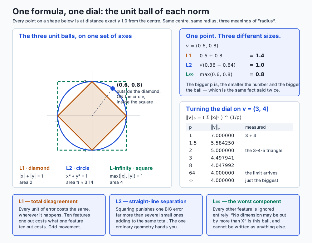
L1 gives a diamond: the points where |x| + |y| = 1. L2 gives the familiar circle. L-infinity gives a square: the points where the larger of |x| and |y| is 1. Their areas are 2, π and 4 — strictly increasing, which is the same fact as the falling column above said the other way round. A bigger p is a more forgiving norm, so more points fit inside its unit ball.
Take a single point, (0.6, 0.8), and measure it three ways. L1 says 0.6 + 0.8 = 1.4. L2 says √(0.36 + 0.64) = 1.0. L-infinity says max(0.6, 0.8) = 0.8. On the picture, that point sits outside the diamond, on the circle and inside the square. One point, three sizes, and you can see why.
The lab draws the same three balls as characters on a grid and counts the cells inside each — 469, 723 and 931 — which recovers the areas as 2.036, 3.138 and 4.041. Recognising π in a picture made of # and + is a pleasant sanity check that the shapes are what they claim to be.
Metrics, similarities, and the one that is neither
d(x, y) is a metric when it satisfies non-negativity, zero-only-at-zero, symmetry and the triangle inequality. The fourth is the one with teeth, and here is why you care: it is what lets an index skip whole regions of a dataset without opening them. If your query is 10 away from a cluster’s centre and the cluster has radius 2, nothing inside it can be closer than 8. That single deduction is the basis of ball trees, KD-trees, cover trees and every metric-space pruning scheme.
Day 103 proved that cosine distance is not a metric. Restated here with a triple you can hold in your head rather than a proof:
    cosine_distance(east, diagonal)  = 0.292893
    cosine_distance(diagonal, north) = 0.292893
    ----------------------------------------------
    going via the diagonal           = 0.585786
    cosine_distance(east, north)     = 1.000000   <-- LONGER
The direct route is 0.414214 longer than the detour. No metric may ever allow that. The lab goes further and sweeps every one of the 3375 triples of non-zero four-bit vectors: 326 of them violate the inequality. The same exhaustive sweeps over all 4096 triples find that Jaccard distance and Hamming distance never do.
Cosine distance fails a second axiom too, and this one bites more often in practice. cosine_distance((1, 0), (2, 0)) is 0 — distance zero between two things that are not the same thing. For cosine that is the feature: length is what it was asked to ignore. But it means cosine cannot tell a document from the same document repeated twice, and any deduplication built on it will not either.
The standard repair is worth knowing. Angular distance, arccos(similarity) / π, is a genuine metric on the same data and preserves the same ranking. Alternatively — and this is what vector databases actually do — normalise every vector to length 1 on the way in. Once ‖u‖ = ‖v‖ = 1, a single line of algebra gives
‖u - v‖² = 2 - 2·cos(u, v)so Euclidean distance and cosine similarity rank identically. You get cosine’s behaviour and a real metric, and the index is allowed to prune again. The practical advice is not “avoid cosine”; it is “normalise on the way in”.
Jaccard against cosine, on the same data
This is the pairing most people get wrong, because cosine is the habit. Take a query of four ingredients and two recipes:
| recipe | size | shared | union | Jaccard | cosine |
|---|---|---|---|---|---|
| Sachertorte | 11 | 4 | 11 | 0.3636 | 0.6030 |
| Shortbread | 3 | 2 | 5 | 0.4000 | 0.5774 |
Jaccard picks Shortbread. Cosine picks Sachertorte. Same two sets, same query, opposite answers, and both are defensible.
The arithmetic explains it in one line each. Cosine on binary vectors is shared / √(|query| · |recipe|), so 4 / √44 = 0.6030. Jaccard is shared / |union|, so 4 / 11 = 0.3636. Sachertorte contains every ingredient you named; cosine rewards that and charges only a square root for the seven extras, while Jaccard puts the extras in the denominator at full price.
Which is right depends on the question. “Has it got what I asked for?” is cosine. “Is it about the same size job?” is Jaccard. For duplicate detection, overlapping tag sets, shingled documents and anything where a long item must not out-rank a focused one, Jaccard is the safer default — and unlike cosine distance, 1 - Jaccard is a real metric.
There is a structural asymmetry underneath, and the lab checks it exhaustively over every pair of non-empty subsets of a six-element universe: cosine on binary data is never below Jaccard, because √(|a|·|b|) ≤ |a ∪ b| always. Cosine is systematically the more generous of the two on sets. If your relevance scores look suspiciously high, that is a candidate explanation before you go hunting for a bug.
Mahalanobis: Euclidean, after the data has had its say
Euclidean distance treats every direction as equally surprising. Real data does not.
Here are eight readings from two sensors that move together:
(-4, -3) (-3, -4) (-2, -1) (-1, -2) (1, 2) (2, 1) (3, 4) (4, 3)The mean is exactly (0, 0) and the population covariance comes out exactly
    [[7.5, 7.0],
     [7.0, 7.5]]
which you can check by hand: the variance of the first column is (16+9+4+1+1+4+9+16)/8 = 7.5, and the covariance is (12+12+2+2+2+2+12+12)/8 = 7.0. The correlation is 7.0/7.5 = 0.9333. The data has a grain: it runs along the line y = x.
Now take two probe points. (3, 3) — both sensors high together, an ordinary Tuesday. And (3, -3) — one sensor high while the other is low, which has never happened in this dataset. Both are √18 = 4.242641 from the mean, and Euclidean distance cannot tell them apart at all.
Mahalanobis can. The formula is one line: take the difference z, and instead of dotting it with itself, dot it with itself through the inverse covariance matrix.
d = √( z · (Σ⁻¹ z) )| probe | Euclidean | Mahalanobis |
|---|---|---|
| (3, 3) | 4.242641 | 1.114172 |
| (3, -3) | 4.242641 | 6.000000 |
A factor of 5.39 between two points that ordinary distance scores identically. An anomaly detector built on Euclidean distance has to give these the same score, and one of them is a sensor fault.
Where do 1.114172 and 6.0 come from? Day 106. Take the eigen-decomposition of that covariance matrix. The eigenvalues are 0.5 and 14.5; the eigenvector for 14.5 is the (1, 1) direction — along the grain, where the data spreads a lot — and the one for 0.5 is (1, -1), across it, where it barely spreads at all. Mahalanobis distance is Euclidean distance measured along those eigenvectors, with each component divided by the square root of its own eigenvalue:
    along  (3, 3)
      component along  (1, 1)/√2 = +4.242641   / √14.5 = +1.114172
      component across (1,-1)/√2 = +0.000000   / √ 0.5 = +0.000000
      hypotenuse                              = 1.114172

    across (3, -3)
      component along  (1, 1)/√2 = +0.000000   / √14.5 = +0.000000
      component across (1,-1)/√2 = +4.242641   / √ 0.5 = +6.000000
      hypotenuse                              = 6.000000
So Mahalanobis is not a new kind of distance. It is Euclidean distance in the coordinate system the data chose for itself, and Day 106’s eigenvectors are the axes of that system. Substitute the identity matrix for Σ⁻¹ and you get ordinary Euclidean distance back exactly — which is the cleanest statement of what the covariance is doing. It is the thing that would be the identity if every feature had variance 1 and no feature had anything to do with any other. Real data is never that, and Euclidean distance quietly assumes it always is.
The cost is real and worth stating. Mahalanobis needs an invertible covariance matrix, which needs more rows than columns and no two features that are exact duplicates. It needs re-estimating when the data drifts. And a singular covariance must fail loudly rather than return a plausible number — the lab’s implementation raises on [[1, 2], [2, 4]].
The thing that silently decides your answer
Everything above assumed the columns were comparable. They usually are not.
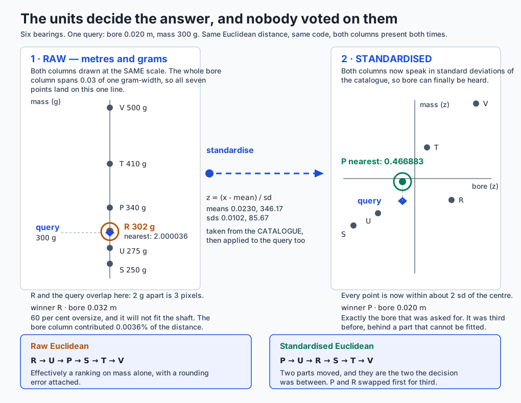
A bearing catalogue with two features, recorded in whatever units the supplier used: bore diameter in metres and mass in grams. The query wants a 0.020 m bore and 300 g. Rank on raw Euclidean distance:
    part          distance       bore term       mass term   bore share
    R             2.000036        1.44e-04            4.00   0.003600%
    U            25.000001        3.60e-05          625.00   0.000006%
    P            40.000000        0.00e+00         1600.00   0.000000%
Look at the last column. The bore diameter contributes less than one ten-thousandth of one per cent of every distance in the table. This is not a ranking on two features; it is a ranking on mass with a rounding error attached. And the winner, R, has a 32 mm bore where 20 mm was asked for — 60 per cent oversize, a part that will not fit the shaft. It wins because it is 2 g from the target mass. P, which has exactly the bore requested, comes third.
Standardise both columns — subtract the column mean, divide by the column standard deviation — and re-run the identical code:
    part        bore (z)    mass (z)      distance
    P            -0.2928     -0.0720      0.466883
    U            -0.8783     -0.8307      0.654221
    R             0.8783     -0.5155      1.171313
The winner changed from R to P. Two of the six parts moved, and they are the two the decision was between: P and R swapped first for third.
The clearest proof that the raw ranking was an artefact is to change no data at all — only the unit one column is written in:
    bore in metres        ['R', 'U', 'P', 'S', 'T', 'V']
    bore in millimetres   ['R', 'U', 'P', 'S', 'T', 'V']
    bore in micrometres   ['P', 'U', 'T', 'R', 'S', 'V']
The parts did not change; a column header did. Any pipeline that does not normalise is letting whoever chose the units decide the ranking, and that person was not thinking about distances.
Two details worth carrying. First, standardise the query with the catalogue’s means and standard deviations, not its own — a single row standardised against itself is a row of zeros, which is exactly the mistake scikit-learn’s fit/transform split exists to prevent. Second, this is not a property of six hand-picked rows: the lab runs 2000 random catalogues from a seeded generator and the winner changes after standardising in 1090 of them, about 55 per cent.
One more warning, because “cosine is scale invariant” is repeated far too confidently. Cosine ignores the length of a vector. It does not ignore the units of a column, and it cannot, because changing one column’s units rotates every vector in the table. The lab checks both halves: doubling every candidate vector leaves the cosine ranking untouched to within 1e-12, and changing the bore column from metres to micrometres changes it.
An everyday analogy
Think of a city, and of the question “how far is the station from here?”
Ask a taxi driver. She answers in blocks: four across and three up is seven blocks, because she cannot drive through buildings. Every block costs the same wherever it is. That is L1, and her answer is not an approximation of anything — for a taxi, it is exact.
Ask a pigeon. It answers five, because it flies the diagonal. That is L2, and it is the only one of these that is a physical length.
Ask the site foreman running a gantry crane on two rails. He answers four, because the two motors run at once and the job finishes when the slower axis finishes. That is L-infinity, and it is the only one that predicts his schedule.
Three answers, one displacement, nobody wrong. That is the whole family, and it is why “which is the real distance” is not a question with an answer until you have said who is travelling.
Now extend it. Ask “how far is that shop from this shop”, where the shops are described not by position but by what they sell. Two shops that stock exactly the same twelve things are the same shop for your purposes, even if one is in a different postcode — that is cosine, throwing away magnitude and keeping direction. A corner shop stocking four of your twelve, and a department store stocking all twelve plus four hundred others: cosine likes the department store, because everything you wanted is there. Jaccard likes the corner shop, because most of what it sells is what you wanted. Both are reasonable shopping advice; they are advice about different trips.
Then there is the part of the analogy that Mahalanobis supplies, and it is the one that changes how people think. In a real city, “one kilometre” is not one thing either. A kilometre along the motorway is nothing; a kilometre across a river with no bridge is a serious journey. Locals know this and route accordingly, not by measuring the map but by knowing where the city flows. Mahalanobis distance is what you get when you let the data tell you where it flows — along the grain is cheap, across it is expensive — and Day 106’s eigenvectors are the roads.
The analogy has one leak, and it is worth naming rather than hiding: in a city the geography is fixed, while a covariance matrix is estimated from the data you happen to have. Add a few readings across the grain and the “river” narrows. That is a real difference, and the security section returns to it.
Examples in practice
Text and semantic retrieval — cosine, almost always. Documents vary enormously in length, and length is exactly what you want to ignore: a 5,000-word article on norms and a 500-word note on norms are about the same thing. In the opening example, Cartogram is the query’s profile at three times the length and scores a cosine of exactly 1.0 while sitting further away in L2 than anything else on the page. Every vector database defaults to cosine or to inner product on normalised vectors for this reason, and the reason is not that cosine is better in the abstract.
Recommenders and basket analysis — Jaccard, more often than people use it. “Customers who bought this also bought” is set overlap. Cosine here systematically favours the customer with three hundred purchases, because it charges only a square root for their other 296 items. If your recommendations are dominated by generically popular items, that is worth checking before you reach for a re-ranker.
Tabular models and clustering — Euclidean, after scaling, or Mahalanobis instead. k-means is defined in terms of squared Euclidean distance and cannot be given a different measure without changing what it converges to. That makes scaling non-optional rather than advisable: the bearing catalogue above is what k-means sees when you skip it.
Categorical features — Hamming, and the mistake to avoid. The integer-encoding trap earlier is not hypothetical; it is what happens when a categorical column survives a LabelEncoder and goes straight into a distance-based model. One-hot encoding plus Hamming, or Gower distance for mixed tables, is the honest route. Note the pleasant coincidence the lab measures: on binary features, Hamming, L1 and squared L2 are all the same number, because every difference is 0 or 1 and 1 squared is 1. That coincidence is worth knowing and worth distrusting, because it evaporates the moment the encoding is integers rather than bits.
Anomaly detection and quality control — Mahalanobis and Chebyshev. Mahalanobis is the standard multivariate outlier score precisely because of the two-probe example above. Chebyshev is what a tolerance specification already is, whether or not anyone has written it that way.
Embedding spaces at scale — everything above, plus the curse. Day 103 introduced the curse of dimensionality: as dimensions grow, the ratio of the nearest to the farthest distance approaches 1 and “nearest neighbour” stops meaning much. It hits the p-norms unevenly, and lower p degrades more slowly — which is a genuine argument for L1 in high dimensions and one that is easy to test yourself. The lab’s fifth extension exercise sets it up.
Implications: security, privacy, performance, scalability, and cost
Security. A distance function is an access-control decision in disguise whenever it is used for matching. Face matching, fingerprint matching, deduplication, fraud-ring detection, “is this login from a familiar device” — every one is a threshold on a distance, and every one inherits whatever the measure was told to ignore.
Three consequences follow directly from this day’s material. Cosine similarity cannot distinguish a document from the same document repeated, which the lab asserts as cosine_distance((1, 0), (2, 0)) == 0; a plagiarism or dedup check built on cosine over raw counts inherits that hole. An unscaled feature is a published map of which field to manipulate — if one column contributes 99.99 per cent of the distance, an attacker needs to control exactly one column. And Mahalanobis depends on an estimate: an adversary who can inject rows can widen the variance in the direction they intend to attack along, and their own anomaly score drops afterwards. Any detector that re-fits its covariance on live traffic without provenance controls has that property.
Privacy. Distances leak. Publishing pairwise distances between records is not anonymisation: with enough of them, multidimensional scaling reconstructs the geometry, and with a few known points it reconstructs positions. “We only shared the similarity matrix” is a sentence that has preceded several re-identification results. The same caution applies to exposing raw similarity scores through an API, which is an oracle an attacker can query.
Performance. The measures differ by more than a constant. L1 needs an absolute value per dimension; L2 needs a multiply and, if you actually take the root, a square root — which is why so much code ranks on squared distance and why that is legitimate for ranking and illegitimate for anything that needs the triangle inequality. Cosine needs two norms as well as the dot product, unless you normalise once at write time and store unit vectors, which turns every subsequent comparison into a plain dot product. That is the single biggest constant-factor win available in a retrieval system, and it is free.
Mahalanobis is the expensive one, and it is worth knowing where the cost sits. Inverting the covariance is O(d³) and happens once; each subsequent distance is a matrix-vector product, O(d²) rather than O(d). In 1000 dimensions that is a thousandfold increase per comparison, which is why Mahalanobis is common in tens of dimensions and rare in embedding spaces. The usual compromise is a diagonal covariance, which is exactly per-feature standardisation and costs nothing extra.
Scalability. This is where the metric axioms turn into money. A metric permits tree-based pruning, so a query need not touch most of the dataset. A non-metric does not, and the honest options are brute force, an approximate index whose guarantees are empirical rather than proved, or normalising to make Euclidean distance apply. The last is why “normalise on the way in” is the standard advice and not merely a tidiness preference.
Cost. The concrete bill is the one at the top of this lesson. A vector index is built for a chosen metric, and changing it means rebuilding — for a large corpus, hours of compute and, on managed services, a real invoice. The cheap moment to think about the measure is before the first index is created; the expensive moment is after a relevance complaint six months later.
Alternatives: free, open source, and commercial
Everything named here is free and open source. There is no paid tier for any of it, and none of it needs an account or a key. The commercial products in the area — managed vector databases — charge for hosting and operations, not for the distance functions, which are the same handful of formulas everywhere.
NumPy’s linalg.norm — used here, and it is the p-norm family. Its ord parameter is p. ord=1, ord=2 and ord=np.inf are L1, L2 and Chebyshev, and any float in between works too.
import numpy as np
d = np.asarray(query) - np.asarray(candidate)
np.linalg.norm(d, ord=1)       # Manhattan
np.linalg.norm(d, ord=2)       # Euclidean
np.linalg.norm(d, ord=np.inf)  # Chebyshev
np.linalg.norm(d, ord=1.5)     # anywhere in between
Choose it when you are already in NumPy and want one distance at a time, or a whole column of them with axis=. On the authoring machine it agreed with the from-scratch implementation in the lab to within 1e-12 on every p tested, and this is the tool the lab actually ran. Two traps worth knowing: ord=0 counts the non-zero entries, which is genuinely useful for measuring sparsity and is not a norm — doubling a vector does not change how many entries are non-zero, so absolute homogeneity fails; and negative ord values are accepted and are not norms either.
SciPy’s scipy.spatial.distance — the standard toolbox. Not installed on the authoring machine, so no output is reproduced for it here; the description is from its documentation. It provides the individual functions (cityblock, euclidean, chebyshev, minkowski, cosine, hamming, jaccard, mahalanobis, canberra, braycurtis and more), plus the two that matter at scale: cdist(XA, XB, metric=...) for every pair between two collections, and pdist(X, metric=...) for every pair within one, returned in condensed form. Choose it when you need a matrix of distances rather than one, or when you need a metric NumPy does not have. Two documented behaviours to note before you swap it in: scipy.spatial.distance.hamming returns the fraction of differing positions rather than the count, and its jaccard operates on boolean arrays.
scikit-learn’s pairwise_distances — the one that scales. Not installed here either, and no output is reproduced. Same idea as cdist with two additions that matter in practice: n_jobs for parallelism, and metric="precomputed" so that estimators such as DBSCAN, AgglomerativeClustering and KNeighborsClassifier accept a distance matrix you computed yourself with any measure at all — including one of your own. That is the escape hatch when a library’s built-in metrics do not include what your data needs. sklearn.preprocessing.StandardScaler is the standardisation from this lesson, with the fit/transform split that prevents the query-standardised-against-itself bug, and it uses the population divisor n, which is what this lab’s column_stds matches.
Vector databases — the metric as a creation-time decision. Not exercised here; described from documentation. FAISS (open source, from Meta) exposes IndexFlatL2 and IndexFlatIP for inner product, with cosine obtained by normalising vectors before insertion. pgvector (open source, a PostgreSQL extension) exposes L2, inner product, cosine, L1, Hamming and Jaccard distance through distinct operators, and the index you build must match the operator you query with. Qdrant, Weaviate, Milvus and Chroma are all open source and all take the metric as a collection-creation parameter. The pattern is the same everywhere and it is the practical reason this day exists: the metric is chosen when the index is created, and changing it means rebuilding.
Writing it yourself — always available, and often right. The measures are three to ten lines each. The lab writes seventeen of them with abs, sum, max and math.sqrt. Choose that when you need a measure nobody ships (a weighted mix, a domain-specific edit distance, a cost matrix over categories), when the dependency is not worth it, or when — as here — the point is to know what the library is doing.
Comparison with related concepts
| Measure | Distance or similarity | A metric? | Right when | Wrong when |
|---|---|---|---|---|
| L1 / Manhattan | distance | yes | Movement is axis-by-axis; you want total disagreement; high dimensions | One big error should cost more than several small ones |
| L2 / Euclidean | distance | yes | Real geometry; one large error must dominate; features already comparable | Features in mismatched units, or heavily correlated |
| L-infinity / Chebyshev | distance | yes | A tolerance rule; the slowest axis sets the time | Every feature should contribute |
| Cosine similarity | similarity | no | Direction matters and magnitude does not: text, embeddings | Magnitude is information — counts, prices, quantities |
| Hamming | distance | yes | Categorical or binary fields with no ordering | Values have a real numeric ordering |
| Jaccard | similarity | 1 − it is a metric | Sets of differing sizes; overlap, deduplication | Repeat counts matter, not just presence |
| Mahalanobis | distance | yes, given a fixed Σ⁻¹ | Correlated features, mixed units, outlier scoring | d is large, rows are few, or the covariance is singular |
| Squared Euclidean | neither | no | Ranking only, where the root is wasted work | Anything assuming the triangle inequality |
Two distinctions people conflate, worth separating explicitly.
Similarity is not “one minus distance”. Cosine similarity runs from −1 to 1 and 1 − cosine is bounded and well behaved, so that particular conversion is fine. Euclidean distance is unbounded, so 1 − d goes negative and 1/(1+d) is a choice, not a derivation. Any time you convert between the two you have added a modelling assumption; write it down.
Standardising is not the same as what Mahalanobis does. Standardising rescales each column independently. Mahalanobis also removes the correlation between columns. On the bearing catalogue, where bore and mass correlate at +0.7979, the two give different answers: standardised Euclidean ranks P first, Mahalanobis on the raw numbers ranks U first and P second. Both demote the unusable part R — from first to third and from first to fifth respectively — but they disagree at the top, and the disagreement is not noise. Once you know that heavier goes with wider in this catalogue, being heavy-for-its-bore is the surprising thing, and U, which is smaller and lighter together, reads as the nearer part. Whether you want that is a modelling decision, which is this day’s entire subject.
That last result is worth flagging as a correction. It is natural to expect Mahalanobis to reproduce the standardised ranking, since both are cures for the same disease. On this catalogue it does not, and the reason is the correlation term. The lab asserts the ranking it actually measured rather than the one that would have made a tidier sentence.
When to use it — and when not to
Choose by the shape of the data, not by the name of the measure.
| The data looks like | Reach for | Because |
|---|---|---|
| Text, embeddings, anything where length varies but topic is the point | Cosine, or L2 on unit-normalised vectors | Direction carries the meaning; length is an artefact of how much was written |
| Sets: tags, baskets, shingles, species lists | Jaccard | Charges for what is not shared, in both directions, so a long item cannot out-rank a focused one |
| Categorical fields with no ordering | Hamming | Counts differences without inventing an ordering that is not there |
| Binary flags | Hamming, L1 or squared L2 — they agree exactly | Every difference is 0 or 1, and 1 squared is 1 |
| Numeric features, comparable units, roughly independent | Euclidean | The straightforward answer, and here it is the right one |
| Numeric features in mismatched units | Standardise, then Euclidean | Otherwise the column with the bigger numbers decides alone |
| Numeric features that are correlated | Mahalanobis | Removes the shared movement as well as the scale |
| Movement is constrained to axes | Manhattan | The diagonal is a distance you cannot travel |
| The rule is “no single feature worse than X” | Chebyshev | That rule already is an L-infinity ball |
| Very high dimensions | Lower p; consider L1 | The curse degrades higher p faster |
And the cases where the popular answer is wrong:
Do not use cosine when magnitude is information. Prices, counts, quantities, dosages. Cosine will happily tell you that a basket of 2 items and a basket of 200 in the same proportions are identical.
Do not use Euclidean on unscaled mixed-unit features. This is the single most common failure in the list, it produces no error message, and the bearing example above is what it looks like.
Do not use a non-metric where a metric is assumed. Ball trees, cover trees, metric-space pruning, and the termination proof for k-medoids all need the triangle inequality. Normalise and use Euclidean, or use angular distance.
Do not use Mahalanobis when you cannot estimate the covariance. More features than rows, or two features that are duplicates, and the matrix is singular. A shrinkage estimator or a diagonal covariance is the honest fallback; the diagonal case is exactly per-feature standardisation.
Do not encode categories as integers and reach for Euclidean. It is fast, it runs, and it asserts an ordering that does not exist.
Do not put squared Euclidean distance anywhere that needs a distance. Ranking, yes. Anything else, no.
Finally, a heuristic that is worth more than any of the above: if you cannot say in one sentence what question your measure is asking, you have not chosen it yet. “Total disagreement across the features.” “Is any single feature badly wrong.” “Same mix, any size.” “How many fields differ.” “How much of everything involved is shared.” “How surprising is this, given how the data usually behaves.” If none of those is the sentence you want, the measure is not one of these.
Knowledge check
Take the quiz for this day. Eight questions, and two of them are the ones worth getting right: why cosine distance is not a metric — and what, specifically, breaks as a result — and what standardising actually changes about a ranking. If either of those is fuzzy, re-read “Metrics, similarities, and the one that is neither” and “The thing that silently decides your answer” before moving on.
Hands-on exercise
The lab is “Choose Your Distance on Purpose”. Set it up:
cd labs/sections/math-statistics-and-data/day-107-norms-distances-and-similarity-measures
python3 -m venv .venv
.venv/bin/pip install -r requirements/requirements.txt
.venv/bin/python3 -c "import numpy; print(numpy.__version__)"
Then read starter/00_brief.md and work through starter/measures.py — seventeen functions in pure Python, standard library only — and starter/answers.py, twenty-five predictions to write down before you run anything.
The order that hurts least: the three norms first, then the general p_norm, then the three distances and cosine, then Hamming, Jaccard and the binary-vector helper, then rank. Everything above becomes visible the moment rank works. Finish with the statistics: column_means, column_stds, standardise, covariance_matrix and mahalanobis_distance.
Check yourself at any point, from the lab directory:
.venv/bin/pytest starter -qExpected output
On an untouched checkout:
1 passed, 71 skippedUnattempted work is skipped, not failed. When it says 72 passed, you are finished.
The reference scripts, run afterwards, produce the numbers this lesson quotes. The opening disagreement:
    L1 (Manhattan)       picks  Aisle
    L2 (Euclidean)       picks  Beacon
    L-inf (Chebyshev)    picks  Beacon
    cosine similarity    picks  Cartogram
The three unit balls, drawn as characters — # inside the L1 diamond, + out to the L2 circle, . filling the corners of the L-infinity square:
          ................+++++++###+++++++................
          ...........+++++++++#########+++++++++...........
          ......+++++++++###################+++++++++......
          ..++++++#################################++++++..
          #################################################
          ..++++++#################################++++++..
          ......+++++++++###################+++++++++......
          ...........++++++++++#######++++++++++...........
          ................+++++++###+++++++................
The two probes that Euclidean distance cannot separate:
    probe            Euclidean   Mahalanobis
    (3.0, 3.0)        4.242641      1.114172
    (3.0, -3.0)       4.242641      6.000000
And the full harness:
98 checks, 0 failure(s).Validate your work
-
The install printed
2.5.2. -
.venv/bin/pytest examples -qprints105 passed. -
.venv/bin/pytest starter -qprints1 passed, 71 skippedbefore you start and72 passedwhen you finish. -
Each of the six reference scripts exits 0 and ends with
NN_name.py: every assertion held. -
bash tests/run_tests.shprints98 checks, 0 failure(s).and exits 0. Check the exit status directly rather than through a pipe:bash tests/run_tests.sh; echo "exit=$?" -
Your own output matches
expected-output/, allowing for the machine-dependent fields named inexpected-output/FIELDS.md.
Troubleshooting
p_norm returns inf at p = math.inf. You computed the limit as arithmetic. 4.0 ** math.inf is inf. Handle the infinity case with math.isinf(p) and return the largest absolute component.
ValueError: max() arg is an empty sequence. max(()) raises where sum(()) returns 0. Pass default=0.0. An empty vector is not exotic — it is what a feature extractor returns for a document containing none of your vocabulary.
column_stds is about 9 per cent off NumPy’s. You divided by n - 1. This lab uses the population divisor n, which is what numpy.std does by default and what scikit-learn’s StandardScaler uses.
Every standardised value came out zero. You standardised the query against itself. Compute the means and standard deviations from the catalogue and pass them in.
math domain error inside mahalanobis_distance. The value under the square root should be exactly 0 and came out around -1e-17. Clamp a tiny negative to 0 — but raise for one that is genuinely negative, because that means the matrix you were handed is not an inverse covariance. Do not use abs; it would turn a real error into a plausible number.
The two Mahalanobis routes disagree in the last digit. They are supposed to. The lab’s Gauss-Jordan inverse gives exactly 6.0 and numpy.linalg.inv gives 5.999999999999999, a difference of 8.882e-16. Both are correct; IEEE 754 addition is not associative. This is why every comparison in the lab states a tolerance.
troubleshooting.md in the lab covers the rest.
Common mistakes
- Sorting a similarity ascending.
cosine_similarityandjaccard_similaritygrow as things get more alike; everything else here shrinks. Get it backwards and the worst match arrives at the top with no error anywhere. This is the most consequential bug in the lab, andranktakes an explicithigher_is_betterflag so that the choice has to be made rather than assumed. - Zipping two vectors of different lengths.
ziptruncates silently, so you get an answer to a question you did not ask. The lab’s_pairedraises instead. - Returning 0.0 for the cosine of a zero vector. It has no direction; the answer is undefined. Raise.
- Breaking ranking ties by dictionary order. Two candidates that score exactly equal will swap between runs. Sort on a tuple so ties fall back to the name.
- Patching
p < 1through. The formula still returns a number belowp = 1and that number is not a norm. Refuse it.
Practice assignment
Take a dataset of your own — one you already have, with at least four features and at least one non-numeric column — and write a one-page measure decision record for it. Not an essay; a record you would put in a repository.
It must contain:
- A table of your features, each with its type (numeric, categorical, binary, set-valued), its units, and its observed range. The units column is the one that does the work.
- The question you are asking, in one sentence, in the form of one of the six sentences from the end of “When to use it — and when not to”. If none of them fits, write your own and say why the six do not.
- Your chosen measure, and two you rejected, each with a sentence saying what it would have got wrong on your data.
- Evidence, computed by you. Rank the same five candidates against the same query under all three measures, using the lab’s
rankwith the measure as a parameter, and paste the three orderings. If they agree, say so — that is a real result and it means the choice matters less than you feared. - A before-and-after scaling check. Rank once on raw values and once after standardising, and report whether the top result changed. If your features are already in the same units, say that and say why it is safe.
- The metric question. Is your measure a metric? If not, name the axiom it fails and the thing downstream that was relying on it — an index, a clustering algorithm, a proof, or nothing.
Two guardrails so the exercise stays honest. State a tolerance for every float you compare, and use a fixed seed if any part of it is random. And if the three orderings turn out identical, do not go looking for a dataset where they differ; report what you found. A dataset where the measure does not matter is worth knowing about, and it is not a failed assignment.
Extension challenge
Five, in rough order of difficulty. The first three are in the lab’s own extension list with full setups.
1. Draw the ball for p = 0.5. p_norm refuses it, and the refusal deserves evidence. Relax the guard in a copy, render the “unit ball” on the character grid from script 02, and find a concrete triple that breaks the triangle inequality on the four-pointed star you get. You will then have proved the guard right rather than taken it on trust.
2. Poison a covariance. Add rows to the sensor dataset that lie across the grain, recompute the covariance, and watch the Mahalanobis distance of (3, -3) fall from 6.0. How many injected rows does it take before the anomaly scores as normal? That number is the one a security review would want, and it is the concrete form of the caution in this lesson’s Implications section.
3. Measure the curse. Generate random points in 2, 10, 100 and 1000 dimensions and plot the ratio of the nearest to the farthest distance under L1, L2 and cosine. One of the three degrades much more slowly than the others. Day 103 introduced the curse as a warning; this turns it into a graph you made.
4. Build a weighted Mahalanobis by hand. A diagonal matrix in the Mahalanobis formula is exactly a per-feature weighting. Set the weights deliberately — “bore diameter matters ten times as much as mass” — and compare the resulting ranking with the standardised one and with the full-covariance one. You now have three defensible answers and a reason to prefer one, which is the position this day is trying to get you to.
5. Implement one metric nobody shipped. Pick a domain measure that no library provides: a cost matrix over your categories where “steel to brass” genuinely is cheaper than “steel to nylon” because you have a substitution table; or a weighted Jaccard where rare tags count for more. Then check the four metric axioms numerically the way script 03 does, exhaustively if your space is small enough. Most home-made measures fail one. Finding out which — before an index is built on it — is the whole skill this day is for.
The AI thread
Every retrieval system, every clustering algorithm and every nearest-neighbour classifier has a distance function inside it, and it is the hyperparameter people most reliably leave at the default.
Think about how much rests on it. Retrieval-augmented generation is a distance computation followed by a language model: the model can only reason over what the retrieval step handed it, so the measure decides what the model is allowed to know. A recommender is a distance over user or item vectors. Anomaly detection is a threshold on a distance. Semi-supervised learning propagates labels along a graph built from distances. Even the loss functions are norms — L2 loss is the Euclidean norm of the residual, L1 loss is the Manhattan norm, and the reason L1 regularisation produces sparse models while L2 does not is precisely the diamond in this lesson’s first diagram: the diamond has corners on the axes, and a corner is where a coefficient becomes exactly zero. Ridge and lasso are not two unrelated tricks. They are the same idea with the dial set to 2 and to 1.
So the practical thread is short and it is the reason today exists. First: say the sentence. If you cannot state in one line what question your measure is asking, you have not chosen it, and something else has chosen for you. Second: check the units before you check anything else. The bearing catalogue in this lesson is not a contrived example; it is what an unscaled feature table looks like from the inside, and the failure is silent, plausible and confidently wrong. An unscaled feature is a thumb on the scale that nobody put there on purpose and nobody can see in the output.
And the third, which is the one that will save you a rebuild: decide the measure before the index exists. It is one line in a configuration file on the first day and hours of recomputation six months later. That asymmetry is the whole practical argument for spending a day on a family of formulas that each fit on one line.
Quiz
Q1. One query and three candidate articles, four term counts each. Manhattan distance ranks the first article top, Euclidean ranks the second, and cosine similarity ranks the third. Which statement is correct?
- Two of the three implementations must contain a bug, because the same data cannot have three nearest neighbours
- All three are correct; they are answering different questions, and which one you want is a modelling decision
- Cosine is the only correct answer, because the other two are sensitive to document length
- The disagreement means the features are badly chosen and the vectors should be re-derived
Show answer
Answer: B. All three are correct; they are answering different questions, and which one you want is a modelling decision
Nothing is broken. Manhattan asks "how much total disagreement is there across the features", and the first article disagrees on one term by 5, total 5. Euclidean squares before summing, so one error of 5 costs 25 while three errors of 2 cost 12 in total — which is why it prefers the second article despite its larger total. Cosine throws length away entirely, so the third article, which is the query profile at exactly three times the length, scores 1.0 while being the furthest away of the three under both L1 and L2. The first option assumes there is a fact of the matter about which is nearest, and there is not until you say what near means. The third gets the reasoning backwards: cosine is often right for text precisely because it ignores length, but ignoring length is wrong whenever magnitude is information, such as prices or counts. The fourth blames the representation for a property of the measure; the same three vectors under any one measure give one clean answer.
Q2. Why is cosine distance not a metric?
- It can return negative values, which violates non-negativity
- It is not symmetric: the distance from A to B differs from the distance from B to A
- It violates the triangle inequality, and it is zero between vectors that are not equal
- It is undefined for the zero vector, which violates the requirement that every pair have a distance
Show answer
Answer: C. It violates the triangle inequality, and it is zero between vectors that are not equal
Two of the four axioms fail, and both are worth knowing. The triangle inequality: with east = (1, 0), diagonal = (1, 1) and north = (0, 1), going east to diagonal costs 0.292893 and diagonal to north costs the same, so the detour totals 0.585786 — while going east to north direct costs 1.0. A detour shorter than the direct route is exactly what no metric may allow, and an exhaustive sweep over the 3375 triples of non-zero four-bit vectors finds 326 violations. The second failure is identity of indiscernibles: cosine_distance((1, 0), (2, 0)) is 0, so two different vectors are at distance zero. For cosine that is the feature rather than a defect — length is what it was told to ignore — but it means cosine cannot distinguish a document from the same document repeated. The first option is wrong for non-negative data, where cosine similarity lies in 0 to 1 and the distance in 0 to 1; on data with negative components the similarity can reach -1 and the distance 2, which is still non-negative. The second is simply false: the formula is symmetric in its two arguments. The fourth describes a real edge case but not an axiom violation, since the axioms concern points that exist in the space. What the failure costs you is concrete: ball trees, KD-trees, cover trees and metric-space pruning all rely on the triangle inequality, so none of them is valid. The standard repairs are angular distance, arccos of the similarity divided by pi, or normalising every vector to length 1 so Euclidean distance ranks identically.
Q3. A machined part has four dimensions and is rejected if any single dimension is out by more than 0.05 mm. Batch A is out by 0.04 on all four; batch B is exact on three and out by 0.09 on the fourth. Which measure expresses the acceptance rule, and which batch passes?
- Chebyshev, and batch A passes
- Manhattan, and batch B passes
- Euclidean, and batch A passes
- Chebyshev, and batch B passes
Show answer
Answer: A. Chebyshev, and batch A passes
The rule "no single feature may be worse than X" is an L-infinity ball and cannot be written as anything else. Batch A worst deviation is 0.04, which is inside the 0.05 tolerance, so it passes; batch B worst is 0.09, so it fails. Now look at what the other two measures say. Batch A total absolute error is 0.16 and batch B is 0.09, so Manhattan ranks batch B as the better part. Euclidean gives 0.0800 for A and 0.0900 for B, so it ranks A better — the two disagree with each other here, which is itself worth noticing. Neither is answering the inspection question. The general lesson is that averaging, whether L1 or L2, is a way of hiding one bad value behind several good ones, and whenever the specification is about a worst case, the measure has to be too.
Q4. You are matching recipes by ingredient set. The query lists four ingredients. Sachertorte has eleven ingredients including all four; Shortbread has three ingredients, two of which are in the query. Cosine similarity prefers Sachertorte and Jaccard prefers Shortbread. Why?
- Jaccard is computed on counts while cosine is computed on presence, so they see different data
- Cosine divides by the square root of the two set sizes while Jaccard divides by the size of the union, so Jaccard charges full price for the seven extra ingredients
- Cosine is a distance and Jaccard is a similarity, so their orderings are naturally reversed
- Jaccard is undefined for sets of different sizes and is falling back to a default
Show answer
Answer: B. Cosine divides by the square root of the two set sizes while Jaccard divides by the size of the union, so Jaccard charges full price for the seven extra ingredients
Both are computed on exactly the same binary data, and the difference is entirely in the denominator. Cosine on binary vectors is shared over the square root of the product of the sizes, so 4 over the square root of 44, which is 0.6030. Jaccard is shared over the union, so 4 over 11, which is 0.3636. For Shortbread the numbers are 2 over the square root of 12, or 0.5774, and 2 over 5, or 0.4000. A square root is a much gentler penalty than a full count, so cosine forgives the seven extra ingredients and Jaccard does not. Neither is wrong: cosine is answering "has it got what I asked for" and Jaccard is answering "how much of everything involved is shared". The first option has it backwards; both are computed on presence here, and it is Jaccard that is defined on sets from the start. The third is false in a way worth correcting, since both cosine similarity and Jaccard similarity are similarities and both are being maximised. The fourth is simply untrue: Jaccard was invented in 1901 precisely for lists of very different lengths. One structural fact follows and is worth carrying: on binary data, cosine can never score below Jaccard, because the square root of the product of two sizes is never larger than the size of their union. Cosine is systematically the more generous of the two.
Q5. Two points sit at exactly the same Euclidean distance from the mean of a dataset, and Mahalanobis distance scores one at 1.11 and the other at 6.00. What has Mahalanobis used that Euclidean has not?
- A larger number of dimensions, since Mahalanobis operates in a higher-dimensional space
- The covariance of the data, so that moving along the direction the data varies in is cheap and moving across it is expensive
- A weighting supplied by the user, which Euclidean distance does not accept
- The median rather than the mean, which is more robust to outliers
Show answer
Answer: B. The covariance of the data, so that moving along the direction the data varies in is cheap and moving across it is expensive
Mahalanobis distance is the difference dotted with itself through the inverse covariance matrix rather than with itself directly. On the eight sensor readings in the lab, the two sensors move together — the covariance is [[7.5, 7.0], [7.0, 7.5]] and the correlation is 0.9333 — so the data has a grain running along the line y = x. Both sensors reading 3 is ordinary; one reading +3 while the other reads -3 has never happened. Euclidean distance has no way to know that, because it does not know the dataset exists; both probes are the square root of 18 from the mean and it must score them identically. Day 106 supplies the connection: the eigenvalues of that covariance are 0.5 and 14.5, the eigenvector for 14.5 is the (1, 1) direction and the one for 0.5 is (1, -1), and Mahalanobis is Euclidean distance along those axes with each component divided by the square root of its eigenvalue. That is where 1.114172 and exactly 6.0 come from, and you can do the arithmetic by hand. The first option is wrong: both operate in the same two dimensions. The third describes a diagonal weight matrix, which is a special case of Mahalanobis and is exactly per-feature standardisation — the general case learns the weights and the correlations from the data instead. The fourth is a different idea altogether; Mahalanobis uses the mean.
Q6. A catalogue has two features: bore diameter in metres, around 0.02, and mass in grams, around 350. You rank on raw Euclidean distance and then again after standardising both columns. What changes?
- Nothing changes; standardising is a monotonic transformation and monotonic transformations preserve rankings
- The distances all shrink but the ordering is preserved, which is why standardising is described as cosmetic
- The ordering changes, because before standardising the bore column contributed a negligible fraction of every distance
- The ordering changes only if the features are correlated; for independent features standardising has no effect
Show answer
Answer: C. The ordering changes, because before standardising the bore column contributed a negligible fraction of every distance
Before standardising, the squared bore differences are around 1e-4 and the squared mass differences are in the thousands, so the bore column contributes at most 0.0036 per cent of any distance in the table. That is not a two-feature ranking; it is a ranking on mass. The winner is a bearing whose bore is 60 per cent oversize and physically will not fit, and it wins because it is 2 g from the target mass. After both columns are divided by their own standard deviations the winner changes, and the two parts that move are exactly the two the decision was between. The first two options both misunderstand what standardising does: it is applied per column with a different divisor for each, so it is not one monotonic transformation of the distance and there is no reason for the ordering to survive. The fourth confuses standardising with Mahalanobis; correlation is what Mahalanobis additionally removes, while standardising fixes only the scale — and the scale alone is enough to decide this ranking. The sharpest demonstration is that changing no data at all and only the unit the bore column is written in, from metres to micrometres, also changes the winner. Over 2000 random catalogues with a seeded generator, standardising changed the winner about 55 per cent of the time.
Q7. Why is squared Euclidean distance not a norm or a metric, and when is it nevertheless safe to use?
- It fails non-negativity; it is safe only when all features are positive
- It fails symmetry; it is safe when the two arguments are always supplied in the same order
- It fails nothing; it is a norm, and the square root is dropped purely as an optimisation
- It fails absolute homogeneity — doubling a vector quadruples it — and is safe for ranking, because squaring preserves order on non-negative numbers
Show answer
Answer: D. It fails absolute homogeneity — doubling a vector quadruples it — and is safe for ranking, because squaring preserves order on non-negative numbers
Absolute homogeneity requires that scaling a vector by k scales its size by the absolute value of k. For v = (3, -4, 12) the sum of squares is 169, and for 2v it is 676 — four times, not twice — so the axiom fails outright and the triangle inequality goes with it. That does not make it useless. Squaring is monotonic on non-negative numbers, so ranking by squared distance gives exactly the same order as ranking by Euclidean distance, which the lab asserts directly, and skipping the square root is a real saving inside a tight loop. What it makes it is unusable as a distance: never hand it to a ball tree, a cover tree, a metric-space index, or any argument that relies on a detour being no shorter than the direct route. The first option is wrong because a sum of squares is never negative. The second is wrong because the expression is symmetric in its two arguments. The third is the belief the question exists to correct, and it is a common one precisely because squared distance behaves so well in the one place people usually meet it, which is a least-squares objective.
Q8. A parts register has a categorical column with values like steel, brass and nylon. A colleague encodes them as 0, 1 and 2 and feeds the column into a Euclidean nearest-neighbour model. What has that encoding asserted?
- Nothing; integer encoding is a lossless relabelling and the model recovers the categories
- That brass is twice as similar to steel as nylon is, because the numeric gaps are 1 and 2
- That the three materials are equidistant, which is the correct assumption for categories
- That the column should be ignored, because the model cannot use non-numeric data
Show answer
Answer: B. That brass is twice as similar to steel as nylon is, because the numeric gaps are 1 and 2
Subtracting the codes gives a distance of 1 from steel to brass and 2 from steel to nylon, so the model now believes brass is nearer to steel than nylon is, and by a specific factor. That is a claim about metallurgy which nobody made and nobody checked, and it changes the model output. Hamming distance is the honest alternative: it counts how many fields differ and refuses to invent an ordering, giving 1 for a record differing only in colour, 3 for one differing in three fields and 6 for one sharing nothing. The first option is wrong because the encoding is lossless as a labelling and not as a geometry — the model sees only the geometry. The third describes what one-hot encoding plus Hamming actually achieves, which is the fix rather than the problem. The fourth is false and is the reason people reach for integer encoding in the first place. One pleasant coincidence is worth carrying and worth distrusting: on genuinely binary features, Hamming, L1 and squared Euclidean give exactly the same number, because every difference is 0 or 1 and 1 squared is 1. The agreement collapses the moment the encoding has three or more levels.
Glossary
- Norm
- A function that takes one vector and returns its size. To earn the name it must satisfy four requirements: it is never negative; it is zero only for the zero vector; scaling a vector by k scales its size by the absolute value of k (absolute homogeneity); and the size of a sum is never more than the sum of the sizes (the triangle inequality). Squared Euclidean distance fails the third of those and is therefore not a norm, whatever it is called in the paper you are reading.
- p-norm
- The single formula that generates the whole family: raise every absolute component to the power p, add them, and take the p-th root. p = 1 gives L1, p = 2 gives L2, and letting p run to infinity gives L-infinity. The value falls as p rises and never falls below the largest single component. Below p = 1 the formula still returns a number, but the triangle inequality fails and it is no longer a norm — which is why a careful implementation refuses it rather than answering. Also called the Minkowski norm, after Hermann Minkowski, whose Geometrie der Zahlen of 1896 studied the geometry that results from replacing the round unit circle with a different convex shape.
- L1 norm
- The sum of absolute values, and the distance built from it is Manhattan or taxicab distance. Every unit of difference costs the same wherever it occurs, so ten features each one out costs exactly what one feature ten out costs. Its unit ball is a diamond, with corners sitting on the axes — which is precisely why L1 regularisation drives coefficients to exactly zero and produces sparse models where L2 does not. Correct whenever movement is constrained to the axes, and often the better choice in very high dimensions.
- L2 norm
- The square root of the sum of squares, and the distance built from it is Euclidean distance: ordinary straight-line separation. Its unit ball is the familiar circle, and it is the only member of the family that ordinary geometry hands you. Squaring before summing means one large disagreement costs far more than several small ones adding to the same total, which is a real difference in behaviour and not a technicality: on four part dimensions, four errors of 0.04 cost less under L2 than one error of 0.09, and more under L1.
- L-infinity norm
- The largest single absolute component, computed as the limit of the p-norm rather than by substituting infinity into the formula, which overflows. The distance built from it is Chebyshev distance. Every feature except the worst one is ignored entirely, which sounds like a weakness until you meet an acceptance rule of the form "no dimension may be out by more than X" — that rule is an L-infinity ball and cannot be expressed as anything else. Its unit ball is a square. It also predicts the finishing time of a two-axis machine whose motors run simultaneously, since the slower axis alone decides.
- Metric
- A distance function of two arguments satisfying four axioms: non-negativity; zero exactly when the two arguments are equal; symmetry; and the triangle inequality. Not a compliment but a checklist, and the reason to care is entirely practical — ball trees, KD-trees, cover trees and every metric-space pruning scheme are built on the fourth axiom. The framework was extracted rather than invented: Maurice Fréchet stripped distance down to these properties in his 1906 doctoral thesis, and Felix Hausdorff gave the resulting object its name in Grundzüge der Mengenlehre in 1914.
- Triangle inequality
- The requirement that a detour can never be shorter than going direct: d(x, z) is at most d(x, y) plus d(y, z). It is what allows an index to skip a region of the dataset without opening it — if the query is 10 from a cluster centre and the cluster has radius 2, nothing inside can be nearer than 8. Cosine distance breaks it: from (1, 0) to (0, 1) costs 1.0 direct and 0.585786 via (1, 1). An exhaustive sweep of all 3375 triples of non-zero four-bit vectors finds 326 violations, while Jaccard distance and Hamming distance survive all 4096 triples of their own sweeps.
- Manhattan distance
- The L1 distance: the sum of the absolute differences, feature by feature. Named for the street grid, with the phrase "taxicab geometry" popularised by Karl Menger in the 1950s. It is the correct and exact answer whenever movement is axis-by-axis rather than diagonal — for a warehouse picker walking aisles, six metres across and eight along really is fourteen metres, and the Euclidean answer of ten is a distance nobody can travel.
- Chebyshev distance
- The L-infinity distance: the largest single absolute difference. Named after Pafnuty Chebyshev (1821-1894), whose approximation theory minimises the worst error rather than the total one. It is the measure hiding inside every tolerance specification, and it is the one that will accept a part that is slightly out on every dimension while rejecting a part that is exact on all but one. Both L1 and L2 rank those two the other way round, and both are answering a question the inspection department did not ask.
- Hamming distance
- The number of positions at which two equal-length sequences differ. Introduced by Richard Hamming in "Error Detecting and Error Correcting Codes" in the Bell System Technical Journal in April 1950, where it counted bit flips between code words. Nothing is subtracted, so the values need not be numbers at all — which makes it the right measure for categorical features, and the honest alternative to encoding categories as 0, 1, 2 and thereby asserting that the second category is nearer to the first than the third is. On genuinely binary features it coincides exactly with L1 and with squared Euclidean distance, because every difference is 0 or 1 and 1 squared is 1.
- Jaccard similarity
- The size of the intersection divided by the size of the union of two sets: 1 for identical, 0 for disjoint. Published by the Swiss botanist Paul Jaccard in 1901 while comparing the plant species found at different alpine sites, which is exactly the situation of two lists of very different lengths. Because the union sits in the denominator, everything the two do not share is charged for in both directions — so an eleven-ingredient recipe containing all four ingredients you asked for scores 0.3636 while a three-ingredient recipe sharing two scores 0.4000. Unlike cosine distance, 1 minus Jaccard similarity is a genuine metric.
- Cosine similarity
- The dot product of two vectors divided by both their lengths: 1 for the same direction, 0 for perpendicular. Day 103 derived it. Length is divided out, which is the entire point and the entire limitation — a document three times as long with the same term mix scores exactly 1.0, and so does the same document repeated twice. It is a similarity rather than a distance, so it must be sorted descending; sorting it ascending builds a search engine that returns the worst match first with no error message anywhere.
- Cosine distance
- One minus cosine similarity. Widely used, genuinely useful, and not a metric: it fails the triangle inequality and it is zero between vectors that are not equal. Precise usage calls it a dissimilarity. Two standard repairs exist when a metric is required: angular distance, the arc cosine of the similarity divided by pi, which is a metric and preserves the same ranking; or normalising every vector to unit length on the way in, after which the squared Euclidean distance equals 2 minus twice the cosine similarity and the two rank identically. The second is what vector databases actually do.
- Mahalanobis distance
- Euclidean distance measured after accounting for how the data actually varies. Take the difference between two points and, instead of dotting it with itself, dot it with itself through the inverse covariance matrix. Published by Prasanta Chandra Mahalanobis in "On the generalised distance in statistics" in 1936, from the anthropometric problem of comparing populations across correlated measurements in different units. Substituting the identity matrix recovers ordinary Euclidean distance exactly, which is the cleanest statement of what the covariance contributes. It needs an invertible covariance, so it requires more rows than columns and no duplicated features, and each distance costs a matrix-vector product rather than a subtraction.
- Covariance matrix
- A square matrix whose (i, j) entry is the average product of column i and column j deviations from their own means. The diagonal holds each column variance; the off-diagonal says how strongly two columns move together. On the eight sensor readings used in this lab it comes out as exactly [[7.5, 7.0], [7.0, 7.5]], with a correlation of 0.9333. Day 106 eigenvectors of this matrix are the directions the data spreads along, and Mahalanobis distance is Euclidean distance measured along those directions with each component divided by the square root of its eigenvalue.
- Standardisation
- Subtracting a column mean and dividing by that column standard deviation, so every column ends with mean 0 and standard deviation 1. Also called the z-score. It exists because distances sum contributions across features and nothing in that sum knows what units the features are in: with bore diameter in metres against mass in grams, the bore column contributes 0.0036 per cent of every distance and the ranking is decided by mass alone. Two details matter in practice. Use the population divisor n, which is what numpy.std and scikit-learn StandardScaler both use. And standardise a query with the catalogue statistics rather than its own, since a single row standardised against itself is a row of zeros.
- Min-max normalisation
- Rescaling each column so its minimum becomes 0 and its maximum becomes 1. The alternative to standardisation, and the trade-off is worth stating rather than defaulting. Min-max pins the range exactly, which is what an image pipeline usually wants, but one outlier then decides the whole scale and any value outside the training range comes out above 1 or below 0. Standardisation assumes nothing about the range and handles unbounded features, but an outlier stretches the standard deviation and squashes everything else toward zero.
- Unit ball
- The set of points at distance exactly 1 from the origin under a given norm — the picture that makes the p-norm family click. L1 gives a diamond, L2 a circle, L-infinity a square, with areas 2, pi and 4. The shapes are strictly nested, which is the same fact as the p-norm falling as p rises, said the other way round: a bigger p is a more forgiving norm, so more points fit inside its ball. A single point such as (0.6, 0.8) sits outside the diamond, on the circle and inside the square, and measures 1.4, 1.0 and 0.8 under the three.
- Similarity versus distance
- A distance shrinks as two things become more alike and is zero when they are identical; a similarity grows. Cosine and Jaccard are similarities; L1, L2, L-infinity, Hamming and Mahalanobis are distances. No library knows which one it has been handed, so a ranking function has to be told — and getting it backwards produces a result that still looks like a ranked list. Converting between the two is a modelling assumption rather than a derivation: 1 minus cosine similarity is bounded and well behaved, while 1 minus a Euclidean distance goes negative and 1 divided by (1 plus d) is a choice somebody made.
- Squared Euclidean distance
- The sum of squared differences with the square root omitted. Common because it avoids a square root and because it is what least squares minimises, and not a norm: doubling a vector multiplies it by four rather than by two, so absolute homogeneity fails and the triangle inequality goes with it. It is safe for ranking, because squaring preserves order on non-negative numbers, and unsafe anywhere the triangle inequality is assumed — a ball tree, a cover tree, or a metric-space index.
Sources and further reading
- NumPy documentation — NumPy Developers (accessed 2026-08-17)
- Norm (mathematics) — Wikipedia (accessed 2026-08-17)
- Cosine similarity — Wikipedia (accessed 2026-08-17)
- Euclidean vector — Wikipedia (accessed 2026-08-17)
- Essence of linear algebra — 3Blue1Brown (accessed 2026-08-17)
- Linear Algebra, Spring 2010 (18.06) — MIT OpenCourseWare (accessed 2026-08-17)
Kept in this browser, no account needed. Your progress page turns the whole record into one link you can bookmark or open on another device.