Math, Statistics, and Data › Linear Algebra II and Calculus › Day 106
Day 106: Eigenvalues and Eigenvectors, Intuitively

After this lesson you will be able to say what an eigenvector and an eigenvalue are in one sentence, without reaching for a determinant, and explain it to someone else. You will arrive at the idea the way it was found rather than the way it is usually taught: by applying a matrix to twenty-four directions spread around a circle, watching twenty-two of them get knocked off their line, and noticing that two come back pointing exactly where they started, merely longer. You will then DERIVE the characteristic equation instead of being handed it — A v = lambda v becomes (A minus lambda I) v = 0, which says a non-zero vector is sent to the origin, and Day 102 already told you that only a matrix with zero determinant does that. You will solve a 2x2 by hand in about a minute, get integer eigenvalues 5 and 2 and integer eigenvectors, and check them against numpy.linalg.eig to a stated tolerance. You will learn what each eigenvalue means: above one is a stretch, one is unchanged, below one is a squash, negative is a reversal, and zero is a collapse — which is Day 102 zero determinant arriving in new clothing. You will know how many eigendirections each of Day 102 standard transformations has: every direction for a scaling, exactly one for a shear, and NONE AT ALL for a plane rotation, which is geometrically obvious once you picture an arrow being turned and which numpy reports honestly as a complex pair rather than as an error. You will implement the power method — multiply, rescale, repeat — watch it converge in 25 iterations, and discover that its convergence rate of 0.399999 is the ratio of the two eigenvalues telling you the second one through the speed at which it finds the first. And you will finish with the connection that makes this day matter: principal component analysis IS the eigenvectors of a covariance matrix. You will build a 400-point cloud stretched along 30 degrees, hand the code nothing but the coordinates, and get 30.101134 degrees back — PCA, complete, in fifteen lines. You will also meet the trap that costs practitioners the most time: an eigenvector is defined only up to sign and scale, so numpy.allclose calls a correct answer wrong roughly half the time, and the fix is to compare directions rather than components.
Hands-on lab for this lesson
Lab files on GitHub: https://github.com/ai-roadmap-365/ai-roadmap-365.github.io/tree/main/labs/sections/math-statistics-and-data/day-106-eigenvalues-and-eigenvectors-intuitively
- Get the hands-on files. Clone the labs repository once (you can reuse this clone for every lesson). This works on macOS, Linux, and Windows (PowerShell or WSL):
git clone https://github.com/ai-roadmap-365/ai-roadmap-365.github.io.git cd ai-roadmap-365.github.io - Open this lesson's lab. Move into the directory for this specific day. Every lab lives at the same predictable path — section / subsection / week / day:
cd labs/sections/math-statistics-and-data/day-106-eigenvalues-and-eigenvectors-intuitively - Read the lab guide. Open `README.md` in that directory. It lists the exact commands, what each does, the expected output, and how to check your work — read it before running anything.
- Run it and check your work. Follow the README's "How to run" section: run the example first to see the finished result, then complete the numbered exercises in `starter/`, then run the tests. The tests pass (exit 0) only when your work is correct.
bash tests/run_tests.sh # or the test command named in the lab README
You can also open the lab as a local page (works offline, shows the file tree and expected output).
Learning objectives
By the end of this lesson you will be able to:
- Say in one sentence what an eigenvector and an eigenvalue are, without using the words determinant, characteristic or polynomial
- Measure which directions a matrix leaves on their own line, by computing the angle between a vector and its image
- Derive the characteristic equation from (A minus lambda I) v = 0 and Day 102 zero determinant, rather than quoting it
- Solve a 2x2 by hand — trace, determinant, discriminant, quadratic formula, then one row per eigenvector
- Read an eigenvalue as a scale factor, including what negative, one and zero each mean geometrically
- Explain why a plane rotation has no real eigenvector, from the geometry before the algebra
- Distinguish algebraic from geometric multiplicity, and say why a shear cannot be diagonalised
- Implement the power method with rescaling and sign alignment, and predict its convergence rate from the eigenvalue ratio
- Compute a covariance matrix from scratch, take its eigenvectors, and recognise that as principal component analysis
- Compare eigenvectors by direction rather than by components, and say why numpy.allclose is the wrong tool
- Choose between numpy.linalg.eig and numpy.linalg.eigh, and say what eigh does with non-symmetric input
- Name three silent failures in this area — eigh on non-symmetric input, inverting a defective eigenvector matrix, and skipping the centring in PCA
Prerequisites
- Day 099 — vectors, and the three ways to read one
- Day 100 — matrices, and their three meanings
- Day 101 — matrix multiplication as composition
- Day 102 — linear transformations, determinants and inverses. The day this one leans on most
- Day 103 — dot products and cosine similarity
- Day 104 — NumPy and vectorised thinking
- Day 105 — transforming images with matrices
- Day 043 — python3 -m venv, and Days 071 to 074 — pytest
Why this matters
Here is how almost every course introduces the subject you are about to learn.
det(A - λI) = 0That is the characteristic equation. It is correct, it is central, and as an opening line it has probably ended more people’s relationship with linear algebra than any other sentence in mathematics. Look at it honestly. It contains a determinant, a matrix, a subtraction that should not typecheck, an identity matrix inserted for reasons nobody has explained, and a Greek letter standing for a thing you have not been told about yet. Nothing in it tells you what is being computed or why anyone would want it. You can memorise it, pass an exam with it, and still have no idea what an eigenvector is.
So put it away. You will derive that equation yourself before the end of this lesson, and when you do it will feel obvious, because by then you will have seen the thing it describes. Today starts somewhere else entirely: with a measurement you can run in ten lines and check with a ruler.
The reason to care is that this is the mathematics under a startling amount of what you will build. Principal component analysis — the standard way to take 768-dimensional sentence embeddings and turn them into 50 dimensions you can actually store, index and plot — is exactly the eigenvectors of a covariance matrix, and nothing else. PageRank is the dominant eigenvector of a link matrix. Spectral clustering is the eigenvectors of a graph Laplacian. The stability of a recurrent network, the conditioning of a matrix you are about to invert, whether a physical simulation blows up or settles down — all of these are questions about eigenvalues, asked in different vocabularies. When a library tells you your data “has 768 dimensions but only 50 of them carry information”, it worked that out by taking an eigendecomposition and looking at how fast the numbers fell off a cliff.
The cost of not understanding this is not that you cannot call
PCA(n_components=50). You can, today, without reading another word. The cost
is that when it returns a component pointing the opposite way from the one you
expected, or when a colleague asks why 50 and not 60, or when your clustering
mysteriously depends on whether you standardised your columns, you will have no
model in your head to reason with. You will be reduced to trying things. This
lesson is about building the model.
The idea in plain language
Day 102 gave you the picture that everything today rests on: a matrix is a transformation. It takes the whole plane and moves it — stretching it, squashing it, turning it, tilting it — and it does so rigidly enough that straight lines stay straight and the origin stays put.
Now take that picture and ask a very simple question about it.
Draw an arrow from the origin. Apply the matrix. The arrow moves somewhere. In general it now points in a different direction than it did before: the transformation has knocked it off its line.
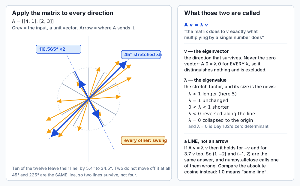
Do that for a lot of arrows — a fan of them, spread evenly all the way around the circle — and you find that this is what happens to almost all of them. They get swung round by five degrees, by twenty degrees, by thirty-four degrees. Each one lands somewhere new.
But not all of them.
For most matrices there are a small number of special directions where the arrow comes back pointing exactly where it started. It is longer, or shorter, or reversed end-for-end. But it is still on its own line. The transformation did not turn it at all; it only scaled it.
That is the whole concept, and here is the sentence to carry away:
Most vectors get knocked off their line when a matrix acts on them. A few do not — they only stretch or squash. Those are the eigenvectors, and how much they stretch is the eigenvalue.
Read that twice. If you can say it to someone else without looking, you have the idea, and everything that follows in this lesson is machinery for finding those directions and knowing what they are good for. The word “eigen” is German for “own” or “characteristic” — an eigenvector is the matrix’s own direction, the one belonging to it, the one it does not disturb.
Here is the measurement, run on a concrete matrix. Take
A = [[4, 1],
     [2, 3]]
and apply it to twenty-four unit vectors, one every fifteen degrees. For each one, record where it pointed, where its output points, and the angle between the two:
   in (deg)   out (deg)   swung by (deg)   length in -> out
   ------------------------------------------------------------
        0      26.565       26.5651        1.000 -> 4.472
       15      33.303       18.3031        1.000 -> 4.933
       30      39.191        9.1914        1.000 -> 5.115
       45      45.000        0.0000        1.000 -> 5.000   <-- kept its direction
       60      51.461        8.5389        1.000 -> 4.600
       75      59.633       15.3674        1.000 -> 3.959
       90      71.565       18.4349        1.000 -> 3.162
      105      91.669       13.3310        1.000 -> 2.381
      120     125.359        5.3590        1.000 -> 1.960
      135     161.565       26.5651        1.000 -> 2.236
      150       4.476       34.4764        1.000 -> 2.973
      165      17.771       32.7711        1.000 -> 3.786
At 45 degrees the swing is zero, and the length went from 1 to exactly 5.
That direction is an eigenvector of A, and 5 is its eigenvalue. No equation
was solved to find it. It was measured.
Now look at the column again, because it has something else to tell you. It does not just dip to zero once. Between 105 and 135 degrees it comes down to 5.36 and climbs back up — which means the true minimum is somewhere between two sample points, and a fan of twenty-four directions stepped straight over it. Sweep every thousandth of a degree instead and a second line appears:
     a surviving line near   45.000000 degrees  (deviation 0.000e+00)
     a surviving line near  116.565000 degrees  (deviation 7.676e-05)
Two lines, not one. That second one is stretched by exactly 2. And the fact that a brute-force sweep can miss an answer is the first argument for having algebra at all — which is what the rest of this lesson builds.
Historical background
The problem is older than the vocabulary by about a century and a half, and it arrived from physics rather than from algebra.
In the 1740s, Jean le Rond d’Alembert was studying a string vibrating between two fixed points, and Leonhard Euler and Joseph-Louis Lagrange were studying systems of coupled oscillators — pendulums linked by springs, that sort of thing. What they kept running into was this: a general motion of such a system looks hopelessly complicated, but there exist particular modes in which the whole system moves together at a single frequency, and every possible motion turns out to be a mixture of those modes. Finding the modes meant solving a polynomial equation whose degree matched the number of parts. That polynomial is the characteristic equation, discovered as a physical question about frequencies long before anyone described it as a matrix problem.
Augustin-Louis Cauchy did the decisive work in the 1820s. Studying the principal axes of quadric surfaces — the natural axes of an ellipsoid, the directions along which it is simply stretched — he proved that a symmetric matrix always has real eigenvalues, which is the result this lesson cites later and which makes principal component analysis behave. Cauchy also introduced the term équation caractéristique, the characteristic equation, and it is his formulation that survives in textbooks today.
The name we use came later still. David Hilbert, working on integral equations around 1904, used the German Eigenwert — literally “own value” or “proper value” — and Eigenvektor alongside it. The half-translated form “eigenvalue” entered English gradually and had not fully displaced the older “proper value” and “characteristic value” until the 1930s. You will still meet “characteristic polynomial” and “spectrum” in the same paragraph as “eigenvalue”; they are historical layers, not distinctions.
Two more dates matter for anyone who intends to compute these things.
Karl Pearson published principal component analysis in 1901, in a paper titled “On Lines and Planes of Closest Fit to Systems of Points in Space”. Harold Hotelling developed it independently and named it in 1933. Pearson’s formulation is worth knowing because it is not the one usually taught: he asked for the line that minimises the total squared perpendicular distance to a cloud of points, which is a different question from ordinary least-squares regression and gives a different answer. That the line he wanted turns out to be the top eigenvector of the covariance matrix is the connection this lesson builds in its own way.
And the QR algorithm, which is what actually runs when you call
numpy.linalg.eig, was published independently by John G. F. Francis in
1961 and Vera Kublanovskaya in 1961–62. It is genuinely one of the great
algorithms of the twentieth century, and it does not compute the characteristic
polynomial at all. That is worth pausing on: the equation every course opens
with is a fine way for a human to solve a 2x2 by hand and a terrible way for a
computer to solve anything larger, because finding polynomial roots is
numerically unstable in a way that finding eigenvalues need not be. The
handwritten method and the library method are two different algorithms that
agree on the answer.
What it is — and what it is not
Let us make the plain-language sentence precise.
A vector v is an eigenvector of a square matrix A if
A v = λ vfor some number λ, and v is not the zero vector. The number λ is the
eigenvalue belonging to v.
Read the equation aloud in words, because the words are the whole point: the
matrix does to v exactly what multiplying by a single number does. The left
side is a matrix-vector product, a genuine transformation with all the machinery
Day 101 built. The right side is a scalar multiplication, which cannot turn
anything — it can only lengthen, shorten, or flip. Saying the two are equal for
this particular v is saying that on this one direction, the transformation has
collapsed into a mere scaling.
Why the zero vector is excluded
This looks like bookkeeping and it is not. Put v = 0 into the equation:
A @ (0, 0) = (0, 0)and λ * (0, 0) = (0, 0) for every value of λ — for 5, for 2, for 1000,
for π. The zero vector satisfies the defining equation for every number there
is, which means it distinguishes nothing, which means it tells you nothing. It
also has no direction to keep, so the question “did it stay on its line?” has no
content. Allowing it would make every number an eigenvalue of every matrix and
the concept would be empty. It is excluded so that the definition says something.
Note the asymmetry: the eigenvalue is allowed to be zero, and the eigenvector is not. An eigenvalue of zero is highly informative — it says the matrix squashes that whole direction down to the origin.
What an eigenvalue tells you
The eigenvalue is a scale factor, and its value carries the news:
| Eigenvalue | What happens to that direction | Example from Day 102 |
|---|---|---|
λ > 1 | Stretched. The longer the arrow, the further it goes each application. | A’s 45-degree line, stretched ×5 |
λ = 1 | Completely unchanged. A fixed direction with a fixed length. | The x-axis under a shear |
0 < λ < 1 | Shortened, but still pointing the same way. | The y-axis under diag(3, 0.5), ×0.5 |
λ = 0 | Collapsed to the origin. That direction ceases to exist. | The y-axis under a projection |
λ < 0 | Reversed. Same line, opposite end. | The y-axis under a reflection, ×−1 |
That λ = 0 row is Day 102 arriving in new clothing. A matrix with a zero
eigenvalue squashes some direction to nothing, which is precisely what a matrix
with determinant zero does. They are the same news reported twice, and this
lesson will make the connection exact.
What it is not
Three misreadings are worth naming, because each one is common and each one produces confident wrong answers.
It is not a vector — it is a line. This is the single most important
correction in this lesson and the one that costs people the most time. If
A v = λ v, multiply both sides by any non-zero number c:
A (c v) = c (A v) = c (λ v) = λ (c v)So c v is an eigenvector too — for every c, including -1 and including
0.001. There is no such thing as the eigenvector for an eigenvalue. There is
an eigen-line through the origin, every point of which except the origin
itself works. A library that hands you one vector has made an arbitrary choice
on your behalf, usually “the unit-length one, with whichever sign fell out of
the routine”. numpy.allclose will therefore call a correct answer wrong,
roughly half the time.
Measured on the authoring machine, for the λ = 2 line of this lesson’s matrix:
       lambda = 2
         mine   [ 0.447214, -0.894427]
         numpy  [-0.447214,  0.894427]
         numpy.allclose(mine, theirs)      -> False
         abs_cosine(mine, theirs)          -> 1.000000000000000
Exact negatives. Both correct. The comparison is the bug, not the answer. The
fix is to compare directions — the absolute cosine of the angle between
them, where 1.0 means “same line” — and never components.
It is not the same as “the biggest number in the matrix”, or the diagonal.
For a diagonal matrix the eigenvalues are the diagonal entries, which makes
diagonal matrices a bad place to build intuition. For [[4, 1], [2, 3]] the
diagonal entries are 4 and 3 and the eigenvalues are 5 and 2. They are not
close, and there is no shortcut.
It is not guaranteed to exist over the real numbers. Some matrices have no real eigenvector at all, and the example is one you can picture perfectly: a rotation of the plane. This is not an edge case, it is one of the most common matrices there is, and the next sections treat it properly rather than apologetically.
Why it was created and what problems it solves
The reason this concept exists — the reason it kept being rediscovered by people studying strings, ellipsoids and integral equations — is that it turns a hard problem into an easy one by changing what you measure things against.
A matrix, in general, mixes your coordinates together. Apply it and the x
component of the answer depends on both x and y of the input. Apply it again
and everything is tangled with everything. Ask what happens after a hundred
applications and you are looking at a hundred matrix multiplications with no
pattern to exploit.
Now suppose you write your starting vector not in terms of x and y, but as a
mixture of the eigenvectors. Something changes completely. The matrix no
longer mixes the ingredients, because an eigenvector is by definition an
ingredient the matrix does not mix — it just scales it. So:
    v0 = c1 * (1, 1)  +  c2 * (1, -2)

    A^k v0 = c1 * 5^k * (1, 1)  +  c2 * 2^k * (1, -2)
A hundred applications is now 5^100 and 2^100, two numbers, computed
directly. The tangle is gone — not because the matrix got simpler but because
you stopped using the wrong coordinates to describe it.
That is what diagonalisation means, and it deserves its plain-language sentence too:
Diagonalisation is changing to the basis where the matrix is just a scaling.
Written out, A = V D V⁻¹, where the columns of V are the eigenvectors and
D is the diagonal matrix of eigenvalues. Read right to left, as Day 101 taught
you to read a product of transformations: V⁻¹ translates your vector into
eigenvector coordinates, D scales each coordinate independently, V translates
back. The complicated matrix in the middle became a list of numbers.
That is the mathematical payoff. Four practical ones follow from it.
Finding structure in data. If your matrix is a covariance matrix, its eigenvectors are the directions your data actually varies along, and its eigenvalues are how much variance sits along each. Sorting the eigenvalues and keeping the large ones is dimensionality reduction, and it is the whole of PCA.
Ranking. If your matrix describes a random walk on a graph — from this page, where do you go next — the dominant eigenvector is the long-run distribution of where the walker spends its time. That is PageRank, and it is why the power method in this lesson is not a toy.
Stability. If a system evolves by repeatedly applying a matrix, the largest eigenvalue magnitude — the spectral radius — decides whether it grows without bound, settles to zero, or holds steady. Above 1 and it explodes; below 1 and it dies away. That single number is the answer to “will this simulation blow up”.
Conditioning. The ratio of the largest to the smallest eigenvalue magnitude tells you how much a small error in your input can be amplified in your output. That is why “ill-conditioned” is a phrase you will meet the first time an inversion gives you nonsense.
How it works
Now the machinery. Everything here is derived from the geometry you have already seen, and nothing is asserted without a reason.
Deriving the characteristic equation
Start with the definition and rearrange it so one side is zero:
    A v = λ v
    A v - λ v = 0
You cannot factor out v yet, because A is a matrix and λ is a number, and
subtracting a number from a matrix is not defined. So write λ as a matrix that
does what multiplying by λ does — the number spread down the diagonal, which is
λI:
(A - λI) v = 0Now read that as a sentence. (A - λI) is one ordinary matrix. It sends the
non-zero vector v to the origin.
Day 102 told you exactly which matrices do that. A matrix that sends a non-zero vector to the origin is one that squashes the plane onto a line or onto a point — it destroys a dimension — and those are precisely the matrices with determinant zero. So:
det(A - λI) = 0There it is. Not asserted, derived, and every symbol in it now stands for
something you have a picture of. It says: find the numbers λ that make
A - λI a squashing matrix, because those are the numbers for which a whole
line survives being sent to the origin.
Solving it for a 2x2
Write A as [[a, b], [c, d]] and expand once:
    A - λI = [[a - λ,      b],
              [    c,  d - λ]]

    det    = (a - λ)(d - λ) - b*c
           = λ² - (a + d)λ + (ad - bc)
The coefficient of λ is a + d, which is the trace of A. The constant is
ad - bc, which is the determinant. So for any 2x2, with no further work
ever:
λ² - (trace)·λ + (determinant) = 0Derive that once and you never do it again. For our matrix, trace is 4 + 3 = 7
and determinant is 4·3 - 1·2 = 10, so:
    λ² - 7λ + 10 = 0
    (λ - 5)(λ - 2) = 0
    λ = 5  and  λ = 2
The discriminant b² - 4c = 49 - 40 = 9 is positive, and its sign is the whole
character of the matrix:
| Discriminant | Eigenvalues | Geometrically |
|---|---|---|
| Positive | Two distinct real values | Two separate directions survive |
| Zero | One repeated real value | One direction survives, or every direction — the eigenvalue alone cannot say which |
| Negative | No real values; a complex conjugate pair | No direction survives; the matrix turns everything |
Reading off the eigenvectors
Once λ = 5 is known, A - 5I has determinant zero, so it squashes the plane
onto a line, and every vector on the line it squashes to the origin is an
eigenvector. There is a whole line of solutions and you only need to name one
point on it.
    A - 5I = [[-1,  1],
              [ 2, -2]]
The first row says -x + y = 0. Any (x, y) with x = y works, so take
(1, 1). Generally, for a row [p, q], the vector (-q, p) satisfies
p·(-q) + q·(p) = 0 for free.
    A - 2I = [[2, 1],
              [2, 1]]
The first row says 2x + y = 0, so take (1, -2).
Check both on paper with no decimals at all:
    A @ (1,  1) = (4 + 1, 2 + 3) = ( 5,  5) = 5 * (1,  1)   ✓
    A @ (1, -2) = (4 - 2, 2 - 6) = ( 2, -4) = 2 * (1, -2)   ✓
Notice what is not determined here. One equation, two unknowns, a whole line
of answers. (1, 1), (2, 2), (-1, -1) and (0.3, 0.3) are all eigenvectors
for λ = 5. This is the sign-and-scale ambiguity arriving as a consequence of
the method rather than as a rule to memorise.
Day 102’s transformations, one at a time
Every matrix from Day 102, and how many directions each one leaves alone. This is
the table to remember, and every row of it was checked two independent ways in
the lab — by numpy.linalg.eig and by brute-force sweeping 180,000 directions:
| Transformation | Eigenvalues | Eigen-lines | Why, geometrically |
|---|---|---|---|
| Identity | 1, 1 | every direction | It leaves everything alone, so everything qualifies |
| Uniform scale ×2 | 2, 2 | every direction | It stretches all directions equally |
Non-uniform scale diag(3, 0.5) | 3, 0.5 | 2 (the axes) | Each axis is scaled by its own factor |
| Reflection in the x-axis | 1, −1 | 2 (the axes) | The x-axis is fixed; the y-axis is flipped, hence −1 |
Shear [[1,1],[0,1]] | 1, 1 | 1 | It leaves the x-axis alone and tilts everything else |
| Rotation by 90° | +i, −i | 0 | It turns every vector, so nothing keeps its line |
| Projection onto the x-axis | 1, 0 | 1, plus a collapsed direction | It flattens the plane onto a line; det 0 |
Three of those rows deserve argument.
The rotation has no real eigenvector, and you can see why before touching any
algebra. A rotation turns every vector by the same angle. For a vector to keep
its line it would have to be turned by 0 or by 180 degrees. A 90-degree
rotation turns by neither. So nothing survives, and there is nothing for the
algebra to find. The algebra says the same thing in its own vocabulary: trace 0,
determinant 1, so λ² + 1 = 0, and no real number squares to −1. The negative
discriminant is not an error message; it is the algebra reporting the
geometry. NumPy returns [0.+1.j, 0.-1.j], which is the honest answer.
This is where a silent disaster lives. Take .real without checking, and:
       values        = [0.+1.j 0.-1.j]
       values.real   = [0. 0.]   <-- both zero. The answer is gone.
Two eigenvalues of magnitude 1 have been silently reported as 0. No exception, no
warning. The habit that prevents it is one if: check that every imaginary part
is below a tolerance before claiming the result is real.
The shear has one eigen-line, but numpy.linalg.eig returns two columns.
This is not a bug, and it is not two directions:
   eigenvalues: [1. 1.]
       column 0: [ 1.00000000000000000,  0.00000000000000000]
       column 1: [-1.00000000000000000,  0.00000000000000022]
   abs_cosine between them = 1.000000000000000
They are the same line. eig must return a square array, so when there are not
enough distinct directions to fill it, it fills the space anyway. Counting
columns would tell you there are two eigendirections; there is one. The
eigenvalue 1 appears twice as a root of the characteristic equation — its
algebraic multiplicity is 2 — while only one independent direction exists,
so its geometric multiplicity is 1. When those two numbers differ, the matrix
cannot be diagonalised, and the shear is the standard example.
And the failure is silent. Attempting V D V⁻¹ on the shear does not raise:
the eigenvector matrix has determinant 2.2e-16 rather than exactly zero, so
LAPACK inverts it happily, returns entries around 4.5e15, and the
reconstruction comes back as a clean, plausible, completely wrong identity
matrix. The reliable check is the condition number, which is above 1e15
here, not the absence of an exception.
A projection has eigenvalue 0, and that is Day 102’s determinant. For
[[1, 0], [0, 0]] the eigenvalues are 1 and 0, the determinant is 0, and the
y-axis is sent to the origin. Two identities hold on every matrix in that table
and are worth carrying:
    the eigenvalues MULTIPLY to the determinant
    the eigenvalues ADD to the trace
So a zero eigenvalue and a zero determinant are the same fact, and the sum and product give you a free arithmetic check on any 2x2 answer you compute.
Symmetric matrices, and why they are the nice case
A matrix equal to its own transpose is symmetric. Two guarantees follow, both standard results proved in any linear algebra text and cited here rather than proved:
- All its eigenvalues are real. No complex pairs, no rotation case.
- Its eigenvectors are orthogonal — mutually at right angles.
Both were checked in the lab rather than assumed, on a 2x2 and on a 3x3 so the
result is not a small-case accident: numpy.linalg.eigh returned float64
values in ascending order, and the largest deviation of V.T @ V from the
identity was 2.220e-16 and 4.133e-16 respectively.
This matters because a covariance matrix is symmetric by construction — entry
(i, j) and entry (j, i) are the same sum of products written in the other
order. So PCA never has to interpret a complex answer, and its components always
come out perpendicular. The pleasantness of PCA is a direct consequence of that
symmetry.
The power method
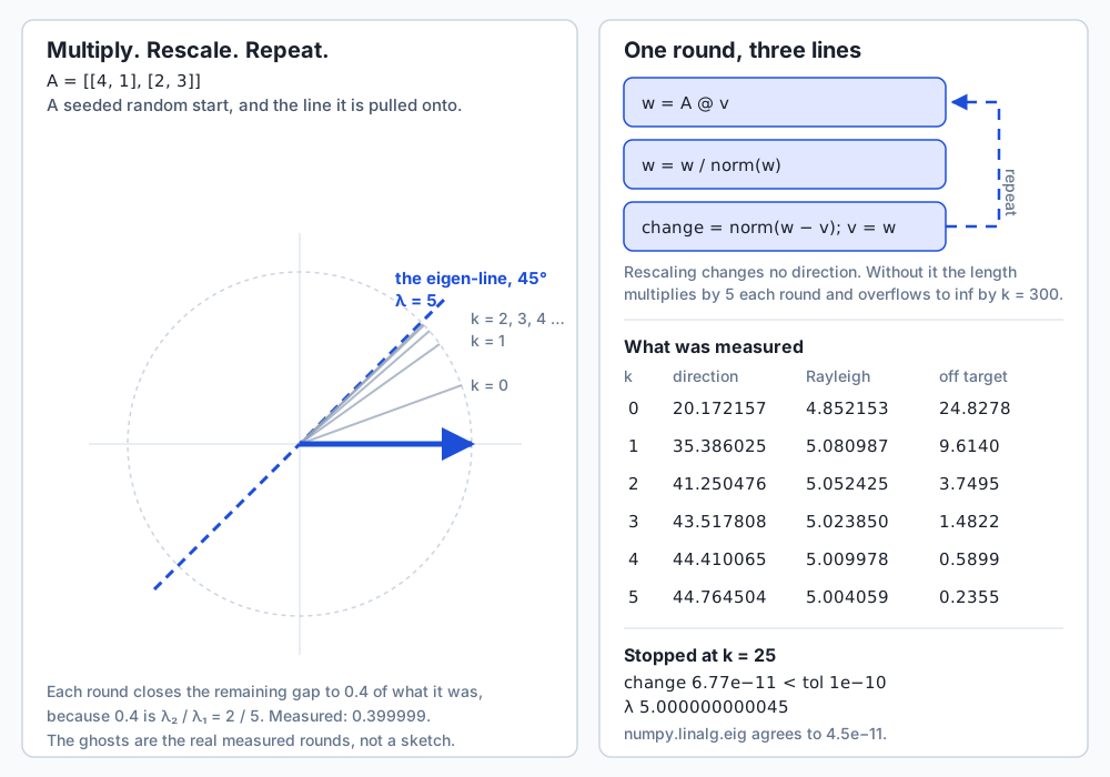
Here is an algorithm for finding the dominant eigenvector that needs no determinant, no polynomial and no library. Multiply by the matrix, rescale to unit length, repeat.
The reason it works is one sentence: write the starting vector as a mixture of the eigenvectors; each application multiplies each ingredient by its own eigenvalue; so the ingredient with the largest-magnitude eigenvalue outgrows all the others, and eventually the mixture is nothing but that direction.
A^k v0 = c1 * 5^k * (1, 1) + c2 * 2^k * (1, -2)The second ingredient shrinks relative to the first by (2/5)^k. After 25
rounds that factor is 1.126e-10 — nothing was eliminated, the dominant
direction simply outgrew the other one. Run from a seeded random start:
    k    direction (deg)   Rayleigh quotient   off target (deg)
    0       20.172157        4.85215311       24.827843
    1       35.386025        5.08098739        9.613975
    2       41.250476        5.05242540        3.749524
    3       43.517808        5.02385040        1.482192
    4       44.410065        5.00997755        0.589935
    5       44.764504        5.00405946        0.235496
   ...
       tolerance          1e-10 on the distance between successive unit vectors
       iterations         25
       eigenvalue         5.000000000045
Two details are not optional and both were measured.
Rescale every round. It changes no direction and costs one division. Without
it the length multiplies by 5 each time, and float64 stops at about 1.8e308:
      k    length of A^k v0
      50    9.304006e+34
     200    6.518845e+139
     300    inf

       after 600 un-normalised rounds:  [inf inf]
       and normalising it now:          [nan nan]
The direction was correct after twenty-five rounds and is now unrecoverable, destroyed by a magnitude nobody asked for.
Align the signs. Negate the new vector when its dot product with the previous one is negative. Without this, a matrix whose dominant eigenvalue is negative flips the iterate end-for-end every single step, so the distance between successive vectors never shrinks and your convergence test never fires — even though the answer settled on round three.
The convergence rate is the eigenvalue ratio, and that is measurable:
      k    change        ratio to previous
      12   1.008750e-05     0.399995
      13   4.034982e-06     0.399998
      14   1.613990e-06     0.399999

   Measured ratio at step 14: 0.399999. Predicted |λ₂/λ₁| = 2/5 = 0.400000.
The algorithm tells you the second eigenvalue through the speed at which it finds the first. Which also tells you exactly when it is a bad idea: eigenvalues of 5 and 4.9 give a ratio of 0.98, and the identical code then needs 962 iterations instead of 25. If the two largest eigenvalues are equal in magnitude it does not converge at all, because there is no single dominant direction to converge to.
One honest note on the Rayleigh quotient, (v · A v) / (v · v), the best
single number to call the eigenvalue for a given v. Textbooks say its error is
the square of the vector’s, so it converges twice as fast. Measured here, that
is true for the symmetric matrix [[2, 1], [1, 2]] — the quotient error divided
by the squared angle locks onto 2.0000 — and false for this lesson’s A,
where the quotient error divided by the angle itself settles on 1.0, merely
linear. The textbook claim carries a condition that is easy to drop: it needs
orthogonal eigenvectors, which symmetry guarantees and A does not have. A’s
two eigen-lines meet at 71.5651 degrees, not 90. The measurement wins over the
remembered rule, and the rule turns out to be right with its condition restored.
An everyday analogy
Take a large sheet of rubber, and print a fine grid on it along with a few dozen arrows radiating out from a dot in the middle. Pin the dot to a board so it cannot move. Now have two people take hold of the edges and pull — not symmetrically, just a good hard uneven pull.
The sheet distorts. The grid squares become parallelograms. Straight lines stay straight, parallel lines stay parallel, and the pinned centre stays put: that is exactly Day 102’s linear transformation, and the rubber sheet is not a decoration, it is a physical model of it.
Now look at your arrows. Almost every one of them is now pointing somewhere else. An arrow that pointed north-east before the pull is pointing more nearly east afterwards, and one that pointed north has swung a bit too. They have been turned, and by different amounts depending on where they started.
But run your eye all the way around, and you find one or two arrows that are still lying along exactly the line they started on. They are longer than they were — noticeably longer, because the sheet stretched most in that direction — but they were not turned at all. Those are the eigenvectors of that pull, and how much longer they got is the eigenvalue.
The analogy carries the rest of the lesson, so let us push it deliberately:
- An arrow that came out shorter but still on its line has an eigenvalue between 0 and 1: the sheet was compressed in that direction.
- An arrow that came out pointing backwards along its line has a negative eigenvalue. The sheet was folded through the centre in that direction.
- An arrow that vanished into the pin — the sheet crushed flat along that line — has eigenvalue zero, and that is exactly the state in which the pull cannot be undone, because you cannot recover which point on that line each crushed point came from. Determinant zero, no inverse, Day 102.
- Pull the sheet uniformly in all directions and every arrow keeps its line, which is the identity and the uniform scaling: every direction is an eigenvector.
- Twist the sheet instead of pulling it and no arrow keeps its line, which is the rotation. There is no eigenvector to find, and the sheet is telling you the truth rather than being difficult.
Two places the analogy is honest about its own limits, which is why it is worth having.
Direction, not arrowhead. An arrow and the same arrow drawn pointing the other way lie on the same line on the sheet, and the pull treats them identically. This is the sign ambiguity, and the sheet makes it feel obvious rather than pedantic: what survives a stretch is a line through the pin, and which end you painted the head on was never part of the physics.
Pull it again and again. Apply the same pull repeatedly. The arrow that grows
by a factor of 5 each time and the arrow that grows by 2 each time start out
comparable and rapidly stop being: after twenty-five pulls the first is
(5/2)^25 — about ten million — times longer relative to the second. Every arrow
on the sheet, whatever it started as, is eventually lying almost exactly along
the fastest-growing direction, simply because everything else has been left
behind. That is the power method, and it is why the dominant eigenvector takes
over.
Where the analogy breaks, and it is worth knowing: rubber has a physical limit and real matrices do not, and a real sheet resists in ways a linear map does not model at all. The analogy is for the geometry of one application, not for the material.
Examples in practice
PCA: the eigenvectors of a covariance matrix
This is the day’s strongest artifact and the connection to make permanent: principal component analysis is the eigenvectors of a covariance matrix, and the largest eigenvalue is the direction of greatest variance.
Build a cloud of 400 points, deliberately stretched along 30 degrees — standard
deviation 3.0 along that direction, 0.4 across it — and centred at (5, −2).
That 30 degrees is written nowhere in the array handed to the code; the
algorithm has 800 coordinates and nothing else.
Step one: centre the data. Subtract the mean of each column. This is the step people skip and it is not optional; the section below shows what it costs.
Step two: compute the covariance matrix, C = (Xᶜᵀ Xᶜ) / (n − 1):
   from scratch:                        numpy.cov(cloud, rowvar=False):
       [ 6.34888382   3.57798121]           [ 6.34888382   3.57798121]
       [ 3.57798121   2.25100160]           [ 3.57798121   2.25100160]
   identical to 1e-12? True
Read the entries: C[0][0] is how much x varies, C[1][1] is how much y
varies, and C[0][1] is how much they vary together — positive here, meaning
points further right also tend to be higher, which is what a cloud tilted upward
at 30 degrees looks like.
Step three: take the eigenvectors. There is no step four.
       numpy.linalg.eigh eigenvalues, sorted large to small:
           [8.42306158, 0.17682384]

       top component      [-0.86514150, -0.50152786]
       its direction      30.101134 degrees
       the truth          30.0 degrees
       error              0.101134 degrees
Found, from 400 pairs of coordinates and nothing else. That is PCA, complete, in about fifteen lines.
The eigenvalues are just as useful. The eigenvalue is the variance along its own eigenvector, so its square root is the standard deviation:
       eigenvalue 1   8.423062   sqrt = 2.902251   (built with sd 3.0)
       eigenvalue 2   0.176824   sqrt = 0.420504   (built with sd 0.4)

       proportion of variance explained: [0.97943881, 0.02056119]
Both recover the numbers the cloud was built with — not exactly, because 400
samples estimate a spread rather than reproduce it. And that
0.9794 is the sentence behind every “we reduced 768 dimensions to 50” claim
you will read: sort the eigenvalues, keep the ones that add up to enough of the
total, discard the rest.
There is one more property that PCA quietly buys you. Project every point onto each component and measure the correlation between the two projections:
       spread along component 1  2.902251
       spread along component 2  0.420504
       correlation between them  6.420e-16
Uncorrelated to within rounding. Not just the best directions, but directions along which your data carries no shared information — which follows directly from the eigenvectors of a symmetric matrix being orthogonal.
The sign trap, sprung where it matters
Look again at that top component: [-0.86514150, -0.50152786], against a true
direction of [0.866025, 0.500000]. They point opposite ways along the same
line. numpy.allclose returns False. The absolute cosine is 0.9999984422.
The answer is exactly right.
A principal component names an axis, not an arrow, and any code that cares which end is which has a bug waiting in it. This is not a curiosity: sign flips between library versions, between BLAS builds, and between runs on different hardware are routine, and a pipeline that branches on the sign of a component will work for a year and then not.
What forgetting to centre costs
       Xᵀ X / (n−1) with NO centring:
       its top eigenvector points at 166.583965 degrees
       the correct answer is           30.0 degrees
       error                          136.583965 degrees

       the cloud's CENTRE lies at 158.198591 degrees from the origin
       distance from the uncentred answer to that:       8.385374 degrees
       distance from the uncentred answer to the truth: 136.583965 degrees
The uncentred answer sits close to the direction of the cloud’s offset from the
origin and nowhere near its shape. That is what the calculation actually
measured, because without centring the squared offset (5² + 2² = 29) swamps the
real spread (8.4). No exception, no warning, a confident wrong answer 136
degrees out. This is the failure mode that matters, and the reason it is worth
building PCA by hand once.
From two dimensions to seven hundred and sixty-eight
Replace the two-column cloud with a matrix of 768-dimensional sentence embeddings and nothing about the method changes. The covariance matrix becomes 768 by 768, its top eigenvectors are the directions those embeddings actually vary along, and the eigenvalues tell you how many of the 768 dimensions carry real information rather than noise. Everything in this lesson scales without modification; only the arithmetic gets bigger.
Implications: security, privacy, performance, scalability, and cost
Performance. numpy.linalg.eig on a general matrix is roughly cubic in the
matrix dimension, so doubling the size multiplies the work by about eight. On a
400 by 400 symmetric float64 matrix, best of five runs on the authoring
machine:
         numpy.linalg.eig            64.79 ms
         numpy.linalg.eigh            6.19 ms
         numpy.linalg.eigvals        17.77 ms
         numpy.linalg.eigvalsh        3.69 ms

       eig / eigh = 10.46x on this run, on this machine.
Four separate lessons in that block, and only one of them is a timing.
eigh beats eig by an order of magnitude because it is solving an easier
problem — symmetry buys real algorithmic structure. Asking only for the values
and not the vectors saves roughly two thirds. And the ratio itself is one
machine on one day: it depends on your BLAS build, your core count and your
thermal state, so nothing in the lab asserts it. What the lab does assert is
that the two routines’ 400 eigenvalues agree to within 1.990e-13.
Scalability. This is where the power method stops looking naive. eig needs
the whole matrix as a dense array and works on all of it. The power method needs
only the ability to compute A @ v. On a web graph with a hundred million nodes
the adjacency matrix does not fit in memory as an array — but multiplying by it
is just a walk over the edges. The method that is obviously inferior for a 2x2 is
the only one that survives at scale, and every serious large-scale eigensolver
(Lanczos, Arnoldi, and scipy.sparse.linalg.eigsh) is a refined descendant of
it.
Cost. Everything in this lesson runs on your own machine with two free
packages. There is no service to call and no meter running. The cost that does
bite is the cubic scaling: an eigendecomposition of a 20,000 by 20,000 dense
matrix is a serious computation and a 200,000 by 200,000 dense one is not
happening at all, which is exactly when you switch to asking for the top k
eigenvalues of a sparse matrix instead of all of them.
Numerical stability. The honest warning of this section. Three silent failures were measured in the lab, and none of them raised anything:
numpy.linalg.eighon a non-symmetric matrix returns a confident wrong answer. It reads one triangle and assumes the other matches, so onAit quietly solves[[4, 2], [2, 3]]instead and returns[1.438, 5.562].numpy.linalg.invon the shear’s singular eigenvector matrix does not raise; it returns entries around4.5e15and a plausible wrong reconstruction.- Forgetting to centre before a covariance gives an answer 136 degrees out.
A repeated or nearly repeated eigenvalue is the general danger zone: when two eigenvalues are close, the individual eigenvectors become extremely sensitive to tiny perturbations even though the subspace they span is perfectly stable. If your eigenvectors jitter between runs on almost identical data, suspect a near- degenerate pair rather than a bug.
Privacy. Nothing in this lesson processes personal data, but PCA is frequently pointed at data that is, and two points deserve stating plainly. First, a principal component is a linear combination of your columns, so if one of them encodes a sensitive attribute the top component can still carry it after you drop that column, because a correlated column reconstructs it. Dimensionality reduction does not anonymise. Second, every row contributes to the covariance matrix, so a covariance matrix derived from personal records is itself derived personal data and inherits the handling rules of the records.
Security. The relevant exposure here is the supply chain and the
deserialisation surface rather than the mathematics. Nothing in this lesson
parses untrusted input. The one habit worth carrying: numpy.load with
allow_pickle=True executes arbitrary code from the file it loads, so it is
never the right default for a matrix you did not write yourself.
Alternatives: free, open source, and commercial
Everything in this area is free and open source. There is no paid eigensolver worth naming for this work, and that is genuinely unusual — the entire ecosystem sits on LAPACK, which has been public since 1992.
I ran two of the following. numpy.linalg.eig and numpy.linalg.eigh were
run on numpy 2.5.2 on the authoring machine and every figure quoted for them in
this lesson is from a real run. The rest are described from their own
documentation, are not installed here, and no output from any of them is
reproduced anywhere in this day.
numpy.linalg.eig — ran it
When to choose it: any square matrix, when you need both values and vectors and cannot promise symmetry. It is the general-purpose default.
How to use it:
values, vectors = np.linalg.eig(A)
top = int(np.argmax(np.abs(values)))       # eig promises NO ordering
Concrete example: on [[4, 1], [2, 3]] it returns [5.+0.j, 2.+0.j] and the
matching unit eigenvectors as columns of a complex128 array.
Two things to know before you rely on it. It returns complex128 even when
every eigenvalue is real — measured on numpy 2.5.2 for A, for numpy.eye(2),
for numpy.diag([1., 2., 3.]) and for an integer matrix — which contradicts its
own docstring, quoted exactly:
“The resulting array will be of complex type, unless the imaginary part is zero in which case it will be cast to a real type.”
The imaginary part is zero and the cast does not happen. When documentation
and measurement disagree, the measurement wins; this lesson records what it
observed on one machine on one day, and if a future version starts casting, the
lab’s test for this will go red and that is the correct outcome. The practical
consequence: values.astype(float) emits a ComplexWarning, and the fix is
values.real — guarded by a check that the imaginary parts really are
negligible, because on a rotation that same line silently destroys the answer.
And it promises no ordering whatsoever, so “the largest eigenvalue” needs an
argmax, never an index.
Free vs paid: free and open source, BSD 3-Clause. No account, no key.
numpy.linalg.eigh — ran it
When to choose it: whenever the input is symmetric (or Hermitian). Covariance matrices, Gram matrices, graph Laplacians, correlation matrices — always.
How to use it:
variances, directions = np.linalg.eigh(covariance)   # ascending order
order = np.argsort(variances)[::-1]                  # largest first for PCA
Concrete example: on [[2, 1], [1, 2]] it returns [1., 3.] as float64,
already sorted ascending, with orthogonal eigenvectors.
Three concrete advantages, all measured: float64 rather than complex128, so
no .real and no guard; values returned sorted ascending, which eig never
promises; and roughly ten times faster on a 400 by 400 on this machine. The
catch, and it is a sharp one: eigh reads only one triangle of the input and
assumes the other matches. Hand it a non-symmetric matrix and it does not
complain — it answers a question about a different matrix. Check symmetry, or
know for structural reasons that it holds.
Companion routines numpy.linalg.eigvals and numpy.linalg.eigvalsh return
values only, at roughly a third of the cost, when you do not need the vectors.
scipy.linalg.eig / eigh — not run here
The same jobs with more control: the generalized problem A v = λ B v, the
option to request only a range of eigenvalues rather than all of them, and an
explicit choice of LAPACK driver. Reach for it when NumPy’s version does not take
the argument you need. Free and open source, BSD 3-Clause.
scipy.sparse.linalg.eigs / eigsh — not run here
For matrices too large to hold densely. You ask for the k largest or smallest
eigenvalues rather than all of them, and it needs only the ability to multiply by
the matrix — the same requirement the power method has, which is not a
coincidence: these are industrial-grade relatives of it, built on the Lanczos and
Arnoldi iterations. This is what you use for a graph with millions of nodes, and
eigsh is the symmetric variant. Free and open source, BSD 3-Clause.
torch.linalg.eig / eigh — not run here
The same interface on tensors, so it runs on a GPU and participates in automatic differentiation. Choose it when the eigendecomposition sits inside a model being trained rather than beside it as an analysis step. Free and open source, BSD-style.
sklearn.decomposition.PCA — not run here
PCA as a fitted object, with the centring, the sorting, the explained-variance
ratios and a transform method handled for you — and with a singular value
decomposition underneath rather than an explicit covariance matrix, which is
numerically more accurate on ill-conditioned data because it never forms XᵀX
and never squares your condition number. Use it for real work. The fifteen
lines in this lesson exist so you know what it is doing and why the sign
sometimes flips. Free and open source, BSD 3-Clause.
Comparison with related concepts
| Concept | What it gives you | How it relates to today |
|---|---|---|
| Determinant (Day 102) | One number: the area scale factor | The product of the eigenvalues. Zero determinant ⟺ some eigenvalue is zero ⟺ a direction was collapsed |
| Trace | The sum of the diagonal | The sum of the eigenvalues. Together with the determinant it is the characteristic equation for a 2x2 |
| Rank | How many dimensions survive | For a diagonalisable matrix, the number of non-zero eigenvalues |
| Singular values (SVD) | How much the matrix stretches in each of its own input/output directions | Always real and non-negative, and defined for non-square matrices too. For a symmetric positive-definite matrix they coincide with the eigenvalues; in general they do not |
| Eigenvalues | How much each surviving direction is scaled | Today. Only defined for square matrices, and may be complex |
| Diagonalisation | A = V D V⁻¹ | The eigen-decomposition written as a factorisation. Fails exactly when there are too few independent eigenvectors — the shear |
| Spectral radius | The largest eigenvalue magnitude | Decides whether repeated application grows or decays. What the power method converges towards |
The SVD versus eigenvalues distinction is the one worth internalising,
because it is where people most often reach for the wrong tool. Eigenvalues need
a square matrix and can be complex; singular values are defined for any matrix
of any shape and are always real and non-negative. Your data matrix is n rows
by d columns and is almost never square, so it has singular values but no
eigenvalues. Its covariance matrix is d by d, symmetric, and has both — and
the singular values of the centred data matrix are the square roots of the
eigenvalues of that covariance matrix, times a constant. That relationship is why
scikit-learn’s PCA can use an SVD to answer an eigenvalue question, and do it
more accurately.
The other comparison worth stating: algebraic versus geometric multiplicity. The algebraic multiplicity of an eigenvalue is how many times it appears as a root of the characteristic equation; the geometric multiplicity is how many independent eigenvectors it actually has. Geometric is never greater than algebraic. When they are equal for every eigenvalue, the matrix diagonalises; when they differ, it does not. The shear — algebraic 2, geometric 1 — is the canonical example and the reason the concept has two names.
When to use it — and when not to
Use an eigendecomposition when:
- You want the directions your data varies along most. That is PCA, and the matrix to decompose is the covariance matrix.
- You want the steady state of a repeated process — a random walk on a graph, a Markov chain, an iterated map. The dominant eigenvector is where it settles.
- You need to know whether a repeated process grows or decays. Compare the spectral radius against 1; nothing else is needed.
- You are applying the same matrix many times and want a closed form.
Diagonalise once and the
k-th application is a list ofk-th powers. - Your matrix is symmetric. Everything is well behaved: real values, orthogonal vectors, a fast dedicated routine.
Do not reach for it when:
- Your matrix is not square. Eigenvalues are not defined. Use the SVD.
- You want the principal components of a data matrix and accuracy matters.
Forming
XᵀXsquares the condition number; take the SVD of the centred data instead, which is what scikit-learn does. - You only need to solve
A x = b. Use a solver. Computing an eigendecomposition to solve a linear system is enormously more work for a worse answer. - Your matrix is large and sparse and you want all the eigenvalues. You
probably do not want all of them; ask for the top
kwith a sparse iterative method. - The eigenvalues you care about are close together. The individual eigenvectors will be numerically unstable even though the subspace they span is fine, and the power method in particular will crawl — 962 iterations at a ratio of 0.98 against 25 at 0.4.
- Your matrix is defective — too few independent eigenvectors, like the shear. Diagonalisation does not exist, and worse, the attempt fails silently. Check the condition number of the eigenvector matrix.
Use the power method specifically when the matrix is too large to hold
densely but you can multiply by it, and you only need the dominant eigenpair. Do
not use it when you need all of them, when the top two eigenvalues are close in
magnitude, or when the matrix is small — for a 2x2 there is no reason on earth
not to call eig.
Knowledge check
Eight questions in quiz.yml, including one on why a plane rotation has no real
eigenvectors and one on the sign-and-scale ambiguity. Before you take it, try to
answer these three from memory, because they are the ones that matter:
- State in one sentence what an eigenvector and an eigenvalue are, without using the words “characteristic”, “determinant” or “polynomial”.
- Why does a 90-degree rotation of the plane have no real eigenvector? Answer from the geometry first, then say what the algebra reports and why the two are the same statement.
- Your code computes an eigenvector and gets
[0.447, -0.894]. The reference answer is[-0.447, 0.894].numpy.allclosesaysFalse. What is wrong, and what should you have compared instead?
Hands-on exercise
The lab is “The Vectors That Keep Their Direction”. Five exercises: write six functions, then make twenty-six predictions and let the tests check them.
cd labs/sections/math-statistics-and-data/day-106-eigenvalues-and-eigenvectors-intuitively
python3 -m venv .venv
.venv/bin/pip install -r requirements/requirements.txt
.venv/bin/pytest starter -q
Then work through starter/00_brief.md:
- Six functions in
starter/eigen.py— the absolute cosine, the characteristic coefficients, the 2x2 eigenvalues, an eigenvector from a real eigenvalue, the power method, and a covariance matrix from scratch. - Solve the 2x2 by hand and record trace, determinant, discriminant, both eigenvalues and both eigenvectors.
- Predict what each of Day 102’s transformations does to directions —
including how many eigen-lines a shear has, and what dtype
eigreturns. - Predict the power method’s behaviour — which eigenvalue, which direction, what convergence ratio, and what un-normalised iteration does.
- Build the PCA and predict where the top component points, whether
numpy.allclosewill agree with it, and what skipping the centring costs.
Then read the six reference scripts in examples/, which print the whole story
with real numbers.
Expected output
On an untouched checkout:
1 passed, 52 skippedWhen you have finished, 53 passed. The full harness ends with:
110 checks, 0 failure(s).Values you should reproduce exactly:
   Directions that came back on their own line: [45, 225]
     a surviving line near   45.000000 degrees  (deviation 0.000e+00)
     a surviving line near  116.565000 degrees  (deviation 7.676e-05)

   eigenvalues  = [5.+0.j 2.+0.j]
   dtype        = complex128

       iterations         25
       eigenvalue         5.000000000045

       top component      [-0.86514150, -0.50152786]
       its direction      30.101134 degrees
       the truth          30.0 degrees
Validate your work
bash tests/run_tests.sh; echo "exit=$?"Expect 110 checks, 0 failure(s). and exit=0. Check the script’s own status,
never a pipeline’s — bash tests/run_tests.sh | tail -3; echo $? reports
tail’s status, not the harness’s.
Section 6 of the harness re-runs the whole suite with one expectation deliberately swapped for the naive belief that a shear has two eigendirections, and asserts that the re-run names the failure and exits non-zero. A green test suite proves nothing until you have watched it go red.
Troubleshooting
numpy.sqrt returned nan on the rotation. A rotation’s discriminant is
negative. numpy.sqrt(-4.0) is nan with a warning; numpy.emath.sqrt(-4.0) is
2j, which is the answer. This is the difference between “no real eigenvalues,
and here is why” and “something went wrong”.
The power method never converges. Almost always the missing sign alignment,
and it only shows up when the dominant eigenvalue is negative. On
numpy.diag([-5.0, 2.0]) the iterate flips end-for-end every step, so the
distance between successive vectors stays at 2.0 forever even though the
direction settled on round one. Negate w when numpy.dot(w, v) < 0.
pytest starter still says 52 skipped after you wrote code. Run it from the
lab directory, not from inside starter/; remove the return NotImplemented
line; and set the value in answers.py rather than only computing it.
Your covariance is close to NumPy’s but not equal. You divided by n instead
of n − 1. If it is wildly out, you forgot to subtract the mean.
troubleshooting.md in the lab covers the full list, including a table of
results that look wrong and are not.
Common mistakes
Comparing eigenvectors component by component. The mistake that costs the most time, because the code looks right and the answer is right. Compare absolute cosines. Do not “fix” a sign — you will make one case pass and another fail.
Counting eig’s columns as eigendirections. It returns a square array
because it must. The shear’s two columns lie on one line, absolute cosine 1.0.
Count lines.
Taking .real without checking. On a rotation this silently reports two
eigenvalues of magnitude 1 as 0. Guard it with a check on the imaginary parts.
Handing a non-symmetric matrix to eigh. No error, no warning, an answer
about a different matrix.
Skipping the centring in PCA. 136 degrees wrong, confidently.
Believing the Rayleigh quotient always converges quadratically. It needs orthogonal eigenvectors. On this lesson’s non-symmetric matrix it converges merely linearly, measured.
Practice assignment
Do these without looking at the lab’s reference solutions.
-
Work a fresh 2x2 by hand, end to end. Take
B = [[3, 1], [1, 3]]. Compute trace, determinant, discriminant, both eigenvalues, and an eigenvector for each. VerifyA v = λ vwith integer arithmetic and no decimals. Then check the sum against the trace and the product against the determinant — that is a free correctness check on any answer you produce, and you should be doing it every time. -
Predict, then measure, for three new matrices. For each of
[[2, 0], [0, 2]],[[0, 1], [1, 0]]and[[1, 2], [0, 1]]: how many eigen-lines does it have, and what are the eigenvalues? Answer from the geometry first — what does each one do to the plane? — then check againstnumpy.linalg.eig. The second one is a reflection in the 45-degree line, and it is worth working out which direction gets the negative eigenvalue before you run anything. -
Demonstrate the sign ambiguity to yourself deliberately. Take any matrix, get its eigenvectors from
numpy.linalg.eig, negate one column, and verify thatA v = λ vstill holds exactly. Then write the two-line comparison function that gets this right, and use it from now on. -
Time the convergence rate. Run the power method on matrices with eigenvalue ratios of 0.2, 0.4, 0.8 and 0.95 — for example
numpy.diag([5, 1]),numpy.diag([5, 2]),numpy.diag([5, 4])andnumpy.diag([5, 4.75]). Record the iteration count for each at a tolerance of1e-10and plot or tabulate it against the ratio. You should see the count blow up as the ratio approaches 1, and you should be able to explain why from the mixture argument rather than from the graph. -
PCA on something of your own. Take any table with three or four numeric columns. Standardise each column to zero mean and unit variance first, then compute the covariance matrix and take its eigenvectors with
eigh. Read the top component as a set of weights: which columns does it lean on? Write one honest paragraph interpreting it — and note what would have happened had you not standardised, when one column is measured in thousands and another in fractions.
Extension challenge
Four, in rough order of difficulty. All of them are checkable against
numpy.linalg.eig or eigh, and you should check.
1. The inverse power method — find the smallest eigenvalue. Run the power
method on numpy.linalg.inv(A) instead of A. Before you do, prove to yourself
why it works: if A v = λ v with λ ≠ 0, then multiplying both sides by
A⁻¹/λ gives A⁻¹ v = (1/λ) v. Inverting a matrix inverts its eigenvalues and
leaves its eigenvectors exactly where they were, so the dominant eigenvector of
the inverse is the least dominant eigenvector of A. Verify that claim on
paper first, then use it. This is a real technique with a real name.
2. Deflation. Once you have the dominant eigenpair (λ₁, v₁) of a symmetric
matrix with v₁ normalised, subtract λ₁ * numpy.outer(v₁, v₁) from it and run
the power method again. You should get the second eigenvector. Try it on the
lab’s SYMMETRIC_3X3 and check all three against numpy.linalg.eigh. Then try it
on the non-symmetric A and work out why it does not work there — the answer
is orthogonality, and finding it yourself is the exercise.
3. Break the power method on purpose. Build a matrix whose two eigenvalues
have the same magnitude but opposite signs, such as numpy.diag([3.0, -3.0]).
Predict what the iteration does, write the prediction down, then run it. There is
no single dominant direction, and the honest outcome is that it never converges.
Then answer the harder question: what does the sequence of iterates do, and can
you describe it exactly?
4. Complex eigenvectors are real objects. numpy.linalg.eig on a rotation
returns complex eigenvectors as well as complex eigenvalues, and this lesson
has so far treated them only as a signal that no real answer exists. Verify that
A v = λ v still holds exactly for those complex pairs. Then work out what the
real and imaginary parts of a complex eigenvector mean geometrically: together
they span the plane in which the rotation is happening, and the eigenvalue’s
argument is the angle. For a 2x2 rotation this is the whole plane and the fact is
uninteresting; do it for a 3x3 rotation about an axis and it becomes very
interesting indeed, because the real eigenvector you also get back is the axis
of rotation itself.
The AI thread
Here is the honest version of why this day exists.
You will almost never write an eigensolver. You will call
sklearn.decomposition.PCA or torch.linalg.eigh and get a correct answer in
one line. What today buys you is not the ability to compute; it is the ability to
interpret, and to recognise when the one-line answer is not the one you wanted.
Three concrete situations, all of which you will meet.
You reduce 768-dimensional embeddings to 50 and someone asks why 50. The answer is in the eigenvalues: sort them, take the running total, and find where the curve flattens. That number is not a hyperparameter you tune by validation score — it is a property of your data that you can read off directly, and being able to say “the top 50 carry 94% of the variance and the next 50 carry 3%” is a different quality of answer than “50 worked”.
Your clustering results change when you standardise your columns, and you do not know whether that is a bug. It is not. Covariance is not scale-invariant, so a column measured in thousands dominates the top eigenvector purely by unit choice. Whether you standardise is a modelling decision about what “variation” should mean for your problem, and today is what lets you see that it is a decision at all rather than a step you either remembered or forgot.
A pipeline that has worked for a year starts producing mirrored results after a library upgrade. An eigenvector is defined up to sign, the library changed which sign it returns, and any downstream code that branched on that sign is now wrong. This is not hypothetical; it is one of the most common reproducibility failures in applied machine learning, and it is invisible unless you know that a component names an axis rather than an arrow.
Underneath all three is one idea that the rest of this course keeps returning to. A matrix is a transformation, transformations mix your coordinates together, and an eigenvector is a direction where the mixing stops. Finding those directions is finding the coordinates in which your problem was simple all along. Attention weights, covariance structure, graph connectivity, the stability of a training run — these are different problems wearing the same mathematics, and the sentence you learned at the top of this lesson is the key to all of them:
Most vectors get knocked off their line. A few do not. Those are the eigenvectors, and how much they stretch is the eigenvalue.
Quiz
Q1. You apply a matrix to twenty-four unit vectors spread evenly around the circle and record the angle between each input and its output. Twenty-two of the angles are non-zero. What are the two directions where the angle came out as zero?
- Eigenvectors of the matrix, and the factor by which each one changed length is its eigenvalue
- The columns of the matrix, which is where the basis vectors land
- The directions in which the determinant is largest
- Artefacts of sampling — with a finer fan those angles would be non-zero too
Show answer
Answer: A. Eigenvectors of the matrix, and the factor by which each one changed length is its eigenvalue
That measurement IS the definition. A vector whose output lies on the same line as its input has been scaled but not turned, which is exactly what A v = lambda v says: the matrix did to v precisely what multiplying by a single number does. The length ratio is lambda. The second option confuses today with Day 102: the columns of a matrix are where the basis vectors (1, 0) and (0, 1) land, which is a fact about the matrix but tells you nothing about which directions survive — for the matrix [[4, 1], [2, 3]] the columns are (4, 2) and (1, 3) while the eigen-lines sit at 45 and 116.565 degrees. The third option is not a thing: a determinant is one number for the whole matrix, not something that varies by direction. The fourth gets it backwards — a coarser fan MISSES eigendirections rather than inventing them, which is exactly what happened in the lesson: the twenty-four-direction fan found the 45-degree line and stepped straight over the one at 116.565 degrees, which only a 180,000-direction sweep recovered.
Q2. Why is the zero vector excluded from the definition of an eigenvector, even though A 0 = lambda 0 is a true equation?
- Because the zero vector cannot be normalised to unit length
- Because it satisfies the equation for every value of lambda, so it distinguishes nothing
- Because matrix multiplication is undefined for the zero vector
- Because its eigenvalue would have to be zero, and zero is not allowed as an eigenvalue
Show answer
Answer: B. Because it satisfies the equation for every value of lambda, so it distinguishes nothing
A @ (0, 0) is (0, 0), and lambda * (0, 0) is also (0, 0) — for lambda = 5, for lambda = 2, for lambda = 1000, for every number there is. So the zero vector satisfies the defining equation universally, which means it separates no eigenvalue from any other and carries no information. Allowing it would make every number an eigenvalue of every matrix and empty the concept out completely. It also has no direction to keep, so the question the definition is really asking — did this direction survive? — has no content for it. The first option is true but is a consequence rather than the reason; plenty of useful objects cannot be normalised. The third is simply false: A @ 0 is perfectly well defined and equals 0. The fourth inverts the actual rule, and the inversion matters: the EIGENVALUE is allowed to be zero and the EIGENVECTOR is not. An eigenvalue of zero is highly informative — it says the matrix collapsed that entire direction to the origin, which is the same news as a zero determinant.
Q3. Why does a 90-degree rotation of the plane have no real eigenvector?
- Because its determinant is 1, and only matrices with determinant 0 have eigenvectors
- Because rotation matrices are not square, so eigenvalues are undefined for them
- Because it turns every vector by 90 degrees, so no vector can come back on its own line
- Because numpy.linalg.eig fails to converge on rotation matrices
Show answer
Answer: C. Because it turns every vector by 90 degrees, so no vector can come back on its own line
Answer it from the geometry and the algebra becomes a footnote. A rotation turns EVERY vector by the same angle. For a vector to keep its line it would have to be turned by 0 degrees or by 180 degrees, and a 90-degree rotation turns by neither — so nothing survives, and there is nothing for any algebra to find. The lesson confirmed this by measurement as well: over 180,000 swept directions the smallest swing was 90.000000 degrees, and the sweep returned the verdict none. The algebra then says the same thing in its own vocabulary: trace 0 and determinant 1 give lambda squared plus 1 = 0, and no real number squares to minus 1. The negative discriminant is not an error message, it is the algebra reporting the geometry. The first option has the relationship backwards — a zero determinant means some eigenvalue is zero, not that eigenvectors exist only then; the identity has determinant 1 and every direction is an eigenvector of it. The second is false: a rotation matrix is square. The fourth is false and worth being clear about — eig succeeds perfectly well and returns 0+1j and 0-1j, which is the honest answer rather than a failure. The real danger here is taking .real without checking, which silently reports two eigenvalues of magnitude 1 as 0.
Q4. Your hand calculation gives the eigenvector (0.447, -0.894). numpy.linalg.eig returns (-0.447, 0.894) for the same eigenvalue, and numpy.allclose says False. What is going on?
- NumPy uses a different sign convention that you should convert to before comparing
- One of the two answers is wrong, and the residual of A v minus lambda v will show which
- Both are correct — an eigenvector is defined only up to sign and scale, so comparing components is the bug
- The tolerance in allclose is too tight for this calculation and should be relaxed
Show answer
Answer: C. Both are correct — an eigenvector is defined only up to sign and scale, so comparing components is the bug
If A v = lambda v, multiply both sides by any non-zero number c and you get A (c v) = lambda (c v). So c v is an eigenvector too, for every c — including minus 1 and including 3.7. There is no such thing as THE eigenvector for an eigenvalue; there is an eigen-LINE through the origin, and every library that hands you a single vector has made an arbitrary choice on your behalf. Which sign LAPACK returns is a detail of its internal normalisation, not a fact about your matrix, and it can differ between builds and between versions. The fix is to compare directions with the absolute cosine, where 1.0 means same line. The first option is a trap worth naming because it sounds professional: there is no convention to convert to, because there is nothing to convert — attempting to normalise the sign yourself makes one case pass and another fail, and you end up back here in an hour. The second is wrong: BOTH residuals are zero, because both vectors genuinely satisfy the equation. The fourth misdiagnoses entirely — the two answers differ by a factor of exactly minus 1, not by a rounding error, so no tolerance short of 2.0 would help and relaxing it would only hide real failures.
Q5. The shear [[1, 1], [0, 1]] has eigenvalues 1 and 1, and numpy.linalg.eig returns a 2x2 array of eigenvectors. How many distinct eigendirections does it actually have?
- Two, one per column returned
- Zero, because the repeated eigenvalue means the decomposition failed
- One — both returned columns lie on the same line, and their absolute cosine is 1.0
- Infinitely many, because a repeated eigenvalue always means every direction qualifies
Show answer
Answer: C. One — both returned columns lie on the same line, and their absolute cosine is 1.0
The measured absolute cosine between the two returned columns is 1.000000000000000: they are the same line. eig must return a square array, so when there are not enough independent directions to fill it, it fills the space anyway — which means counting columns is not counting eigendirections. Geometrically it is obvious: a shear leaves the x-axis alone and tilts everything else, so only the horizontal line survives, and a brute-force sweep of 180,000 directions independently found exactly one. The eigenvalue 1 appears twice as a root of the characteristic equation, so its ALGEBRAIC multiplicity is 2, while only one independent direction exists, so its GEOMETRIC multiplicity is 1. That gap is precisely what makes the shear impossible to diagonalise, and the failure is silent: numpy.linalg.inv on its singular eigenvector matrix does not raise — the determinant is 2.2e-16 rather than exactly 0, so LAPACK inverts it, returns entries around 4.5e15, and V D V-inverse comes back as a clean, plausible, completely wrong identity matrix. Check the condition number, not for an exception. The fourth option describes the identity and the uniform scaling, where a repeated eigenvalue DOES come with every direction qualifying — so a repeated eigenvalue alone cannot tell you which case you are in.
Q6. You run the power method on a matrix with eigenvalues 5 and 2, and it converges in 25 iterations. You then run the identical code on a matrix with eigenvalues 5 and 4.9. What happens, and why?
- It converges in about the same number of iterations, since the dominant eigenvalue is unchanged
- It needs far more iterations — 962 in the lab — because the error shrinks by the ratio of the two eigenvalues each round
- It converges faster, because the two eigenvalues are closer so less separation is needed
- It fails immediately, because the power method requires distinct integer eigenvalues
Show answer
Answer: B. It needs far more iterations — 962 in the lab — because the error shrinks by the ratio of the two eigenvalues each round
Write the starting vector as a mixture of the eigenvectors. Each application of the matrix multiplies each ingredient by its own eigenvalue, so after k rounds the second ingredient has shrunk RELATIVE to the first by (lambda 2 over lambda 1) to the power k. Nothing is eliminated — the dominant direction simply outgrows the other one, and the speed at which it does so is entirely governed by that ratio. For 2 over 5 the ratio is 0.4, measured in the lab at 0.399999, and 25 rounds suffice for a tolerance of 1e-10. For 4.9 over 5 the ratio is 0.98, and the same code needed 962 iterations. This is why the algorithm effectively tells you the second eigenvalue through the speed at which it finds the first, and it is the honest answer to when NOT to use the power method. The third option inverts the mechanism: closeness in magnitude is exactly what makes the dominant direction hard to isolate, because the competing ingredient refuses to die away. The fourth is false — the method has no integer requirement at all and works on any matrix with a single dominant eigenvalue. What genuinely breaks it is two eigenvalues of EQUAL magnitude, such as 3 and minus 3, where there is no single dominant direction to converge to and the iteration never settles.
Q7. You compute PCA on a cloud of points by taking the eigenvectors of X-transpose X divided by n minus 1, but you forget to subtract the column means first. The cloud is genuinely elongated along 30 degrees. What do you get?
- The correct 30 degrees, since centring only shifts the data and eigenvectors ignore shifts
- An exception, because a covariance matrix is undefined for uncentred data
- A result rotated by exactly 90 degrees from the truth
- A confident answer around 166.6 degrees, roughly 136.6 degrees wrong, with no error or warning
Show answer
Answer: D. A confident answer around 166.6 degrees, roughly 136.6 degrees wrong, with no error or warning
The measured result was 166.583965 degrees against a truth of 30.0, an error of 136.583965 degrees, and nothing was raised. Covariance is about how points vary AROUND THEIR OWN MEAN. Skip the subtraction and every product picks up the offset of the cloud from the origin, which for this cloud is (5, minus 2) and describes where it sits rather than what shape it is. The numbers make the mechanism plain: the squared offset is 5 squared plus 2 squared = 29, while the actual spread contributes about 8.4, so the offset simply swamps the signal. Confirming the diagnosis, the uncentred answer lands 8.385374 degrees from the direction of the cloud CENTRE and 136.583965 degrees from its shape — it measured the offset, faithfully. The first option is a plausible-sounding half-truth: eigenvectors are indeed unaffected by scaling the whole matrix, which is why dividing by n versus n minus 1 does not matter, but they are absolutely affected by which matrix you built. The second is wrong and is the heart of why this is dangerous — no library checks, because X-transpose X is a perfectly well-formed matrix and there is no way for it to know you meant something else. The third invents a structure that is not there; the error depends entirely on where your cloud happens to sit relative to the origin.
Q8. You have a covariance matrix and you need its eigenvectors. Why is numpy.linalg.eigh the right call rather than numpy.linalg.eig?
- Because a covariance matrix is symmetric by construction, and eigh returns real sorted values, is much faster, and is written for exactly that case
- Because eig cannot handle matrices larger than 2 by 2
- Because eigh normalises the eigenvectors to unit length and eig does not
- Because eigh is guaranteed to return components with a positive first entry, which removes the sign ambiguity
Show answer
Answer: A. Because a covariance matrix is symmetric by construction, and eigh returns real sorted values, is much faster, and is written for exactly that case
Entry (i, j) and entry (j, i) of a covariance matrix are the same sum of products written in the other order, so symmetry is structural rather than something you hope for — and symmetry guarantees real eigenvalues and orthogonal eigenvectors, which is why PCA is so well behaved. eigh is the routine written for that case and it pays three measured dividends: it returns float64 rather than complex128, so no .real and no guard against a rotation-style disaster; it returns values sorted ascending, whereas eig makes no ordering promise at all and needs an argmax; and on a 400 by 400 symmetric matrix on the authoring machine it took 6.19 ms against 64.79 ms, a factor of 10.46 on that run. The sharp edge to know about is the other direction: eigh reads only ONE triangle of the input and assumes the other matches, so handed a non-symmetric matrix it does not complain — on [[4, 1], [2, 3]] it silently solves [[4, 2], [2, 3]] and returns 1.438 and 5.562 instead of 2 and 5. The second option is simply false. The third is false too — both routines return unit-length eigenvectors. The fourth is the tempting one and it is wrong: eigh fixes nothing about the sign, which is exactly why the lesson PCA result came back as (minus 0.865, minus 0.502) against a true direction of (0.866, 0.500), pointing the opposite way along the identical line while being exactly correct.
Glossary
- Eigenvector
- A non-zero vector that a matrix scales but does not turn: applying the matrix leaves it on exactly the line it started on, only longer, shorter, or reversed. Formally, v is an eigenvector of A if A v = lambda v for some number lambda, with v not the zero vector. The critical subtlety is that it is really a LINE rather than a vector: if A v = lambda v then the same equation holds for minus v and for 3.7 v, so every non-zero multiple is equally an eigenvector. Any library that returns one vector has made an arbitrary choice, which is why comparing eigenvectors component by component is a bug and comparing absolute cosines is not. The word is half-translated German: eigen means own or characteristic, so this is the matrix own direction.
- Eigenvalue
- The scale factor belonging to an eigenvector — how much the matrix stretches that direction. Its value is the news: above 1 means stretched, exactly 1 means unchanged, between 0 and 1 means shortened, negative means reversed end-for-end along the same line, and exactly 0 means the direction was collapsed to the origin. That last case is Day 102 zero determinant arriving in new clothing. Note the asymmetry with its partner: an eigenVALUE of zero is permitted and highly informative, while an eigenVECTOR of zero is excluded because it satisfies the defining equation for every lambda and therefore distinguishes nothing.
- Characteristic equation
- The polynomial equation det(A minus lambda I) = 0, whose roots are the eigenvalues. It is not an arbitrary formula but a direct translation of the geometry: rearranging A v = lambda v gives (A minus lambda I) v = 0, which says a non-zero vector is sent to the origin, and only a matrix with zero determinant does that. For any 2x2 it always works out to lambda squared minus (trace) lambda plus (determinant) = 0, so trace and determinant are the only two numbers you need. Derive that once and never again. Its DISCRIMINANT carries the whole character of the matrix: positive means two distinct real eigenvalues, zero means one repeated, negative means none that are real. Worth knowing that no serious numerical library computes it — the QR algorithm finds eigenvalues without ever forming the polynomial, because polynomial root-finding is unstable in a way that eigenvalue-finding need not be.
- Dominant eigenvalue
- The eigenvalue of largest absolute value, and the eigenvector belonging to it is the dominant eigenvector. It matters because repeated application of a matrix is eventually governed by it alone: writing any starting vector as a mixture of the eigenvectors, each application multiplies each ingredient by its own eigenvalue, so the ingredient with the largest magnitude outgrows every other one. Nothing is eliminated; it is simply left behind. Note that dominant is about MAGNITUDE, so minus 5 dominates 2. When two eigenvalues share the largest magnitude there is no dominant direction at all, and iterative methods that assume one will never converge.
- Power method
- An algorithm for finding the dominant eigenvector in three lines: multiply by the matrix, rescale to unit length, repeat until successive vectors stop moving. Rescaling changes no direction and exists only to stop the length running away — without it the vector grows by the eigenvalue every round and overflows float64 to infinity within a few hundred steps, destroying a direction that was already correct. Sign alignment is equally non-optional: when the dominant eigenvalue is negative the iterate flips end-for-end every step, so the convergence test never fires even though the answer settled on round three. Its convergence RATE is the ratio of the second eigenvalue to the first, measured at 0.399999 for a matrix with eigenvalues 5 and 2. It looks naive next to numpy.linalg.eig, and it is, for a small matrix — but it needs only the ability to compute A times v rather than the matrix itself, which is why every large-scale eigensolver is a refined descendant of it.
- Diagonalisation
- Rewriting a matrix as A = V D V-inverse, where the columns of V are the eigenvectors and D is the diagonal matrix of eigenvalues. In one sentence: changing to the basis where the matrix is just a scaling. Read right to left as Day 101 taught, V-inverse translates a vector into eigenvector coordinates, D scales each coordinate independently, and V translates back — so the complicated matrix in the middle has become a list of numbers, and the k-th application becomes a list of k-th powers. It is possible exactly when there are enough independent eigenvectors to fill V. When there are not — as for a shear — the matrix is called DEFECTIVE and diagonalisation does not exist. The dangerous part is that the attempt fails silently: numpy.linalg.inv on a singular eigenvector matrix does not raise, it returns entries around 4.5e15 and a plausible wrong answer.
- Symmetric matrix
- A square matrix equal to its own transpose, so entry (i, j) always matches entry (j, i). Two guarantees follow, both standard results proved in any linear algebra text and cited rather than proved in this lesson: all its eigenvalues are REAL, and its eigenvectors are ORTHOGONAL. Cauchy proved the real-eigenvalue result in the 1820s while studying the principal axes of quadric surfaces. This is not a niche case — a covariance matrix, a Gram matrix, a correlation matrix and a graph Laplacian are all symmetric by construction, which is precisely why PCA never returns a complex answer you have to interpret and why its components always come out perpendicular. It is also why numpy.linalg.eigh exists and is roughly ten times faster than eig on such input.
- Orthogonal
- At right angles — two vectors are orthogonal when their dot product is zero, which Day 103 established means a cosine similarity of zero and no shared component at all. For a set of vectors it means every pair is mutually perpendicular. Symmetry of a matrix guarantees its eigenvectors are orthogonal, which is what gives PCA its second useful property beyond finding the best directions: the projections of the data onto different principal components are UNCORRELATED, measured at 6.420e-16 in this lesson. It is also the hidden condition on the textbook claim that the Rayleigh quotient converges quadratically — measured, that holds for a symmetric matrix and fails for a non-symmetric one whose eigen-lines meet at 71.5651 degrees rather than 90.
- Covariance matrix
- For data with d features, the d by d matrix whose (i, j) entry is how much feature i and feature j vary TOGETHER around their own means. Computed as the centred data transposed times itself, divided by n minus 1. Two things about it decide everything downstream. It is always symmetric, because entry (i, j) and entry (j, i) are the same sum of products written in the other order — which is what guarantees real eigenvalues and perpendicular eigenvectors. And the CENTRING is not optional: skip it and you measure how far the cloud sits from the origin rather than how it is shaped, which in this lesson produced an answer 136.583965 degrees wrong with no error and no warning. Note that its size depends on the number of FEATURES, not the number of points: a 400 by 2 dataset has a 2 by 2 covariance matrix.
- Principal component
- An eigenvector of a covariance matrix. The FIRST principal component is the one with the largest eigenvalue, and it is the direction along which the data varies most; each subsequent one is the direction of greatest remaining variance perpendicular to all the earlier ones. Principal component analysis is nothing more than computing these and keeping the ones whose eigenvalues are large — in this lesson the top component of a 400-point cloud came back at 30.101134 degrees against a true elongation of 30.0 that the code was never told. The eigenvalue IS the variance along its own component, so its square root is a standard deviation, and the proportions of the total are the explained-variance ratios behind every claim that 768 dimensions were reduced to 50. Because a component is an eigenvector it names an AXIS rather than an arrow: sign flips between library versions are routine and are not errors. Published by Karl Pearson in 1901 and independently named by Harold Hotelling in 1933.
- Spectral radius
- The largest absolute value among a matrix eigenvalues. The word spectrum for the set of eigenvalues comes from Hilbert work on integral equations, predating its use in physics for what a prism does to light. The spectral radius is the single number that answers whether repeated application of a matrix grows or decays: above 1 and the iterates grow without bound, below 1 and they shrink to nothing, exactly 1 and they hold steady. That makes it the honest one-number stability test for anything driven by an iterated linear map, and it is what the power method converges towards. Related and worth knowing alongside it: the ratio of largest to smallest eigenvalue magnitude is the CONDITION NUMBER, which measures how much a small error in the input can be amplified in the output.
- Multiplicity
- How many times an eigenvalue counts, in two different senses that can disagree. ALGEBRAIC multiplicity is how many times it appears as a root of the characteristic equation. GEOMETRIC multiplicity is how many independent eigenvectors it actually has. Geometric is never greater than algebraic, and when they are equal for every eigenvalue the matrix diagonalises. The shear [[1, 1], [0, 1]] is the canonical example of them disagreeing: its eigenvalue 1 has algebraic multiplicity 2 and geometric multiplicity 1, because only the x-axis survives. This matters practically because numpy.linalg.eig must return a square array of eigenvectors regardless, so it returns two columns for the shear whose absolute cosine is 1.0 — the same line twice. Counting the columns a library returns is not counting eigendirections.
Sources and further reading
- NumPy documentation — NumPy Developers (accessed 2026-08-17)
- Eigenvalues and eigenvectors — Wikipedia (accessed 2026-08-17)
- Transformation matrix — Wikipedia (accessed 2026-08-17)
- Matrix (mathematics) — Wikipedia (accessed 2026-08-17)
- Essence of linear algebra — 3Blue1Brown (accessed 2026-08-17)
- Linear Algebra, Spring 2010 (18.06) — MIT OpenCourseWare (accessed 2026-08-17)
Kept in this browser, no account needed. Your progress page turns the whole record into one link you can bookmark or open on another device.