Math, Statistics, and Data › Linear Algebra II and Calculus › Day 109
Day 109: Partial Derivatives and Gradients

After this lesson you will know which way is uphill, and you will have proved it rather than been told it. You will be able to say what a partial derivative is in one sentence — one input moves, everything else is held still — and compute one by hand and numerically for a function of two variables and a function of three. You will assemble those partials into a gradient and read its two halves separately: its direction is the way uphill, its length is how steep, and it has one component per INPUT rather than one per dimension of the graph. Then you will demonstrate the two facts everyone asserts and almost nobody shows. You will measure the rate of change along 360 separate bearings, each with its own direct central difference that never forms a gradient, and watch the winner land on the gradient's own bearing to within the half-degree the sampling grid allows — with the winning rate divided by the gradient's length equal to the cosine of that gap to nine decimal places. And you will show the gradient is perpendicular to the contour without cheating: every contour is an exact algebraic curve derived from the function alone and checked to hold f constant before it is used, because rotating a gradient ninety degrees and calling the result a contour direction proves nothing. You will learn what a zero gradient does not tell you — minimum, maximum and saddle are indistinguishable from it — and why saddles dominate in high dimensions. You will carry Day 108's U-shaped error curve into two dimensions, watch a cubic's truncation error come out as exactly h squared, and find the trough at 1e-5 for a central difference and 1e-8 for a forward one, both landing where the cube root and square root of machine epsilon predict. You will meet the honest limit that a plane's constant gradient becomes unmeasurable when the function's values are large, with the roundoff bound tracking the damage across seven orders of magnitude. And you will finish holding the number that explains autodiff: a numerical gradient costs two evaluations of the whole function per parameter, which is two million forward passes to take one training step on a million-parameter model.
Hands-on lab for this lesson
Lab files on GitHub: https://github.com/ai-roadmap-365/ai-roadmap-365.github.io/tree/main/labs/sections/math-statistics-and-data/day-109-partial-derivatives-and-gradients
- Get the hands-on files. Clone the labs repository once (you can reuse this clone for every lesson). This works on macOS, Linux, and Windows (PowerShell or WSL):
git clone https://github.com/ai-roadmap-365/ai-roadmap-365.github.io.git cd ai-roadmap-365.github.io - Open this lesson's lab. Move into the directory for this specific day. Every lab lives at the same predictable path — section / subsection / week / day:
cd labs/sections/math-statistics-and-data/day-109-partial-derivatives-and-gradients - Read the lab guide. Open `README.md` in that directory. It lists the exact commands, what each does, the expected output, and how to check your work — read it before running anything.
- Run it and check your work. Follow the README's "How to run" section: run the example first to see the finished result, then complete the numbered exercises in `starter/`, then run the tests. The tests pass (exit 0) only when your work is correct.
bash tests/run_tests.sh # or the test command named in the lab README
You can also open the lab as a local page (works offline, shows the file tree and expected output).
Learning objectives
By the end of this lesson you will be able to:
- Define a partial derivative as the ordinary derivative with every other input held constant, and say what the rounded d announces
- Compute partial derivatives by hand for a quadratic, a plane, a product and a cubic, then verify each one numerically with a central difference
- Build a gradient as the vector of partial derivatives, for a function of two inputs and of three, and explain why it has one component per input rather than one per dimension of the graph
- Read a gradient's direction and its length as answers to two different questions, with different units
- Compute a directional derivative two ways — as a dot product with the gradient, and by measuring directly along the bearing — and use their agreement as evidence
- Demonstrate that no direction climbs faster than the gradient by sweeping 360 bearings, and derive the result from the geometric dot product
- Demonstrate that the gradient is perpendicular to the contour using an exactly parametrised curve, and explain why rotating the gradient would prove nothing
- Define a contour and a level set, and say why every optimisation picture in this course is drawn with them
- Identify a stationary point, and state plainly that a zero gradient cannot distinguish a minimum from a maximum from a saddle
- Explain why saddle points dominate stationary points in high-dimensional parameter spaces
- Choose a step size deliberately, predict the h-squared truncation law, and locate the trough of the error curve for both a central and a forward difference
- Recognise where a numerical gradient stops being trustworthy, and predict the damage with the roundoff bound eps times the size of f over 2h
- Distinguish numpy.gradient, which differences a sampled array, from a gradient of a callable function, and name the edge_order default that catches people
- Count the cost of a numerical gradient as two evaluations per parameter, and state precisely what reverse-mode automatic differentiation changes about that
- Name the Jacobian and the Hessian, say what each one is, and say which question each answers that the gradient cannot
Prerequisites
- Day 108 — derivatives, the central difference, and the U-shaped error curve. Today is that plus four words: and hold everything else still
- Day 99 — vectors, length and unit vectors. A gradient is a vector and every property from that day still applies
- Day 103 — the dot product and its geometric reading as length times length times cosine. That reading is the entire proof of steepest ascent
- Day 104 — NumPy arrays, linspace and elementwise arithmetic; the lab uses NumPy to hold results, never to differentiate anything
- Day 70 — floating point, which is why one whole section of this lesson is about subtracting two nearly equal numbers
- Day 43 — python3 -m venv and installing a package with pip; the lab installs numpy and pytest into a lab-local environment
- Days 71 to 74 — pytest, which the lab uses for both the reference suite and the running score
- No school calculus is assumed anywhere, and none is used
Why this matters
You are standing on a hillside. Someone asks you how steep it is.
Yesterday that question had an answer. A curve has one slope at each point, you measure it by nudging the input a little and seeing what the output does, and the number you get is the derivative. Day 108 did that carefully: the shrinking interval, the tangent, the central difference, and the U-shaped error curve where making h too small makes the answer worse rather than better.
On a hillside the question breaks.
Walk north and the ground climbs steeply. Walk east and it barely rises. Walk north-east and you get something in between. Walk along the side of the hill at just the right angle and you stay perfectly level. There is no single number called “the slope here”, because there is no single direction to walk in — and the moment a function has two inputs instead of one, that is the situation you are in.
This matters more than it sounds, because every function you will ever want to optimise has more than one input. A model’s loss depends on all of its parameters at once. Not one weight — every weight, simultaneously. A network with a million parameters is a landscape in a million-dimensional space, and “which way is downhill from here” is the only question training ever asks.
Today’s answer has two halves, and both of them are things you can compute before you finish reading.
The first half is the partial derivative, and it is a piece of bookkeeping rather than a new idea. Freeze every input but one. A function of two variables with one of them frozen is a function of one variable, and you already know how to differentiate one of those. Do it once per input. That is all a partial derivative is, and by the end of the next section you will have computed two of them by hand.
The second half is the part that earns a new name. Collect those partial derivatives into a vector — Day 99’s kind of vector, with a length and a direction — and the resulting object does something that none of the individual partials do. It points in the direction of steepest increase, and its length is how steep that is. That is the sentence the next three days are built on. Day 110 shows how to compute it efficiently through composed functions, Day 111 turns “step against it” into an algorithm, and Day 112 draws the pictures.
So it had better be true, and it had better be demonstrated rather than asserted. Almost every introduction to gradients states the steepest-ascent property as though it were obvious, and it is not obvious at all: it says that two numbers measured along the axes somehow know about every direction in between. Today’s lab measures the rate of change along 360 separate bearings, one per degree, each one with its own direct measurement that never forms a gradient — and finds that the winner is the gradient’s bearing, every time.
There is a second fact that gets asserted even more casually, and it is the one that makes the pictures in the rest of this course readable: the gradient is perpendicular to the contour line through the point. A contour is a line of constant height, the thing on a walking map that tells you where the cliffs are. Perpendicular to it is the only direction with anything to gain. The lab checks this too, and it checks it carefully, because the lazy way to demonstrate it is circular — rotate the gradient by ninety degrees, call the result the contour direction, and marvel at the right angle you built.
The cost of getting this wrong is not abstract. If you cannot tell a gradient from a partial derivative you will misread every optimiser’s documentation. If you believe a zero gradient means you have found the answer, you will stop training at a saddle point and never know why the loss plateaued. And if you think the numerical differentiation you write today is how models are actually trained, you will not understand why automatic differentiation exists — a question the closing section of this lesson answers with arithmetic rather than adjectives.
The idea in plain language
Here is the whole day in one paragraph, before any notation at all.
A function of several inputs is a landscape. Standing anywhere on it, you can ask “if I change only this one input, and hold everything else absolutely still, what happens to the output?” That question has a single number for an answer, and that number is a partial derivative. Ask it once per input. Line up the answers. The list you get is the gradient, and it is not just a list — it is a vector, so it has a direction and a length, and both of them mean something. The direction is the way uphill. The length is how steep the ground is that way.
Now with a function you can hold in your head.
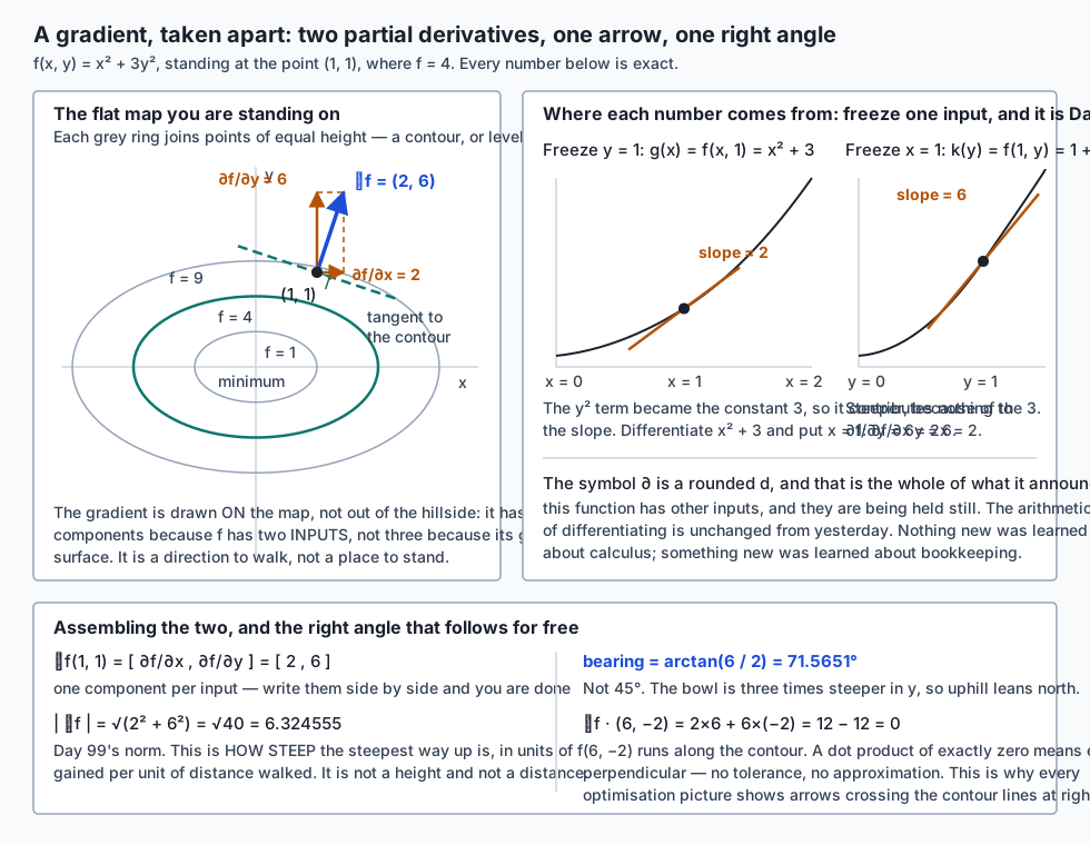
f(x, y) = x² + 3y²This is a bowl. Its lowest point is at the origin, where f is zero, and it climbs as you move away in any direction. It is not a round bowl: the 3 in front of y² makes it three times steeper in y than in x at the same distance out. Think of a valley that is narrow across and gentle along.
Stand at the point (2, 1), where f = 2² + 3(1²) = 7.
Freeze y at 1. What is left is a function of x alone:
g(x) = f(x, 1) = x² + 3That 3 is not a variable any more. y is frozen at 1, so 3y² is frozen at 3, and a frozen thing contributes nothing to a rate of change. Differentiate x² + 3 the way Day 108 taught you — the derivative of x² is 2x, the derivative of a constant is zero — and put x = 2:
dg/dx = 2x = 4 (at x = 2)Now freeze x at 2 instead. What is left is a function of y alone:
k(y) = f(2, y) = 4 + 3y²Differentiate and put y = 1:
dk/dy = 6y = 6 (at y = 1)Those two numbers, 4 and 6, are the partial derivatives of f at (2, 1). They say: from here, one step east gains about 4 units of height per unit of distance, and one step north gains about 6.
The notation writes them with a rounded d instead of a straight one:
∂f/∂x = 4 ∂f/∂y = 6and the rounded ∂ announces exactly one thing: this function has other inputs, and they are being held still. That is the entire meaning of the symbol. The arithmetic of differentiating is unchanged from yesterday. Nothing new was learned about calculus; something new was learned about bookkeeping.
Collect the two into a vector and write it with the nabla symbol ∇, an upside-down triangle, pronounced “del”:
∇f(2, 1) = [ ∂f/∂x , ∂f/∂y ] = [4, 6]And that object — two numbers in square brackets — is a Day 99 vector. It has a length, √(4² + 6²) = √52 ≈ 7.2111, and it has a direction, a bearing of about 56.31° from due east. The claim of the day is that if you stand at (2, 1) and walk along that bearing, f increases faster than along any other bearing you could have chosen, and it increases at 7.2111 units of f per unit of distance walked.
Historical background
The notation came before the idea was settled, which is unusual and worth a moment.
The symbol ∂ is not a Greek letter and not a rounded d by accident. Wikipedia’s article on the partial derivative records that “one of the first known uses of this symbol in mathematics is by Marquis de Condorcet from 1770”, who used it for partial differences rather than derivatives. The modern usage came later: “the modern partial derivative notation was created by Adrien-Marie Legendre (1786), although he later abandoned it; Carl Gustav Jacob Jacobi reintroduced the symbol in 1841.”
Two things in that sentence are worth noticing. The first is the gap: seventy-one years between Condorcet’s first use and Jacobi’s reintroduction, and fifty-five between Legendre inventing the modern form and abandoning it and Jacobi bringing it back. Notation that now looks inevitable took the better part of a century to stick. The second is why it needed to stick at all. As long as you are differentiating a function of one variable, df/dx is unambiguous. The moment there are several variables, df/dx no longer says what is happening to the others — and in some fields the answer genuinely varies. Wikipedia notes that in areas like statistical mechanics “it may be necessary to specify explicitly which variables are being held constant to avoid ambiguity”, and the convention there is to write the held-constant variables as subscripts outside a bracket. The rounded ∂ is a compressed version of that warning: something is being held still; make sure you know what.
The ∇ symbol has a different flavour of history, and this lesson will not reach for dates it cannot check. What the cited sources do state plainly is what it is: “the nabla symbol ∇, written as an upside-down triangle and pronounced ‘del’, denotes the vector differential operator”. It is an operator, not a number — it is a thing that eats a function and produces a vector field.
The more interesting historical point is not about symbols at all. It is that for most of the two hundred and fifty years these symbols have existed, gradients were computed by hand, symbolically. You wrote down the function, you differentiated it with a pencil, you got a formula, and you evaluated the formula. That is still the fastest and most accurate route when the function is small enough to write down.
What changed is scale. A modern model’s loss is a function you cannot write down in any useful sense — it is millions of arithmetic operations composed together — and its gradient has one component per parameter. Differentiating that by hand is not merely tedious; it is not a thing a person does. The two responses to that problem are the subject of this lesson’s alternatives section: numerical differentiation, which is what you will build today and which is honest but expensive, and automatic differentiation, which is what every training loop in the world actually uses.
The lesson’s own contribution to this history is small and worth stating: this course teaches the expensive method first, on purpose, because you cannot appreciate what autodiff bought you until you have counted what it replaced.
What it is — and what it is not
A partial derivative is the ordinary derivative of a function of one variable, obtained by freezing all the other variables. Wikipedia’s definition is exactly this: “a partial derivative of a function of several variables is its derivative with respect to one of those variables, with the others held constant”.
A partial derivative is not a different kind of derivative with its own rules. Every rule from Day 108 applies unchanged. The ∂ is a note to the reader, not an instruction to the mathematics.
A gradient is the vector whose components are the partial derivatives, one per input. Wikipedia states its defining property in a way that is worth reading twice: “the gradient of f is defined as the unique vector field whose dot product with any unit vector v at each point x is the directional derivative of f along v.” That is a definition, not a theorem — the gradient is defined as the thing that makes the dot product come out right. Everything else follows from it.
A gradient is not a point on the surface, and it is not a number. This is the single most common misreading, so it deserves the space. Take f(x, y) = x² + 3y². Its input has two coordinates. Its output is one number. Its graph is a surface sitting in three dimensions. The gradient has two components, not three. It is an arrow drawn on the flat map you are standing on, pointing in the direction you should walk. It is not an arrow pointing up out of the hillside. If you ever find yourself with a three-component gradient for a two-input function, you have made this mistake.
A gradient is not guaranteed to point uphill for every function that has partial derivatives. This is the caveat that most introductions leave out, and the cited source is unusually clear about it. Wikipedia gives the example of
f(x, y) = (x² · y) / (x² + y²)(defined to be 0 at the origin), which “is not differentiable at the origin as it does not have a well defined tangent plane despite having well defined partial derivatives in every direction at the origin”, and notes that there “the above formula for gradient fails to transform like a vector … and also fails to point towards the ‘steepest ascent’ in some orientations”. The steepest-ascent property needs the function to be differentiable, which is a stronger condition than “the partial derivatives exist”. Every function in today’s lab is a polynomial and is differentiable everywhere, so the property holds throughout — but it is a property with a condition on it, and “the partials exist” is not that condition.
A zero gradient is not a minimum. It is a stationary point, which Wikipedia names as such: “a point where the gradient is the zero vector is known as a stationary point”. It might be a minimum, a maximum, or a saddle, and the gradient contains no information whatsoever about which. The section below on how it works demonstrates all three with identical gradients.
numpy.gradient is not what you build today. It is a good function doing a different job, and the comparison is instructive enough that the lab devotes a section to it.
Here is the whole vocabulary in one place.
| Term | What it is | Shape, for a function of n inputs |
|---|---|---|
Partial derivative ∂f/∂xᵢ | Rate of change of f when input i moves and the rest are frozen | one number |
Gradient ∇f | The vector of all n partial derivatives | a vector of n numbers |
|∇f| | How steep the steepest ascent is, per unit distance | one number |
Directional derivative ∇f · u | Rate of change along a chosen unit direction u | one number |
| Contour / level set | The set of points where f takes one fixed value | a curve when n = 2, a surface when n = 3 |
| Stationary point | A point where ∇f is the zero vector | a location, not a number |
| Jacobian | The matrix of partials when f returns a vector, one row per output | m × n matrix |
| Hessian | The matrix of second partials of a scalar f | n × n matrix |
The last two are named here and developed no further. The Jacobian is what a gradient becomes when the function has several outputs rather than one — Day 110’s chain rule is the reason it matters. The Hessian is the object that would tell you whether a stationary point is a minimum, a maximum or a saddle, and it is the reason the gradient cannot.
Why it was created and what problems it solves
The partial derivative solves a bookkeeping problem: how do you talk about a rate of change when there is more than one thing that could be changing? The answer — say which one, and freeze the rest — is so simple that it barely feels like an invention. It is, though, and the fifty-five-year gap between Legendre’s notation and Jacobi’s reinstatement of it suggests the field took a while to agree it was needed.
The gradient solves a much sharper problem, and it is worth being precise about what it is.
Suppose you have a function of two inputs and you want to know the rate of change along some direction — not along an axis, but along a diagonal, a bearing of 37° say. One route is to measure it: step a small distance along that bearing, step the same distance back, and divide the change by the total distance moved. That is just Day 108’s central difference with the step taken along a diagonal instead of along an axis, and it works perfectly.
But it answers one question. Ask about 38° and you have to measure again. Ask about all 360 whole-degree bearings and you have made 720 evaluations of f.
The gradient is a compression. Two numbers, computed once at a cost of four evaluations, answer the question for every direction simultaneously, through the dot product:
D_u f = ∇f · uThat is the thing worth appreciating. It is not that the gradient gives you the steepest direction — that is a consequence. It is that the gradient is a complete summary of the function’s first-order behaviour at that point, from which the rate along any bearing whatsoever can be recovered with a dot product, and Day 103 already taught you what a dot product costs.
The steepest-ascent property falls straight out of that compression, and here is the argument in full, because it takes three lines and most treatments skip it. Day 103 gave the geometric reading of the dot product:
a · b = |a| |b| cos θApply it with a = ∇f and b = u, remembering that u is a unit vector so |u| = 1:
D_u f = ∇f · u = |∇f| cos θwhere θ is the angle between your chosen direction and the gradient. Now |∇f| is a fixed number — it does not depend on which direction you picked. The only thing that varies is cos θ, and cosine has a maximum value of exactly 1, attained when θ = 0, which is to say when u points along the gradient. So:
- the largest possible rate of change is
|∇f|, achieved by walking along∇f; - the smallest (most negative) is
−|∇f|, achieved by walking exactly the opposite way — which is gradient descent, and the whole of Day 111; - a rate of zero happens when
cos θ = 0, that is whenθ = 90°, which is to say perpendicular to the gradient — and a direction along whichfdoes not change is, by definition, a direction along the contour.
That last bullet is the perpendicularity result, and notice that it did not need a separate argument. Wikipedia puts it the same way: “the dot product (∇f)ₓ · v of the gradient at a point x with a vector v gives the directional derivative of f at x in the direction v. It follows that in this case the gradient of f is orthogonal to the level sets of f.”
The same source offers a concrete version that is worth carrying around. Suppose the steepest slope on a hill is 40%. A road going straight up has a 40% gradient. A road at 60° from the uphill direction has a slope of “40% times the cosine of 60°, or 20%”. You can check that in your head, and it is the entire theory.
How it works
Computing a partial derivative numerically
A computer cannot read x² + 3y² and differentiate it. It can only evaluate it. So do what Day 108 did — nudge and divide — with one instruction added: change nothing else.
The central difference, adapted:
∂f/∂xᵢ ≈ [ f(..., xᵢ + h, ...) − f(..., xᵢ − h, ...) ] / (2h)In code, that is four lines:
def partial(f, point, index, h=1e-5):
    base = np.asarray(point, dtype=float)
    up, down = base.copy(), base.copy()
    up[index] += h
    down[index] -= h
    return float((f(up) - f(down)) / (2.0 * h))
Three things in those four lines are load-bearing, and each of them is a real bug if you get it wrong.
The two copies. Without them, up and down are the same array, both nudges land on the same object, and the difference is zero. A subtler version of the same bug mutates the caller’s point, so something else in your program silently starts working with a slightly different number.
Only one coordinate moves. That is not an implementation detail; it is the definition. The lab’s test suite watches which points f is actually evaluated at, and asserts that the frozen coordinate is byte-identical in both calls.
Divide by 2h, not h. The point moved a total distance of 2h — h up and h down — so the rise is divided by 2h. Dividing by h gives an answer exactly twice too big, and it is the most satisfying bug in the lab because nothing looks wrong: the numbers are smooth, they scale sensibly, they behave correctly as you move the point, and they are all wrong by the same factor.
Run it on the bowl at (2, 1):
  df/dx:
    point nudged up      (2.00001, 1.00000)   f = 7.000040000100
    point nudged down    (1.99999, 1.00000)   f = 6.999960000100
    difference / (2h)    4.000000000026
    exact, by hand       4.000000000000
    error                2.620e-11
Eleven correct decimal places. And there is a reason it is that good, which the next subsection explains, because it is not a general truth about numerical differentiation and believing it is one will cost you later.
Why the error is roundoff here, and not method error
A central difference has a truncation error proportional to h² times the function’s third derivative. x² + 3y² has no third derivative worth the name — it is identically zero — so that term vanishes entirely, and the only error left is floating-point noise.
The algebra is short enough to show, and it is the clearest thing in the day. For g(x) = x²:
[(x+h)² − (x−h)²] / (2h)
  = [x² + 2xh + h² − x² + 2xh − h²] / (2h)
  = 4xh / (2h)
  = 2x
Exactly 2x, for any h at all. On a quadratic the central difference is not an approximation. It is the answer.
So to see the method error you need a function that is genuinely cubic. Take f(x, y) = x³ + xy², whose exact ∂f/∂x is 3x² + y². Expand the same way:
[(x+h)³ − (x−h)³] / (2h)
  = (6x²h + 2h³) / (2h)
  = 3x² + h²
The numerical answer overshoots the true one by exactly h², with no other terms. Not “of order h²” — exactly it. The lab measures this at (2, 1), where the exact answer is 13:
           h       numerical df/dx             error               h^2   relative gap
       1e-01     13.01000000000001    0.010000000000    0.010000000000      1.044e-12
       1e-02     13.00009999999983    0.000100000000    0.000100000000      1.743e-09
       1e-03     13.00000099999821    0.000000999998    0.000001000000      1.793e-06
The error column and the h² column are the same column. That is what “second-order accurate” means, made concrete: divide the step by ten and the method error divides by a hundred.
Choosing h, and Day 108’s U-curve in two dimensions
Since the method error falls like h², shrink h forever and the error goes to zero. It does not, and Day 108 already showed why in one dimension: subtracting two nearly equal numbers throws away the leading digits they had in common, so the roundoff error grows like 1/h as the method error shrinks. The total is U-shaped.
Nothing about that changes when the function has more inputs. Here is the measured curve for the cubic, for both a central and a forward difference, over fifteen decades:
           h     central error     forward error
       1e+00         1.000e+00         7.000e+00
       1e-01         1.000e-02         6.100e-01
       1e-02         1.000e-04         6.010e-02
       1e-03         1.000e-06         6.001e-03
       1e-04         1.001e-08         6.000e-04
       1e-05         2.184e-10         6.000e-05
       1e-06         9.289e-10         6.003e-06
       1e-07         7.953e-09         5.782e-07
       1e-08         7.901e-08         9.811e-09
       1e-09         1.076e-06         1.076e-06
       1e-11         8.989e-05         8.989e-05
       1e-14         1.450e-01         3.227e-01
Read the two columns separately and three things jump out.
The troughs are in different places. Central bottoms out at h = 1e-5; forward at h = 1e-8. That is not arbitrary. Balancing an h² method error against an ε/h roundoff error puts the optimum near the cube root of machine epsilon; balancing an h method error against the same roundoff puts it near the square root. For float64 those are 6.06e-06 and 1.49e-08, and the measured troughs are the nearest powers of ten to each. Theory and measurement land on top of each other.
Central wins by a lot, at a cost of one extra evaluation. At h = 1e-5 the central difference’s error is 2.184e-10 and the forward difference’s is 6.000e-05 — a factor of about 275,000 — for one more call to f per input. That is why this lesson uses a central difference and why you should too.
Too small is not slightly worse; it is catastrophic. At h = 1e-14 the central difference is out by 1.450e-01 — fourteen times worse than at h = 0.1, a step a trillion times bigger. And nothing warns you. You get a confident number with no digits in it.
The gradient, and its two readings
gradient is a loop over partial:
def gradient(f, point, h=1e-5):
    base = np.asarray(point, dtype=float)
    return np.array([partial(f, base, i, h) for i in range(base.size)])
That is the whole implementation, and the loop in it is exactly the thing that makes this method unusable at scale — see the AI thread below.
The vector it returns has two independent readings, and conflating them is a common source of confusion.
Its direction answers “which way is uphill”. Its length answers “how steep, that way”, in units of f gained per unit of distance travelled in the input space. Those are different questions with different units, and the gradient answers both because it is a vector rather than a number.
Six surfaces, five points each, numerical against hand-derived exact:
f(x, y) | ∇f by hand | At (1, 1) | Length | Bearing |
|---|---|---|---|---|
x² + 3y² | (2x, 6y) | [2, 6] | 6.324555 | 71.565° |
3x − 2y + 5 | (3, −2) | [3, −2] | 3.605551 | 326.310° |
xy | (y, x) | [1, 1] | 1.414214 | 45.000° |
x² − y² | (2x, −2y) | [2, −2] | 2.828427 | 315.000° |
−(x² + y²) | (−2x, −2y) | [−2, −2] | 2.828427 | 225.000° |
x³ + xy² | (3x² + y², 2xy) | [4, 2] | 4.472136 | 26.565° |
Across all thirty combinations, the worst single disagreement between the numerical gradient and the exact one was 3.961e-10.
Two rows are worth stopping on.
The plane 3x − 2y + 5 has a gradient with no x and no y in it. It is (3, −2) at the origin, at (1, 1), at (−40, 17.5) — everywhere. A tilted sheet has one slope and one uphill direction and they are the same at every point on it. This is why a purely linear model has nothing to optimise: there is no bottom to fall into.
The product xy is the function that makes “hold the other one still” do real work. Its partials are (y, x) — each one is the other variable. At the point (1, 0), ∂f/∂x is exactly zero, and the surface there is not remotely flat: ∂f/∂y is 1. One partial derivative being zero tells you nothing about the point.
Demonstrating steepest ascent, rather than asserting it
The argument three sections above is a proof, and a proof is not a demonstration. Here is the demonstration.
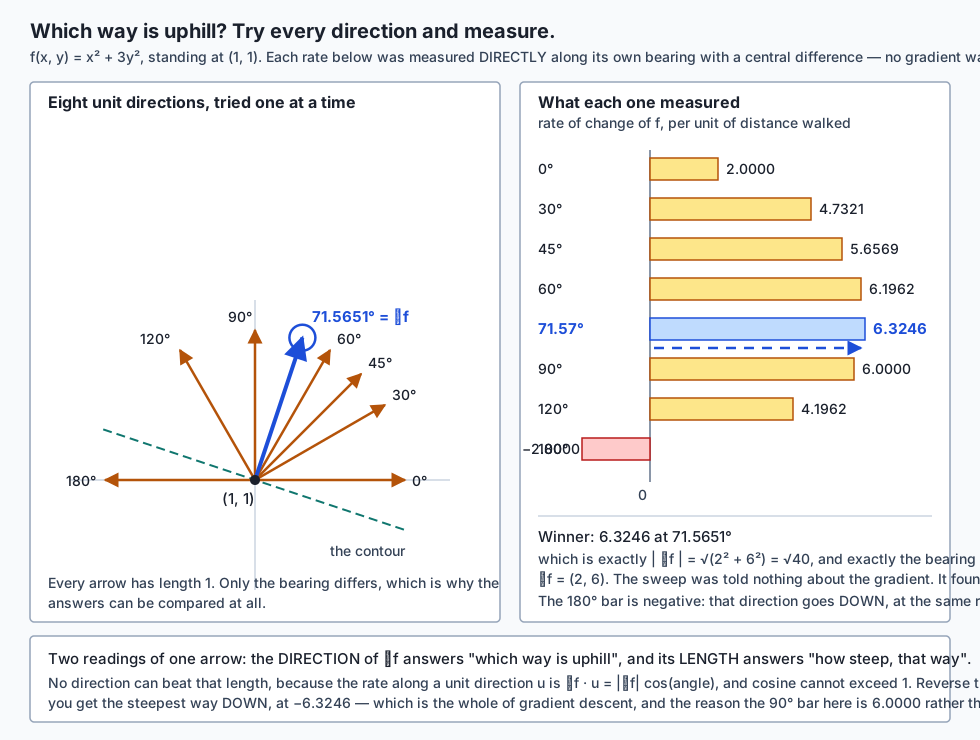
Stand at (1, 1) on the bowl, where the gradient is (2, 6) with length √40 = 6.324555 and bearing 71.5651°. Now ignore all of that and measure. Pick 360 bearings, one per degree. For each one, take a central difference along that bearing directly — step h forward, step h back, divide by 2h. The gradient plays no part in producing these numbers.
   surface          point   best bearing   gradient bearing       gap     best rate    |gradient|
      bowl     (1.0, 1.0)          72.0d           71.5651d   0.4349d     6.3243731     6.3245553
      bowl   (0.25, 0.75)          84.0d           83.6598d   0.3402d     4.5276128     4.5276926
   product    (2.0, -1.0)         117.0d          116.5651d   0.4349d     2.2360035     2.2360680
    saddle     (1.5, 0.5)         342.0d          341.5651d   0.4349d     3.1621865     3.1622777
     cubic     (1.0, 1.0)          27.0d           26.5651d   0.4349d     4.4720071     4.4721360
     plane    (-2.0, 4.0)         326.0d          326.3099d   0.3099d     3.6054985     3.6055513
The sweep finds the gradient without being told about it, on every surface tried.
The gap is not zero and cannot be, and it is worth understanding why rather than treating it as slop. With one sample per degree, the closest sampled bearing to any given angle is at most half a degree away. That is a property of the sampling grid, not of the calculus, and it is why the lab’s tolerance is one degree rather than something tighter.
The sharper check is the one in the last two columns. If D_u f = |∇f| cos θ, then the winning rate divided by |∇f| should equal the cosine of the sampling gap — not approximately, but to as many decimal places as float64 has:
   surface          point    best rate / |grad|            cos(gap)    difference
      bowl     (1.0, 1.0)        0.999971186303      0.999971186304      2.51e-13
      bowl   (0.25, 0.75)        0.999982373301      0.999982373300      1.15e-12
     plane    (-2.0, 4.0)        0.999985369501      0.999985369545      4.33e-11
That is the geometric dot product, checked as an identity rather than quoted as a slogan.
Two more things fall out of the same sweep. The direction with the most negative rate is exactly 180° round from the winner, and its rate is the exact negative — which is Day 111 in one sentence: to go down, step against the gradient. And the two bearings where the rate is nearest zero are 90° from the gradient, one on each side. Walking either of those keeps f unchanged to first order, which means they run along the contour.
Demonstrating perpendicularity — carefully
That last observation is suggestive, not conclusive, so the lab checks perpendicularity separately and independently.
The trap here is real and worth naming. The obvious demonstration is: take the gradient, rotate it ninety degrees, call that “the contour direction”, and observe that the two are perpendicular. That proves nothing whatsoever. It is perpendicular because it was constructed to be.
So every contour used is an exact algebraic curve, derived on paper from the function alone, with the gradient nowhere in its derivation. For the bowl x² + 3y² = L:
x = √L · cos t y = √(L/3) · sin tSubstitute back: L cos²t + 3(L/3) sin²t = L(cos²t + sin²t) = L, for every t. No gradient anywhere. And before the curve is used for anything, the lab evaluates f at eight points along it and checks the drift — measured at 1.332e-15, which is float64 saying “identical”.
Now take two points on that curve, at parameters t and t + δ, and dot the unit vector between them with the unit gradient at the first. The answer is not zero, and it should not be expected to be: a chord is not a tangent, and it is tilted away from the tangent by an angle of roughly δ.
So the evidence is not one small number. It is the number shrinking:
    surface      delta    unit gradient . unit chord   ratio to previous
       bowl      1e-02             -4.7195737669e-03
       bowl      1e-03             -4.7310204493e-04              9.9758
       bowl      1e-04             -4.7321678200e-05              9.9976
       bowl      1e-05             -4.7322899418e-06              9.9997
       bowl      1e-06             -4.7325147645e-07              9.9995
Divide the step by ten, divide the dot product by ten. That is what “it goes to zero” looks like when every step you can take is finite: not a small number, but a number that shrinks at exactly the rate the geometry predicts.
And if you use the exact tangent instead of a chord, the residual disappears completely. Differentiate the parametrisation to get p'(t) = (−√L sin t, √(L/3) cos t), and dot it with the exact gradient (2x, 6y) = (2√L cos t, 6√(L/3) sin t):
−2L·sin t·cos t + 6·(L/3)·sin t·cos t
  = (−2L + 2L)·sin t·cos t
  = 0
Identically zero, for every t and every level. The lab prints 0.000e+00 at six different parameter values. The small numbers above are an artefact of measuring with finite steps, not a hedge.
A zero gradient, and the three things it cannot tell you
Three surfaces, all with ∇f = [0, 0] at the origin:
| Surface | ∇f at origin | What the origin actually is |
|---|---|---|
x² + 3y² | [0, 0] | a minimum — every direction goes up |
−(x² + y²) | [0, 0] | a maximum — every direction goes down |
x² − y² | [0, 0] | a saddle — up along x, down along y |
Walk 0.1 in eight directions from each origin and record what f does:
      surface        0d       45d       90d      135d      180d      225d      270d      315d
         bowl   +0.0100   +0.0200   +0.0300   +0.0200   +0.0100   +0.0200   +0.0300   +0.0200
         dome   -0.0100   -0.0100   -0.0100   -0.0100   -0.0100   -0.0100   -0.0100   -0.0100
       saddle   +0.0100   +0.0000   -0.0100   -0.0000   +0.0100   +0.0000   -0.0100   -0.0000
Same gradient, three completely different situations. And this is not a limitation of how carefully you compute the gradient — no amount of precision would help, because the information is not in there. The gradient is built from first derivatives; which kind of stationary point this is depends on the second ones. That object is the Hessian, and this course does not develop it here.
The saddle’s four zero entries are not rounding, incidentally. On x² − y² the diagonals are exactly where x² = y², so f is unchanged along them. Those are the two contour lines that cross at the saddle, which is what makes a saddle a saddle.
Why saddles matter enormously. In two dimensions a saddle is a curiosity. In the parameter space of a model there are not two directions but millions, and being a minimum requires the surface to curve upward in every single one of them at once, while being a saddle requires only one to disagree. As the number of parameters grows, a stationary point is overwhelmingly more likely to be a saddle than a true minimum. An optimiser that stops when the gradient is zero would stop at a place it could have escaped by moving a millimetre in one direction out of a million — and the practical version is worse than the clean one, because near a saddle the gradient is small without being zero, so progress crawls rather than stopping, and from the outside a crawl looks a lot like convergence.
      distance from the saddle    |gradient|
                           1.0      2.828427
                           0.1      0.282843
                          0.01      0.028284
                         0.001      0.002828
An everyday analogy
The analogy that carries this whole day is a walking map with contour lines on it, and it is worth spending a paragraph on because it is not a decoration — it is the picture every optimisation diagram in the rest of this course is literally drawn as.
You are on a hillside in fog, holding a map. The map is flat, and on it are closed loops — contour lines, each one joining points of equal height. Where the loops are close together the ground is steep; where they are far apart it is gentle. You cannot see the hill. You can only feel the ground immediately around your boots.
The partial derivatives are what you learn by taking one careful step in each of two fixed directions. Step due east, note whether you went up or down and by how much, step back. Step due north, same. Two numbers.
The gradient is the arrow you can then draw on the map, and here the analogy earns its keep in three ways at once.
It is drawn on the map — flat, two components, a direction to walk — not sticking up out of the hillside. The height lives on the paper as contours, not as a third arrow.
It points straight uphill, which you did not measure and could not see in the fog. You measured east and north; the arrow knows about north-north-east. That is the compression, and it is genuinely surprising the first time.
And it crosses the contour lines at right angles. On a real map you can check this with a protractor: the steepest way up a slope is always square to the contour, because walking along a contour is walking on the level, and any direction with something to gain must have some component across it.
Two extensions of the analogy are worth having.
The length of the arrow is the steepness, and it changes. Far out on a wide hillside the arrow is long; near the summit it shortens; at the top it vanishes. That vanishing is why gradient descent takes smaller steps as it approaches the answer, without anyone telling it to.
And the arrow does not necessarily point at the summit. This is where most people’s intuition quietly breaks, and the bowl x² + 3y² makes it visible: it is elliptical rather than circular, so from (1, 1) the negative gradient points along a bearing of 251.565° while the minimum is at 225°. Twenty-six and a half degrees off. Steepest-downhill and straight-towards-the-bottom are different directions, and the gap between them is exactly what makes gradient descent zig-zag down a narrow valley instead of walking calmly in. Day 111 will watch it happen.
Where the analogy stops: a real hillside has two input dimensions because that is how many the ground has. A loss surface has as many as the model has parameters. There is no fog thick enough to make a million-dimensional landscape hard to picture, because you cannot picture it at all. Everything in this section survives the move except the picture itself, and that is precisely why the picture is worth learning properly first.
Examples in practice
A partial derivative that catches everybody
f(x, y) = xy, at the point (1, 0).
             point   df/dx exact          measured   df/dy exact          measured
        (1.0, 0.0)        0.0000    0.000000000000        1.0000    1.000000000000
        (1.0, 1.0)        1.0000    1.000000000001        1.0000    1.000000000001
        (1.0, 5.0)        5.0000    4.999999999988        1.0000    0.999999999962
       (3.0, -2.0)       -2.0000   -2.000000000013        3.0000    3.000000000064
Read the first row again. The slope in x is exactly zero, and the surface is anything but flat there — the slope in y is 1. Walk along the x-axis and f is identically zero the whole way, so of course the x-slope is zero; step off that line by a hair and it stops being zero. A single partial derivative is a statement about one direction, and it is not a statement about the point.
Where a numerical gradient stops working
This section was not planned. It exists because an assertion failed while the lab was being built, and it turned out to be more useful than the tidy version would have been.
A plane’s gradient is constant, so a numerical estimate ought to be equally good anywhere. It is not:
                       point            |f|    measured df/dx        error    eps|f|/2h
                  (1.0, 1.0)            6.0      3.0000000000    1.965e-11    6.661e-11
               (-40.0, 17.5)          150.0      3.0000000010    9.522e-10    1.665e-09
           (1000.0, -1000.0)         5005.0      3.0000000152    5.052e-08    5.557e-08
       (100000.0, -100000.0)       500005.0      2.9999995604    3.587e-06    5.551e-06
   (10000000.0, -10000000.0)     50000005.0      3.0003488064    3.488e-04    5.551e-04
The reason is entirely in the last column. The central difference computes (f(x+h) − f(x−h)) / 2h, and each stored value of f carries a relative error of about one machine epsilon. At (1000, −1000), f is worth about 5005, so each value’s absolute error is around 5005 × 2.2e-16. The subtraction preserves that error while the division by 2h = 2e-5 multiplies it by fifty thousand. Predicted noise: ε|f| / 2h — and the prediction tracks the measurement across seven orders of magnitude.
By ten million, an estimate of a gradient that is exactly 3 has lost its fourth decimal place. Nothing about the calculus went wrong; only the arithmetic.
The lab’s response to this is the part worth copying. It would have been easy to widen the tolerance from 1e-8 to 1e-6 and move on. Instead there is a test named test_the_numerical_gradient_stops_meeting_the_labs_tolerance_far_from_home which asserts the failure, so the boundary is documented by the suite rather than discovered later by someone else. A check that has been widened until it cannot fail is worse than no check, because other people will rely on it.
numpy.gradient, which is a different job
NumPy has a function called gradient, and reaching for it here would be a mistake — not because it is bad, but because it answers a different question. Ours takes a function and a point. NumPy’s takes an array of values already sampled on a grid.
On a 9×9 grid over [0, 4]² sampling x² + 3y², with spacing 0.5:
    interior sample at (x, y) = (1.0, 1.0): numpy [2.000000, 6.000000]  exact [2.000000, 6.000000]
    corner sample at (0.0, 0.0):  numpy [0.500000, 1.500000]   exact [0.0, 0.0]
    the same corner with edge_order=2: [0.000000, 0.000000]   exact, this time
The interior is exact, because a central difference is algebraically exact on a quadratic at any spacing. The corner is wrong — (0.5, 1.5) where (0, 0) is correct — because numpy.gradient defaults to edge_order=1, a first-order one-sided formula at the boundary. Nothing warns you. Passing edge_order=2 fixes it exactly. That default is worth knowing about before it costs you an afternoon, and the lab asserts both behaviours so that a future release changing either would fail the suite rather than let this page go quietly stale.
The deeper difference shows on a cubic:
    at (x, y) = (2.0, 2.0), exact df/dx = 16.0
      numpy.gradient on the sampled array :  16.2500000000   error 2.500e-01
      grid spacing squared                 :   0.2500000000
      our gradient, on the function itself :  16.0000000003   error 2.825e-10
Same h² law — but h is now the grid spacing, fixed by the data you were handed. You cannot shrink it without resampling, and if the samples came from a sensor you may not be able to at all. So: numpy.gradient when you have an array of values — an image, a height field, a measured series. A gradient like today’s when you have a function you can call. They are not competitors.
Implications: security, privacy, performance, scalability, and cost
Performance and cost. A numerical gradient of a function of n inputs costs exactly 2n evaluations of the whole function. That is arithmetic, and the lab counts it by wrapping the loss in a call counter. In units of complete forward passes through a model:
| Parameters | Forward passes for ONE numerical gradient |
|---|---|
| 3 | 6 |
| 1,000 | 2,000 |
| 1,000,000 | 2,000,000 |
| 1,000,000,000 | 2,000,000,000 |
A million-parameter model would need two million complete forward passes to take one training step. Training takes millions of steps. The method you build today is, at that scale, not slow — it is impossible, by a margin of many orders of magnitude. This is the single most important number in the lesson, and the alternatives section is about what replaced it.
Scalability, in a subtler sense. The failure above is about the number of inputs. There is a second scaling failure about the size of the output, shown in the examples section: roundoff error grows in proportion to |f|, so a loss of a hundred thousand gives you four good digits where a loss of ten gives you eleven. Scaling your inputs and outputs to sensible magnitudes before differentiating anything is not fussiness; it is the difference between a usable answer and a confident wrong one.
Security. A numerical gradient calls the function you hand it, 2n times. If that function does anything other than compute a number, that thing happens 2n times: 2n file writes, 2n remote requests, 2n charges to an account — and Day 111 will call gradient inside a loop. The general shape is that a function passed as a value is executed on somebody else’s schedule, not yours. Counting the calls before committing to them is a two-line habit worth having.
The second security-shaped concern is the tolerance one from the examples section, and it generalises well beyond calculus. When a check starts failing, the tempting fix is to loosen it until it passes. A check that cannot fail still reports a green tick, and people build on that tick. Widening a tolerance to hide a real limit converts a test into decoration, and it is the same reasoning that lets a misconfigured security control pass review.
Privacy. Nothing today touches personal data, but one implication is worth flagging early because it becomes a serious topic later in this course: gradients carry information about the data that produced them. A gradient of a loss with respect to parameters is computed from training examples, and it is not a one-way summary — in some settings the inputs can be partially reconstructed from it. Anywhere gradients cross a trust boundary, which is exactly what happens in federated learning, that is a disclosure channel and not merely a number.
Cost, in the ordinary sense. Nothing in today’s lab costs money. Two free, open-source packages, no account, no key, no service. The compute is negligible: the largest object anywhere in the lab is a 9×9 grid.
Alternatives: free, open source, and commercial
Four routes to a gradient. Only the first two were run here, and the lesson says which is which rather than implying a test that did not happen.
1. Your own numerical gradient — what today builds. Run here. Free, no dependency beyond arithmetic. Choose it when you have a function you can call and no way to see inside it — a black box, a simulator, a legacy binary — or when you need to check a gradient someone else computed. It works on anything callable, needs no cooperation from the function, and takes about ten lines. It costs 2n evaluations, is accurate to roughly h² rather than exactly, and degrades as |f| grows. Concretely: gradient(model_loss, (1.0, 1.0, 1.0)) returned [-17.0, -18.0, -8.0] against a hand-derived exact [-17, -18, -8], in six evaluations of the loss.
2. numpy.gradient — a different job. Run here. Free, BSD 3-Clause, part of NumPy. Choose it when you have an array of already-sampled values rather than a function: an image, a heightmap, a time series, the output of a simulation you cannot re-run. It gives you the gradient at every grid point at once, which is exactly what you want for edge detection or a flow field, and it cannot be asked for a value between grid points. Its accuracy is fixed by the sampling you already have — the lab measured its error on a sampled cubic at 0.25, which is the grid spacing squared — and its edge_order defaults to 1, so boundary values are first-order. Concretely: np.gradient(Z, xs, ys) on a sampled x² + 3y² returned [2.0, 6.0] in the interior, exactly right, and [0.5, 1.5] at a corner where [0, 0] is correct.
3. Symbolic differentiation, such as SymPy. Not installed here; described from its documentation, and no output is reproduced. Free and open source. You hand it an expression and it hands you back another expression — the exact derivative, as algebra, which you can read, simplify and evaluate anywhere at full precision. Choose it when the function is small enough to write down and you want the formula rather than a number, which is exactly the situation when you are deriving something for a paper or checking your own algebra. It does not scale to a model: symbolic derivatives of deeply composed functions suffer expression swell, where the formula grows explosively even though the value is cheap to compute.
4. Automatic differentiation — PyTorch’s autograd, JAX’s grad. Not installed here; described from their documentation, and no output is reproduced. Both free and open source; the commercial dimension is the hardware and the managed platforms they run on rather than the libraries themselves. This is what every training loop in the world actually uses, and it is neither of the two things above. It is not symbolic — no formula is ever built. It is not numerical in today’s sense — no h, no subtraction of nearby values. It records the operations your function performed and applies the chain rule (Day 110) to that record.
Two properties follow, and they are precisely the two failures of the method you build today.
It is exact. Not accurate to h² — exact, up to floating-point rounding of the operations themselves. There is no step size to choose, no U-curve, and no degradation as |f| grows.
Its cost does not scale with the number of parameters. Reverse-mode autodiff gets the entire gradient for a cost of roughly one forward pass plus one backward pass, regardless of whether there are three parameters or a billion. Compare that with the 2n in the table above. This is not an optimisation of numerical differentiation; it is a different algorithm with different asymptotics, and it is the reason training a large model is possible at all.
So why build the slow one? Because numerical differentiation has one job left that autodiff cannot do for itself: checking it. If your hand-written backward pass disagrees with a numerical gradient on a small example, the hand-written one is wrong. That check has a name — gradient checking — and today’s lab is a working implementation of it. It is the standard first move when a custom layer trains badly, and it is why this method is in every serious deep-learning toolkit even though nothing trains with it.
Comparison with related concepts
| Concept | Input | Output | What it tells you | Where you met it |
|---|---|---|---|---|
Derivative df/dx | one number | one number | the slope of a curve | Day 108 |
Partial derivative ∂f/∂xᵢ | several numbers | one number | the slope along one axis, others frozen | today |
Directional derivative ∇f · u | several numbers + a unit direction | one number | the slope along any chosen bearing | today |
Gradient ∇f | several numbers | a vector | steepest ascent, and how steep | today |
| Jacobian | several numbers | a matrix | how each of several outputs responds to each input | Day 110 names it |
| Hessian | several numbers | a matrix | curvature — whether a stationary point is a min, max or saddle | named, not developed |
Four distinctions are worth stating explicitly, because each one is a place people get stuck.
Derivative versus partial derivative. These differ in bookkeeping, not in mathematics. If f has one input, df/dx and ∂f/∂x are the same number and the second notation is just noise. The ∂ only starts meaning something when there is a second variable to hold still.
Partial derivative versus directional derivative. A partial derivative is a directional derivative, taken along an axis. ∂f/∂x is the rate along (1, 0); ∂f/∂y is the rate along (0, 1). The lab measures this directly: at (1, 1) on the bowl, ∇f · (1,0) = 2.0 and ∇f · (0,1) = 6.0, which are the two partials.
Gradient versus a list of partial derivatives. Numerically these are the same numbers. Conceptually the gradient is the claim that those numbers form a vector — that they transform correctly, have a meaningful length and direction, and can be dotted with things. That claim is what the whole day’s demonstrations are about, and it is not free: the counterexample in the “what it is not” section is a function whose partials all exist and which nonetheless has no vector worth calling a gradient at one point.
Gradient versus Jacobian. A gradient is what you get when the function returns one number. When it returns several, each output gets its own gradient, and stacking them as rows gives the Jacobian. So the gradient is the one-row case. This matters for Day 110, because the chain rule for composed multi-output functions is a chain of matrix products.
When to use it — and when not to
Use a numerical gradient when:
- the function is a black box you can call but not read — a compiled binary, a simulator, a service;
- you need to check an analytic or hand-written gradient, which is the job it is genuinely best at;
- the number of inputs is small — a dozen, not a million — so
2nevaluations is affordable; - you are learning, and want to see the definition working rather than trust a library.
Do not use one when:
- you are training a model.
2nforward passes per step makes this impossible past a few hundred parameters, and reverse-mode autodiff exists. - the function’s values are large. Roundoff error scales with
|f|, and past about1e5you are losing digits you probably need. Scale first. - the function is noisy, stochastic, or not smooth. Differencing a noisy function amplifies the noise by
1/2h, which is fifty thousand at the default step. A minibatch loss is noisy in exactly this way. - the function has a kink at the point of interest.
|x|at zero has no derivative and a central difference will hand you0without comment, which is a plausible-looking answer to a question with no answer. - you can write the derivative down. A symbolic derivative is exact, free at run time, and re-derivable by anyone reading your code.
Use the gradient — the concept — essentially always. Every optimiser you will meet is built on it, every loss curve you look at is a projection of a gradient’s behaviour, and the language of the whole field assumes it.
Where this goes next in AI work
Here is the AI thread, and it is a single sentence with a large consequence: every parameter of a model gets a partial derivative, and the gradient is that entire collection — one number per weight, millions of them.
Nothing about that is a metaphor. Take the smallest thing that is honestly a model — a prediction w₁a + w₂b + c and a mean-squared-error loss over four samples. That loss is a function of three inputs, and they are not the data. The data is fixed. What varies, and what the derivative is taken with respect to, is the parameters. This swap is the thing to hold on to: in ∂L/∂w₁, the features a and b are constants and w₁ is the variable.
At w₁ = w₂ = c = 1 the loss is 22.5 and the gradient is:
     parameter           numerical   exact, by hand        error
            w1    -16.999999999889         -17.0000    1.107e-10
            w2    -17.999999999851         -18.0000    1.485e-10
             c     -7.999999999697          -8.0000    3.029e-10
Three parameters, three partial derivatives. A network with a hundred million parameters differs from this in exactly one respect: the number of parameters. Same definition, same meaning, same vector — one hundred million entries long.
And the gradient is still a vector, so everything from Day 99 still applies. It has a length (26.019224 here). It has a unit version. There is no picture — the input space has three dimensions and the graph would need four — but every statement from the two-dimensional case survives the move: it points the steepest way up, its length says how steep, and it is perpendicular to the level set, which is now a surface rather than a curve. That transfer is the whole reason today was spent on pictures of hills.
Step against it and the loss falls. Not as a claim — as a measurement:
   step size                      new parameters            loss        change
   0 (start)   [  1.00000,   1.00000,   1.00000]     22.50000000
       0.001   [  1.01700,   1.01800,   1.00800]     21.82819150     -0.671808
       0.010   [  1.17000,   1.18000,   1.08000]     16.24915000     -6.250850
       0.050   [  1.85000,   1.90000,   1.40000]      1.62875000    -20.871250
       0.100   [  2.70000,   2.80000,   1.80000]      6.71500000    -15.785000
       0.200   [  4.40000,   4.60000,   2.60000]     94.76000000    +72.260000
The direction is right at every step size. How far to go along it is a separate question with its own name — the learning rate — and its own way of going badly wrong: at 0.2 the loss ends up four times worse than where it started. Day 111 is about both, and it is now three lines away from what you already have.
Knowledge check
Eight questions on the day’s material — the definition of a partial derivative, what the gradient’s length and direction each mean, why the gradient is perpendicular to the contour, and what a zero gradient does and does not tell you. Two of them are the ones this lesson would most like you to get right, and neither is about computing anything.
Hands-on exercise
The lab is “Which Way Is Uphill?”. Start from its README.md, then starter/00_brief.md.
You write eight functions in starter/gradients.py and fifty-one predictions in starter/answers.py. The first two functions are the day:
def partial(f, point, index, h=1e-5):
    """Nudge ONE coordinate each way, hold the rest still, divide by 2h."""

def gradient(f, point, h=1e-5):
    """One partial per input, collected into a vector."""
Everything else — magnitude, unit, both directional derivatives, the 360-direction sweep, the forward difference — is built out of those two. Write partial first and get its tests green before anything else; three of them exist specifically to catch the three ways it goes wrong.
Then thirty-two further tests run automatically against the functions you already wrote, and they are the two facts the day exists for: that the gradient wins a sweep of 360 directions, and that it is perpendicular to an exactly parametrised contour.
Expected output
An untouched checkout:
1 passed, 205 skippedA finished one:
206 passedAnd the full harness:
98 checks, 0 failure(s).with exit status 0. The reference suite in examples/ runs 271 tests.
Validate your work
bash tests/run_tests.sh; echo "exit=$?"prints98 checks, 0 failure(s).andexit=0..venv/bin/pytest examples -q -p no:cacheproviderprints271 passed..venv/bin/pytest starter -q -p no:cacheproviderprints206 passedwhen you are done.- Each of the seven reference scripts ends with
every assertion held. find . -path ./.venv -prune -o -type d -name '__pycache__' -printprints nothing.
The harness also proves it can fail: section 6 re-runs the whole script with one expectation swapped for the belief that a bowl’s gradient at (1, 1) points at 45° — straight away from the minimum — rather than at its true 71.5651°, and asserts that the re-run exits non-zero and reports exactly one failure.
Troubleshooting
ModuleNotFoundError: No module named 'gradients' — run the reference scripts from inside examples/; they import from beside themselves.
Every partial exactly twice too big — you divided by h instead of 2h.
Partials right in x and nonsense in y — you modified the point in place instead of copying it, so the first nudge is still there when the second runs.
ValueError: the zero vector has no direction — you asked for the unit vector of a zero gradient, which happens at exactly the interesting points. That is the function working.
A gradient assertion fails, but only far from the origin — expected. See the examples section above; do not widen the tolerance.
The sweep misses the gradient bearing by 0.4349° — expected, and it is half the sampling step plus a little. Sample 3600 directions and it drops below 0.05°.
The contour dot product is not zero — expected. A chord is not a tangent. The evidence is that it shrinks tenfold when the step shrinks tenfold.
troubleshooting.md in the lab covers all of these plus five more, every one hit while building it.
Common mistakes
Giving a two-input function a three-component gradient. The gradient lives in the input space. Two inputs, two components, however many dimensions the graph occupies.
Forgetting to normalise the direction in a directional derivative. Then a longer arrow gives a bigger answer and the quantity means nothing.
Reading a zero partial derivative as a flat point. ∂f/∂x = 0 at (1, 0) on f = xy, where ∂f/∂y = 1.
Reading a zero gradient as a minimum. It is a stationary point, and it might be any of three things.
Tuning a tolerance until the test passes. Every tolerance in the lab is derived in surfaces.py from what the arithmetic can achieve, and one test asserts a failure rather than papering over it.
Demonstrating perpendicularity by rotating the gradient. True by construction, and therefore no evidence at all.
Practice assignment
Work these in the lab directory, using the functions you wrote.
-
A new surface, start to finish. Add
f(x, y) = x² + xy + 2y²to a copy ofsurfaces.py. Derive∇fby hand — remember that thexyterm contributes to both partials. Check your numerical gradient against it at five points. Then find the point where the gradient is zero by reasoning rather than searching, and confirm it. -
The steepest-ascent property, on your surface. Run the 360-direction sweep at three points on it. For each, report the winning bearing, the gradient’s bearing, and the gap, and confirm the gap never exceeds half a degree. Then sweep 36 directions instead and predict the new bound before you measure it.
-
A contour you derive yourself. The contours of
x² + xy + 2y²are ellipses, but tilted. Rather than deriving the tilt, find points on one contour numerically: fix a level, pick an angle, and solve along a ray from the origin for the radius that lands on that level. Then check perpendicularity with chords, and confirm the dot product falls tenfold per tenfold smaller step. -
Your own U-curve. Sweep
hfrom1e-1to1e-14on your surface at a point where|f|is around 10, then again where|f|is around 10,000. Report both troughs. Predict, before measuring, whether the second trough moves left or right, and explain why in one sentence aboutε|f|/2h. -
A four-parameter model. Extend
model_losstow₁a + w₂b + w₃ab + c. Derive all four partials by hand, check them numerically, and count the evaluations. Then take one step against the gradient at five step sizes and report the loss at each. -
Write the honest paragraph. In no more than 200 words, explain to someone who has done Day 108 but not today why the gradient’s length is a rate rather than a distance, and why a zero gradient does not mean you have finished. Use no equation.
Extension challenge
Build a gradient checker, and then make it catch something.
Write check_gradient(loss, point, analytic_gradient) that computes the numerical gradient, compares it component by component against the analytic one supplied, and returns a per-component relative error rather than an absolute one — because the whole point of today’s ε|f|/2h finding is that an absolute tolerance does not travel.
Then earn it. Take model_loss_gradient from the lab, introduce a single sign error into one component, and confirm that your checker finds it, names which parameter is wrong, and reports an error large enough that nobody could mistake it for roundoff. Then introduce a subtler bug — a factor of 2 missing from one term — and check that it is still caught.
Finally, the part that makes this a real tool: decide what threshold separates “this gradient is wrong” from “this is floating-point noise”, and justify the number. You have everything you need from today. The relative error of a correct numerical gradient at a well-scaled point is around 1e-10; the smallest interesting bug — a missing factor of 2 — produces a relative error of about 0.5. There are nine orders of magnitude of daylight between them, which means your threshold does not have to be clever, and being able to say why it does not have to be clever is the whole skill.
If you want to push further: make the checker report which single component has the worst relative error and print the numerical and analytic values side by side, then run it on a function whose analytic gradient is correct but whose loss is badly scaled — say, multiplied by 1e6 — and watch a correct gradient get flagged. Working out what to do about that is the same problem as the one in the examples section, and there is no answer that does not involve scaling something.
Quiz
Q1. On `f(x, y) = xy` at the point `(1, 0)`, the partial derivative `∂f/∂x` is exactly 0. What does that tell you about the surface at that point?
- Very little on its own — it says the slope is zero along the x direction, and `∂f/∂y` there is 1, so the surface is not flat at all
- The surface is flat at that point, since a zero derivative means no change
- The point is a minimum of the function
- The function is not differentiable there, which is why the partial is zero
Show answer
Answer: A. Very little on its own — it says the slope is zero along the x direction, and `∂f/∂y` there is 1, so the surface is not flat at all
A partial derivative is a statement about ONE direction, not about the point. Walk along the x-axis, where y is 0, and `f = x × 0 = 0` the whole way — the function is identically zero along that line, so of course its slope along it is zero. Step off the line by a hair and it stops being zero: `∂f/∂x = y`. Meanwhile `∂f/∂y = x = 1` at that point, so the ground is climbing at unit rate in the perpendicular direction. Option 1 is the intuition carried over from one-variable calculus, where a zero derivative really does mean the curve is level; with several variables you need EVERY partial to vanish before the ground is level, and even then see question 5. Option 2 is wrong for the same reason and also because `f = xy` takes negative values arbitrarily close to `(1, 0)`. Option 3 is wrong: `xy` is a polynomial and is differentiable everywhere.
Q2. For `f(x, y) = x² + 3y²`, the gradient at `(1, 1)` is `[2, 6]`. How many components does the gradient have, and why?
- Three, matching the three dimensions the graph of the function occupies
- One, because f returns a single number
- Two, matching the two INPUTS — a gradient is an arrow on the flat map you are standing on, not one pointing out of the hillside
- It depends on the step size h used to compute it
Show answer
Answer: C. Two, matching the two INPUTS — a gradient is an arrow on the flat map you are standing on, not one pointing out of the hillside
This is the most common way to misread the object, and it is worth being emphatic. The function takes a point with two coordinates and returns one number, so its graph is naturally drawn as a surface in three dimensions — and the gradient still has two components. It lives in the INPUT space. It is a direction to walk, drawn on the flat contour map, not a vector pointing up out of the terrain. The general rule: a scalar function of n inputs has an n-component gradient, whatever its graph looks like. Option 0 is the mistake this question exists to catch. Option 1 confuses the gradient with the function value. Option 3 confuses accuracy with shape — h changes how good the numbers are, never how many of them there are.
Q3. You are at a point where `|∇f| = 6.3246`. You walk along a unit direction that makes a 60° angle with the gradient. What rate of change do you experience?
- 6.3246, because the gradient's magnitude is the rate of change in every direction
- About 3.1623, which is 6.3246 × cos(60°)
- About 5.4772, which is 6.3246 × sin(60°)
- 0, because any direction other than the gradient gives no change
Show answer
Answer: B. About 3.1623, which is 6.3246 × cos(60°)
The directional derivative is `∇f · u`, and Day 103's geometric reading of the dot product gives `|∇f| |u| cos θ`. Since u is a unit vector, `|u| = 1`, so the answer is `|∇f| cos θ` — here `6.3246 × 0.5 = 3.1623`. Wikipedia's article on the gradient offers the same arithmetic as a road on a hill: if the steepest slope is 40%%, a road at 60° from the uphill direction has a slope of "40%% times the cosine of 60°, or 20%%". Option 0 forgets that the rate depends on which way you walk, which is the entire subject of the day. Option 2 uses sine, which would give zero along the gradient itself and the maximum perpendicular to it — exactly backwards. Option 3 is the over-correction: only directions at exactly 90° give zero, and cos(60°) is 0.5, not 0.
Q4. Why is the gradient perpendicular to the contour line through a point?
- It is a convention of how contour maps are drawn rather than a mathematical fact
- Because contour lines are always straight, and gradients are always at right angles to straight lines
- It is true only for circular contours; on an elliptical bowl the angle is slightly less than 90°
- Because a contour is where f does not change, the rate along it is zero, and `∇f · u = 0` means the two vectors are perpendicular
Show answer
Answer: D. Because a contour is where f does not change, the rate along it is zero, and `∇f · u = 0` means the two vectors are perpendicular
The argument is three steps and needs no new machinery. A contour — or level set — is by definition the set of points where f takes one fixed value, so walking along it changes f by nothing. The rate of change along a unit direction u is `∇f · u`. Setting that to zero for a direction along the contour gives a dot product of zero, and a dot product of zero between two non-zero vectors is precisely what perpendicular means. Wikipedia puts it the same way: "the dot product `(∇f)ₓ · v` ... gives the directional derivative ... It follows that in this case the gradient of f is orthogonal to the level sets of f." Option 0 has it backwards — the drawing convention follows the fact. Option 1 is false; contours are only straight for a linear function. Option 2 is a tempting hedge and is wrong: the lab checks an ELLIPTICAL contour, `x² + 3y² = 4`, and the exact tangent dotted with the exact gradient is `−2L sin t cos t + 2L sin t cos t = 0` identically, for every point on it. What IS true on an ellipse is that the gradient does not point at the centre — which is question 7.
Q5. Three surfaces all have `∇f = [0, 0]` at the origin: `x² + 3y²`, `−(x² + y²)`, and `x² − y²`. What can the gradient tell you about which is which?
- Nothing — all three are stationary points and the gradient is identical; distinguishing them needs the second derivatives
- The sign of the gradient distinguishes them, but you have to look at the components separately
- Computing the gradient with a smaller h would separate them
- The magnitude of the gradient is slightly different in each case if you measure precisely enough
Show answer
Answer: A. Nothing — all three are stationary points and the gradient is identical; distinguishing them needs the second derivatives
They are a minimum, a maximum and a saddle, and the gradient is `[0, 0]` for all three. This is not a limitation of precision — it is a limitation of what a gradient IS. The gradient is built from FIRST derivatives, which describe the tangent plane; at a stationary point the tangent plane is level in all three cases and there is nothing left to distinguish. Which kind of point it is depends on the SECOND derivatives, and the matrix of those is the Hessian. Options 2 and 3 are the same mistake in two costumes: they imagine the information is present but faint. It is absent. Wikipedia names the general case: "a point where the gradient is the zero vector is known as a stationary point". The practical consequence is large — an optimiser that stops when the gradient is zero would stop dead at a saddle, and in a parameter space with millions of directions a stationary point is far more likely to be a saddle than a minimum, because being a minimum requires every one of those directions to curve upward at once.
Q6. You compute a partial derivative with a central difference and want the most accurate answer float64 can give. Which step size h is best, and what happens if you go smaller?
- The smallest representable h, since the definition involves a limit
- Around 1e-08, and going smaller improves it further
- Around 1e-05, and going much smaller makes the answer dramatically WORSE — at 1e-14 it is out by more than at h = 0.1
- It does not matter; the central difference is exact at any h
Show answer
Answer: C. Around 1e-05, and going much smaller makes the answer dramatically WORSE — at 1e-14 it is out by more than at h = 0.1
Two errors pull in opposite directions. The truncation error of a central difference shrinks like h², and the roundoff error from subtracting two nearly equal floats GROWS like 1/h — so the total is U-shaped and there is a trough. Balancing an h² term against an ε/h term puts it near the cube root of machine epsilon, which is 6.06e-06 for float64; the lab measures the best of fifteen decades at 1e-05, the nearest power of ten. Option 0 is the intuition from the definition and is exactly the trap Day 108 set up: at h = 1e-14 the measured error is 1.450e-01, fourteen times WORSE than at h = 0.1, a step a trillion times bigger, and nothing warns you. Option 1 is the answer for a FORWARD difference, whose error shrinks like h rather than h², putting its trough near the square root of epsilon at 1.49e-08 — the lab measures 1e-08 there, three decades away from the central one. Option 3 is true for a quadratic and only a quadratic: `((x+h)² − (x−h)²)/2h = 2x` exactly. On a genuine cubic the error is exactly h².
Q7. On the elliptical bowl `x² + 3y²`, the minimum is at the origin. From the point `(1, 1)`, does the negative gradient point straight at the minimum?
- Yes — the negative gradient always points at the nearest minimum, which is what makes gradient descent work
- No, and it is off by 26.565° — steepest downhill and straight-towards-the-bottom are different directions, which is what makes gradient descent zig-zag
- No, because the negative gradient points AWAY from the minimum on any bowl
- Yes for the x component but no for the y component
Show answer
Answer: B. No, and it is off by 26.565° — steepest downhill and straight-towards-the-bottom are different directions, which is what makes gradient descent zig-zag
At `(1, 1)` the gradient is `(2, 6)`, so the negative gradient has a bearing of 251.565°, while the bearing straight back to the origin is 225°. The gap is 26.565°, and it exists because the bowl is elliptical: the 3 in front of y² makes it three times steeper in y, so the steepest way down leans harder in y than a straight line to the bottom would. On a CIRCULAR bowl the two would agree exactly, which is why circular examples give a misleading intuition. Option 0 is that misleading intuition, and the gap is precisely what makes gradient descent bounce from side to side down a narrow valley rather than walking calmly in — Day 111 will watch it happen, and the fixes for it (momentum, adaptive step sizes, preconditioning) are a large part of why optimisers have names. Option 2 has the sign backwards: the gradient points away from the minimum on a bowl, so the NEGATIVE gradient points broadly back towards it. Option 3 is not a coherent statement about a direction.
Q8. A numerical gradient using a central difference costs how many evaluations of the function, and what does that mean for training a model with a million parameters?
- Two evaluations in total, so a million-parameter model costs two forward passes per step
- Two evaluations per parameter — two million forward passes for ONE step, which is why reverse-mode autodiff exists
- One evaluation per parameter, which is affordable at any scale
- It depends on the step size h; a smaller h needs more evaluations
Show answer
Answer: B. Two evaluations per parameter — two million forward passes for ONE step, which is why reverse-mode autodiff exists
`gradient` calls `partial` once per input, and `partial` evaluates f twice — once nudged up, once nudged down. So the cost is exactly 2n evaluations of the WHOLE function, and the lab counts it by wrapping the loss in a call counter: three parameters, six evaluations. One evaluation of a model's loss is one complete forward pass over the batch, so a million parameters means two million forward passes to take a single training step, and training takes millions of steps. That is not slow; it is impossible by many orders of magnitude. Reverse-mode automatic differentiation — PyTorch's autograd, JAX's grad — gets the entire gradient for roughly one forward pass plus one backward pass regardless of the parameter count, and gets it exactly rather than to within h². Neither library is installed in this lab and no output from them is reproduced. Option 0 forgets the per-parameter loop, which is the only part that matters. Option 2 describes a forward difference, which is still linear in n and still hopeless. Option 3 confuses accuracy with cost: h changes how good each answer is, never how many evaluations there are. What numerical differentiation is still genuinely for is CHECKING an analytic gradient — gradient checking — and today's lab is a working implementation of it.
Glossary
- Partial derivative
- The derivative of a function of several variables with respect to one of them, with all the others held constant — Wikipedia's definition is exactly that. Written with a rounded d, as ∂f/∂x. It is not a different kind of derivative with different rules: freezing the other inputs turns a function of several variables into a function of one, and every rule from Day 108 then applies unchanged. The rounded symbol is a note to the reader that other inputs exist and are being held still, nothing more. For f = x² + 3y², freezing y leaves x² plus a constant, so ∂f/∂x = 2x.
- Gradient
- The vector whose components are all the partial derivatives of a scalar function, one per input, written ∇f. Its direction is the direction of steepest increase and its magnitude is the rate of increase in that direction — Wikipedia states both, and calls the magnitude "the greatest absolute directional derivative". Its formal defining property is sharper and worth knowing: it is "the unique vector field whose dot product with any unit vector v at each point x is the directional derivative of f along v". A function of n inputs has an n-component gradient regardless of how many dimensions its graph occupies: it is an arrow drawn on the flat map you are standing on, not one pointing out of the hillside.
- Nabla
- The symbol ∇, "written as an upside-down triangle and pronounced del", which denotes the vector differential operator. It is an operator rather than a number or a vector: ∇ on its own means "take the partial derivative with respect to each coordinate and stack the results", and ∇f is what you get when it is applied to a particular function. The gradient is also commonly written grad f.
- Contour line
- A curve joining points at which a function of two variables takes one fixed value — the line on a walking map that joins points of equal height. Where contours are close together the function is changing fast; where they are far apart it is nearly level. The gradient is perpendicular to the contour through every point, which is why an optimiser's path is drawn crossing the contours at right angles. Every optimisation picture in the rest of this course is a contour map.
- Level set
- The general name for the set of points where a function takes one fixed value, of which a contour line is the two-input case. For a function of three inputs it is a surface rather than a curve — Wikipedia notes that "a level surface in three-dimensional space is defined by an equation of the form F(x, y, z) = c" and that "the gradient of F is then normal to the surface". The perpendicularity result survives every increase in dimension; only the picture stops being drawable.
- Directional derivative
- The rate at which a function changes as you move from a point along a chosen direction, computed as the dot product of the gradient with the UNIT vector in that direction: D_u f = ∇f · u. Normalising first is not tidiness — without it, handing in a longer arrow would give a bigger answer and the quantity would depend on how the direction was written rather than on which way it points. A partial derivative is the special case where the direction is an axis. Since ∇f · u = |∇f| cos θ, the answer for every direction is recoverable from one gradient.
- Steepest ascent
- The direction in which a function increases fastest from a point, which is the direction of its gradient. It follows from the geometric dot product: D_u f = |∇f| cos θ, cosine cannot exceed 1, and it reaches 1 exactly when the direction is the gradient's. The largest available rate is therefore |∇f| and the most negative is −|∇f|, attained by walking exactly the opposite way — which is gradient descent. The property requires the function to be DIFFERENTIABLE, not merely to have partial derivatives; Wikipedia gives a function whose partials all exist at the origin and whose gradient formula nonetheless "fails to point towards the steepest ascent in some orientations" there.
- Stationary point
- A point where the gradient is the zero vector — Wikipedia names it as such. The ground is level in every direction to first order. The gradient carries no information at all about what KIND of point it is: a minimum, a maximum and a saddle all produce the identical zero vector, and no amount of extra precision would separate them, because the distinguishing information lives in the second derivatives rather than the first.
- Saddle point
- A stationary point that goes up in some directions and down in others — the middle of a mountain pass, or the origin of x² − y², which rises along x and falls along y. In two dimensions this is a curiosity. In a model's parameter space it is the dominant case, because being a minimum requires the surface to curve upward in every one of millions of directions simultaneously while being a saddle requires only one of them to disagree. The practical hazard is not that an optimiser stops there but that near one the gradient is small without being zero, so progress crawls, and from outside a crawl is hard to tell from convergence.
- Jacobian
- The matrix of first partial derivatives of a function that returns a VECTOR rather than a single number, with one row per output and one column per input. A gradient is the one-row case. It is named here and not developed; it becomes necessary on Day 110, because the chain rule for composed multi-output functions is a chain of matrix products.
- Hessian
- The square matrix of SECOND partial derivatives of a scalar function, with one row and one column per input. It describes curvature, and it is the object that answers the question the gradient cannot: whether a stationary point is a minimum, a maximum or a saddle. Named here and not developed. Its cost is the reason it is rarely used at scale — it has one entry per pair of parameters, so a million-parameter model would have a Hessian with a trillion entries.
- Surface
- The graph of a function of two variables, drawn as a landscape in three dimensions with the function's value as height. Wikipedia's article on partial derivatives describes the geometry precisely: at every point on such a surface there are infinitely many tangent lines, and "partial differentiation is the act of choosing one of these lines and finding its slope" — usually the ones parallel to the xz-plane and the yz-plane, which is what freezing y or x respectively produces. Beyond two inputs the surface stops being drawable, which is why the two-input picture is worth learning properly.
- Unit direction
- A vector of length exactly 1, used to specify a direction without also specifying a distance. Obtained by dividing a vector by its magnitude, which is undefined for the zero vector — a zero vector has no direction to preserve, and today's lab raises ValueError rather than returning NaNs that would surface somewhere harder to diagnose. Every directional derivative is taken along a unit direction so that the answer depends on the bearing alone.
- Central difference
- The estimate ( f(x+h) − f(x−h) ) / 2h, carried over from Day 108 and adapted here by moving only one coordinate. Its truncation error shrinks like h squared, against h for a one-sided forward difference, at a cost of one extra evaluation of f. On a quadratic it is algebraically EXACT at any h, since ((x+h)² − (x−h)²)/2h = 4xh/2h = 2x; on a cubic the error is exactly h squared with no other terms. Divide by 2h and not h: the point moved a total distance of 2h.
- Gradient checking
- Comparing a hand-written or analytic gradient against a numerical one on a small example, to find out whether the analytic one is correct. It is the job numerical differentiation is still genuinely best at, and the reason the method survives in serious toolkits long after nothing trains with it. The comparison should be relative rather than absolute, because a numerical gradient's roundoff error grows in proportion to the size of the function's values.
Sources and further reading
- NumPy documentation — NumPy Developers (accessed 2026-08-17)
- Partial derivative — Wikipedia (accessed 2026-08-17)
- Gradient — Wikipedia (accessed 2026-08-17)
- Derivative — Wikipedia (accessed 2026-08-17)
- Essence of calculus — 3Blue1Brown (accessed 2026-08-17)
- Multivariable Calculus, Fall 2007 (18.02) — MIT OpenCourseWare (accessed 2026-08-17)
Kept in this browser, no account needed. Your progress page turns the whole record into one link you can bookmark or open on another device.