Math, Statistics, and Data › Linear Algebra II and Calculus › Day 110
Day 110: The Chain Rule
After this lesson you will know why backpropagation works, and you will know it because you will have written it. The chain rule is the hinge of the whole calculus arc: Day 108 gave you a rate of change, Day 109 gave you a gradient, and today those rates get connected end to end so that Day 111 can walk downhill. The idea needs no calculus to feel. If gear A turns twice for every turn of gear B, and B turns three times for every turn of C, then A turns six times per turn of C — the rates multiplied, and that is the whole rule. You will meet composition with numbers before any derivative appears, then the chain rule stated and immediately verified against Day 108's central difference on six functions, then the dy/du times du/dx notation with an honest account of why the cancelling reading is a useful mnemonic and not a proof. You will work chains of two, three and five functions and watch the product grow without the shape changing, which is why depth is cheap. Then the part to slow down for: when a variable reaches the output by more than one route, the contributions ADD. You will see four candidate answers put to a measurement and only the sum survive, and you will learn that this single fact is what a += in an autodiff engine implements. You will meet the computation graph as the picture that makes all of this obvious, and forward versus reverse mode explained by cost rather than mechanics — reverse mode gets every input derivative from one backward pass, which is why training a model with a hundred million parameters and one loss is affordable at all. You will backpropagate a two-layer network entirely by hand, with numbers chosen so every value is exact in float64 and you can check the lot with a pen. And in the lab you will build a working reverse-mode autodiff engine in about seventy lines — the core of PyTorch's autograd, with the engineering removed — and check every gradient it produces against a numerical derivative that knows nothing about your graph. You will also measure two things that contradict the obvious answer: 0.5 to the fiftieth power does not vanish when added to 1, and a stack of forty tanh layers decays ten orders of magnitude more slowly than the standard vanishing-gradient argument predicts.
Hands-on lab for this lesson
Lab files on GitHub: https://github.com/ai-roadmap-365/ai-roadmap-365.github.io/tree/main/labs/sections/math-statistics-and-data/day-110-the-chain-rule
- Get the hands-on files. Clone the labs repository once (you can reuse this clone for every lesson). This works on macOS, Linux, and Windows (PowerShell or WSL):
git clone https://github.com/ai-roadmap-365/ai-roadmap-365.github.io.git cd ai-roadmap-365.github.io - Open this lesson's lab. Move into the directory for this specific day. Every lab lives at the same predictable path — section / subsection / week / day:
cd labs/sections/math-statistics-and-data/day-110-the-chain-rule - Read the lab guide. Open `README.md` in that directory. It lists the exact commands, what each does, the expected output, and how to check your work — read it before running anything.
- Run it and check your work. Follow the README's "How to run" section: run the example first to see the finished result, then complete the numbered exercises in `starter/`, then run the tests. The tests pass (exit 0) only when your work is correct.
bash tests/run_tests.sh # or the test command named in the lab README
You can also open the lab as a local page (works offline, shows the file tree and expected output).
Learning objectives
By the end of this lesson you will be able to:
- State the chain rule as a sentence about rates rather than as a formula, and explain the gear train that makes it obvious before any notation arrives
- Compose two functions, evaluate the composition by hand, and say which of the two runs first and why the order matters
- Apply the one-variable chain rule correctly, and explain why the outer derivative must be evaluated at the inner value rather than at x
- Verify a chain-rule result against a central difference, and say why that check is genuinely independent rather than circular
- Read the notation dy/dx = dy/du times du/dx, use the cancelling reading as a mnemonic, and state precisely why it is not a proof and where it stops working
- Differentiate a chain of any depth by multiplying its local rates, each evaluated at the value that arrives at its own stage
- Describe what a backward pass is carrying at each step, and recognise it as a running partial product
- State the multivariable chain rule as a sum over paths, and explain why contributions add rather than multiply, compete or average
- Read a computation graph, identify every path from an input to the output, and compute a gradient as a sum of path products
- Explain why an autodiff engine accumulates gradients with += rather than assigning them, and describe the class of silent bug that assignment produces
- Distinguish forward-mode from reverse-mode differentiation by cost, and say which shape of problem each one suits
- Explain why reverse mode wins when there are many parameters and one loss, and what it pays for that speed in memory
- Backpropagate a small two-layer network by hand and check every gradient against both an engine and a numerical derivative
- Explain backpropagation as the chain rule applied to a computation graph in reverse, with nothing more exotic involved
- Demonstrate vanishing and exploding products, and state the result as an order of magnitude rather than as a value
- Explain why a product of constants is the wrong model for a product of rates that depend on where they are evaluated, and why the saturation argument for vanishing gradients has to be measured rather than assumed
- Choose an appropriate tolerance for a float comparison, and justify why an analytic-against-numerical check needs a looser one than an analytic-against-analytic check
Prerequisites
- Day 108 — derivatives, the central difference, and the U-shaped error curve. The step size used throughout today, h = 1e-5, sits inside the band Day 108 measured
- Day 109 — partial derivatives and the gradient. Today's sum over paths is what happens when those partial derivatives are chained together
- Day 70 — floating point. The vanishing-gradient section is a direct consequence of it, and one of the day's two surprises is pure IEEE-754
- Day 102 — linear transformations, where a non-linearity first appeared as the thing that stops a stack of layers collapsing into one
- Day 43 — python3 -m venv and installing a package with pip; the lab installs numpy and pytest into a lab-local environment
- Days 71 to 74 — pytest, which the lab uses for both the reference suite and the running score
- Comfort writing a small Python class with __init__ and one dunder method; the lab is the first time the course asks for operator overloads, and it writes the first one out in full
- No calculus beyond Days 108 and 109. Nothing is assumed and nothing is skipped over
Why this matters
Here is a calculation that should be impossible.
A large language model has something like a hundred billion parameters. Training it means answering, for every single one of those parameters, the question: if I nudged you slightly, would the loss go up or down, and by how much? That is a hundred billion derivatives.
The obvious way to get one of them is the way Day 108 taught: change the parameter a little, run the whole model, see how much the loss moved, divide. That works. It costs one full run of the model per parameter, and you need two runs to do it properly with a central difference. So: two hundred billion complete forward passes through a hundred-billion-parameter model, to compute the gradient once. Training needs that gradient hundreds of thousands of times.
Multiply it out and the answer is not “slow”. The answer is that the heat death of the universe arrives first.
And yet models get trained, on hardware you can rent by the hour, in weeks. Every single one of those hundred billion derivatives is computed — exactly, not approximately — for roughly the cost of two forward passes. Not two hundred billion. Two.
That factor of a hundred billion is not an engineering trick, a clever approximation, or a hardware feature. It is a rule about rates that you already understand from gears, applied carefully. It is today’s topic, and it is the single most consequential idea in the entire mathematics of machine learning.
Here is the concrete shape of what it buys you. Suppose your model is currently wrong, the loss is 2.25, and you want to know what to do about it. The loss depends on the output; the output depends on the last layer’s weights and on the activations feeding it; those activations depend on the layer before; and so on back through a hundred layers to the first weight in the network. That first weight is buried under a hundred layers of arithmetic. Its influence on the loss is real but indirect — it changes something, which changes something, which changes something, ninety-seven more times, and eventually the loss moves.
The chain rule says: the influence of that early weight on the final loss is the product of the local rates along the path. Not something complicated involving the hundred layers as a whole. A product of a hundred numbers, each of which is the derivative of one small operation with respect to its own input, and each of which is easy.
That reframing is the whole game. It turns an intractable global question — how does this deeply buried number affect that far-away number — into a hundred trivial local questions and one multiplication. And once you see that the same walk backwards can compute every parameter’s product at the same time, reusing the shared work, you have derived backpropagation. There is nothing else in it.
This day is the hinge of the calculus arc. Day 108 gave you a rate of change. Day 109 gave you a gradient — a rate of change in every direction at once. Today those rates get connected end to end. Tomorrow, Day 111, you will write the loop that follows them downhill, and it will work because of what you build today.
By the end of the lab you will have written a working reverse-mode automatic differentiation engine — about seventy lines of Python, a Value class with +, × and one non-linearity — and checked every gradient it produces against a numerical derivative that knows nothing about your graph. That engine is the core of PyTorch’s autograd. Not an illustration of it: the same idea, with the engineering removed.
The idea in plain language
Forget calculus for a moment. Here are two gears.
Gear A turns twice for every single turn of gear B. Gear B turns three times for every single turn of gear C.
How many times does A turn when you turn C once?
Turn C once. That makes B turn three times. Each of those three turns of B makes A turn twice. So A turns six times.
The rates multiplied. That is the chain rule. Everything else today is bookkeeping on top of that sentence.
You did not need a formula to get there and you did not need to be told a rule. You multiplied, because the word “per” stacks by multiplying. Turns of A per turn of B, times turns of B per turn of C, gives turns of A per turn of C. It is the same arithmetic you use to convert currency through an intermediate, or to work out how much a price rise costs you per month when you know the cost per unit and the units per month.
Add more stages and nothing about the reasoning changes:
| Stage | Ratio | Running product |
|---|---|---|
| 1 | 2.00 | 2.00 |
| 2 | 3.00 | 6.00 |
| 3 | 1.50 | 9.00 |
| 4 | 4.00 | 36.00 |
Four stages, four numbers, one product. A chain of four functions differentiates in exactly this shape, and so does a chain of four hundred. That is why depth is cheap: a network with a hundred layers is not a hundred times harder to differentiate than a network with one, it is a hundred multiplications instead of one.
Now, the one thing calculus adds. A gear ratio is fixed — two turns per turn, always, everywhere. A derivative is not. The rate at which one quantity changes with another usually depends on where you are: the slope of x² is 2 at x = 1, 6 at x = 3 and 200 at x = 100. So when you multiply local rates along a chain, each rate has to be evaluated at the value that actually arrives at its own stage.
That is the entire difficulty of the chain rule, and it is a bookkeeping difficulty rather than a conceptual one. The idea is gears. The care is in the evaluation points.
And there is a second fact, which is the one people actually get wrong. When a quantity reaches the output through more than one route, the contributions add. Rates multiply along a path; paths add. Hold that sentence — half of this lesson is about the second clause, because it is the half that silently corrupts real code.
Historical background
The chain rule arrived with calculus itself, in the seventeenth century, and its two inventors left their fingerprints on how we write it.
Gottfried Wilhelm Leibniz’s notation — dy/dx — was designed to make exactly this rule look obvious. Writing the derivative as though it were a ratio of two infinitesimally small changes means the chain rule can be written as
dy     dy     du
--  =  --  x  --
dx     du     dx
and the du appears to cancel, top and bottom, leaving dy/dx. That visual cancellation is why Leibniz’s notation won and Isaac Newton’s dot notation did not, outside physics. It is a genuinely brilliant piece of design: the notation encodes the rule so well that you can rederive it by looking at it.
It is also, strictly, not a proof, and the tension between those two facts is a large part of why calculus took so long to become rigorous. dy and du are not numbers. There is no division happening. For about a century and a half, calculus worked spectacularly well while resting on infinitesimals that nobody could define — quantities small enough to be discarded at the end of a calculation but not so small as to be zero in the middle of it. Bishop George Berkeley mocked them in 1734 as “the ghosts of departed quantities”, and he was not wrong to.
The rigorous foundation came in the nineteenth century, when limits replaced infinitesimals and the chain rule got a proof that does not rely on cancelling symbols. The proof is a limit argument, and it has a subtlety in it — the naive version divides by a quantity that might be zero — which is precisely the sort of thing the informal notation had been quietly stepping over for a century and a half.
The part of the history that matters for this course is much more recent, and it is a story about cost rather than rigour.
Applying the chain rule by hand to a large computation is miserable and error-prone, so people automated it. Two ways of automating it emerged, and they are not the same. Forward accumulation propagates derivatives from the inputs towards the output. Reverse accumulation propagates them from the output back towards the inputs. Reverse mode was described in various forms from the 1960s and 1970s onwards, and its enormous advantage for functions with many inputs and one output was understood within the automatic-differentiation community well before machine learning cared.
Neural networks then rediscovered it. The training algorithm popularised in the mid-1980s under the name backpropagation is reverse-mode automatic differentiation applied to a network’s computation graph. That is not a loose analogy — it is the same algorithm, and one of the more interesting facts in the field’s history is that a technique the optimisation community already had was independently reinvented, renamed, and only later recognised as the thing it was.
The practical consequence arrived later still. Once frameworks made reverse-mode differentiation automatic — you write the forward computation, the gradients come for free — the cost of trying a new architecture collapsed. You no longer had to derive gradients by hand for every idea. A great deal of what happened in deep learning after that is downstream of that one change in what was cheap.
What it is — and what it is not
The chain rule is: the statement that the derivative of a composition is the product of the local derivatives along it, with each local derivative evaluated at the value arriving at its own stage. When there is more than one route from the input to the output, it is the sum, over routes, of those products.
That is the entire content. What follows are the things people believe it is, and why each belief goes wrong.
| The belief | What is actually true |
|---|---|
| ”It is a formula to memorise for composed functions” | It is a statement about rates stacking. If you can do the gear problem, you can rederive the formula whenever you need it, including for cases the formula you memorised does not cover. |
”The du cancels, so the rule is obvious” | The cancellation is a mnemonic that Leibniz designed in on purpose. dy and du are not numbers and no division occurs. The mnemonic also fails completely the moment two paths meet — there is no single symbol to cancel, and the answer involves a sum. |
| ”It applies to composed functions specifically” | It applies to any computation where one quantity depends on another. Every arithmetic expression is a composition; the graph is just usually invisible. |
| ”Backpropagation is a training algorithm” | Backpropagation is reverse-mode differentiation. It computes gradients. What you do with those gradients — gradient descent, Adam, anything else — is a separate algorithm, and that is Day 111. |
| ”Automatic differentiation is numerical differentiation, automated” | They are unrelated in method. Numerical differentiation approximates by nudging and has truncation and rounding error, as Day 108 measured. Automatic differentiation is exact up to float rounding, because it applies the chain rule to operations rather than sampling the function. |
| ”Automatic differentiation is symbolic differentiation, automated” | Also no. Symbolic differentiation manipulates formulas and returns a formula, which can grow explosively in size. Automatic differentiation returns a number and never builds the formula at all. |
| ”Deep networks are hard to train because the chain rule breaks down” | The chain rule never breaks down. A product of a hundred numbers below one is small; that is arithmetic working perfectly. The answer is useless and the computation is correct, and those are different complaints. |
That last row deserves its own note, because it sets up a section later in this lesson. When a gradient vanishes, nothing has gone wrong mathematically. The rule gave the right answer. It is just that the right answer is 7.9e-31, and adding that to a weight of 1 changes the weight not at all. Every technique the course reaches later — careful initialisation, residual connections, normalisation, gradient clipping, non-saturating activations — is an attempt to keep that product near 1. None of them is an attempt to make the chain rule behave differently, because the chain rule is not the problem.
Why it was created and what problems it solves
Strictly, the chain rule was not created; it was noticed. It is a fact about how rates compose, and it would be true if nobody had ever written it down. But the reason it is central to this course is a problem it solves that nobody in the seventeenth century had.
The problem: attributing blame across a deep computation.
You have a number at the end — a loss — and you want to know which of the millions of numbers at the beginning is responsible for it, and by how much. Those beginning numbers do not touch the loss directly. They are separated from it by layers of arithmetic.
Without the chain rule you would have to treat the whole computation as a black box and probe it: nudge one input, run everything, see what happened. That is Day 108’s central difference applied to a function of a million variables, and the lab measures its cost precisely. For a function of n inputs it needs 2n complete evaluations. Every one of them recomputes almost exactly the same arithmetic as the last, because changing one weight leaves the rest of the network doing identical work.
The chain rule makes that waste visible and removable. It says the global question decomposes into local questions:
- What is the derivative of this one operation with respect to its own input? Easy, always — a handful of rules covers every operation you will ever write.
- How do I combine them? Multiply along a path, add across paths.
And then reverse mode adds the final observation: the products along all those paths share almost all of their factors. The path from weight 1 to the loss and the path from weight 2 to the loss travel through the same later layers. Compute the shared part once, walking backwards, and every parameter’s gradient falls out of one sweep.
Here is the cost, measured in the lab on a function of 25 inputs:
| Method | Passes needed for all 25 gradients | Exact? |
|---|---|---|
| Reverse mode | 1 | Yes, up to float rounding |
| Forward mode | 25 | Yes, up to float rounding |
| Central differences | 50 | No — approximate, with two error terms |
All three produce the same gradients. The lab asserts that the first two agree to the last bits and that both agree with the third to about a part in a billion. Only the cost differs — and it differs by a factor that grows with the number of inputs.
Change 25 to a hundred million and one column stays at 1 while the others become a hundred million and two hundred million. That single asymmetry is the economic basis of modern machine learning. It is worth stating plainly: training large models is possible because of the shape of this one rule, and for essentially no other reason.
How it works
Composition, before any derivative
Two ordinary functions:
g(x) = 3x + 1        the inner function, runs first
f(u) = u squared     the outer function, runs on g's answer
Composing them means feeding one into the other: f(g(x)) = (3x + 1)².
At x = 2, in the order the arithmetic actually happens:
g(2)     = 3*2 + 1 = 7
f(g(2))  = 7 squared = 49
Read the parentheses from the inside out. The inner function runs first even though it is written second. That is the one piece of bookkeeping that trips people up before any calculus arrives, and it matters because order changes the answer: composing the other way, g(f(2)) = 3(2²) + 1 = 13, which is not 49.
Now ask how fast the answer moves
Nudge x a little. Two things happen in sequence:
x moves by 1 unit    ->  u = g(x) moves by 3 units
u moves by 1 unit    ->  y = f(u) moves by 2u = 14 units
So x moving by 1 moves y by 3 × 14 = 42. The rates multiplied, exactly as the gears did:
dy/dx = dy/du x du/dx = 14 x 3 = 42The single most common error in this entire topic lives in that line. The outer derivative f'(u) = 2u must be evaluated at u, which is 7 here — not at x, which is 2. Evaluating at x gives 2 × 2 × 3 = 12.
Look at what makes that error so durable: 12 is wrong by more than a factor of three, and it looks completely reasonable. It is a product of two plausible numbers, arrived at by a method that has the right shape. Nothing about it announces itself as a mistake. The lab asserts it as a mistake — a test checks that 12 and 42 differ — so that no future edit can quietly make the wrong route correct.
Checked against something that has never heard of the rule
A rule you have been told is worth less than a rule you have measured. Day 108’s central difference nudges x by a hair and watches the output move; it knows nothing about composition, inner functions or evaluation points. That independence is what makes it a real check rather than a restatement.
Six compositions, each differentiated by the chain rule and then measured, at h = 1e-5:
| Composition | Chain rule | Measured | Gap |
|---|---|---|---|
(3x + 1)² at x = 2 | 42.000000000 | 42.000000001 | 9.0e-10 |
sin(x²) at x = 1.5 | −1.884520868 | −1.884520868 | 4.0e-11 |
e^(−x²/2) at x = 0.8 | −0.580919230 | −0.580919230 | 2.2e-11 |
ln(x² + 1) at x = 2 | 0.800000000 | 0.800000000 | 8.0e-13 |
| sigmoid at x = 0 | 0.250000000 | 0.249999999 | 6.7e-12 |
tanh(2x + 1) at x = −0.5 | 2.000000000 | 1.999999999 | 2.7e-10 |
Every gap is around 1e-10 or smaller. That is the measuring instrument’s own error, established on Day 108, not a disagreement about the rule.
Two of those rows will come back. The sigmoid’s slope at zero is exactly 0.25 — and 0.25 is the largest slope the sigmoid ever has, anywhere. Remember that number; it reappears fifty layers later doing considerable damage. And tanh(2x + 1) at x = −0.5 has an inner value of exactly 0, where tanh has slope exactly 1, making the whole answer exactly 2. That exactness is a tool, and the lesson uses it later to make an entire backward pass checkable with a pen.
Depth changes nothing structural
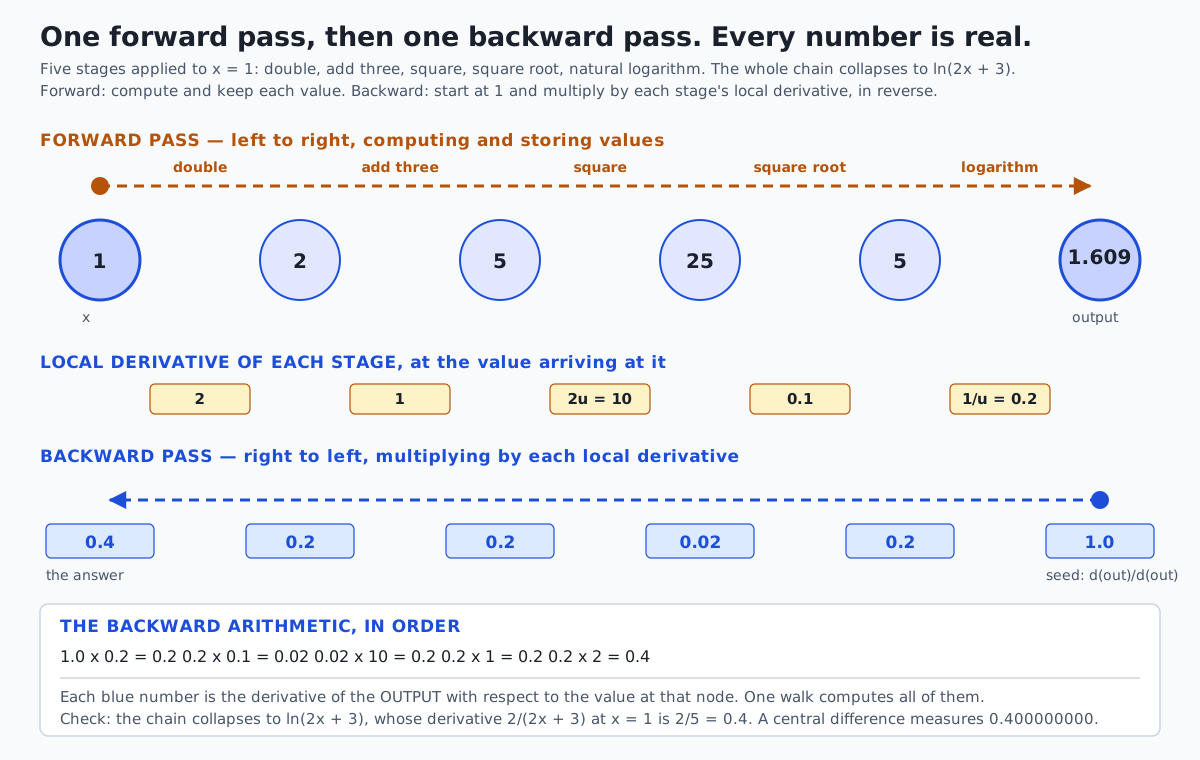
Five stages, applied left to right starting from x = 1: double, add three, square, square root, natural logarithm.
| Stage | Input | Output | Local rate at that input |
|---|---|---|---|
| double | 1 | 2 | 2 |
| add three | 2 | 5 | 1 |
| square | 5 | 25 | 2u = 10 |
| square root | 25 | 5 | 0.1 |
| logarithm | 5 | ln 5 | 1/u = 0.2 |
The derivative of the whole chain is the product: 2 × 1 × 10 × 0.1 × 0.2 = 0.4.
The column to stare at is the last one. Stage 3’s local rate is 2u, and the u it is evaluated at is 5 — the value that arrives at stage 3. Not the input x, not the final answer. Getting the evaluation point wrong is the mistake that survives longest, because the shape of the result still looks right.
Check it a completely different way. Squaring and then taking the square root of a positive number is the identity, so the five stages collapse to ln(2x + 3), whose derivative is 2/(2x + 3), which at x = 1 is 2/5 = 0.4. And a central difference of the five-stage chain measures 0.400000000. Three independent routes, one number.
What a backward pass is actually carrying
Now walk the chain from the output end, multiplying as you go. After k steps the number in your hand is the product of the last k local rates — which is exactly the gradient of the output with respect to the value arriving at that stage:
| Stage | Value in | d(output)/d(that value) |
|---|---|---|
| double | 1 | 0.4 |
| add three | 2 | 0.2 |
| square | 5 | 0.2 |
| square root | 25 | 0.02 |
| logarithm | 5 | 0.2 |
Read it upwards. The logarithm stage sees 0.2; the square-root stage sees 0.02; by the time the walk reaches the input the number is 0.4, which is the answer.
That is the entire backward pass. One walk, one multiplication per stage, every intermediate gradient computed for free on the way past — not one walk per stage. That “for free” is where the factor of a hundred billion comes from.
The part to slow down for: when paths meet, contributions add
Everything so far has multiplied. This is where addition enters, and it is the half that silently corrupts real code.
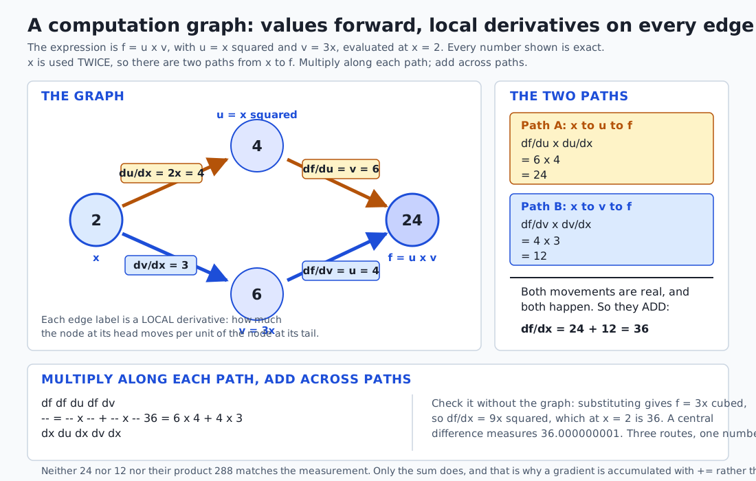
Build a small graph in which x is used twice:
u = x squared
v = 3x
f = u x v
Draw it and x has two arrows leaving it, one into u and one into v. Both end up at f.
At x = 2: u = 4, v = 6, f = 24.
Multiply the local rates along each path as usual:
path through u:   df/du x du/dx  =  v  x 2x  =  6 x 4  =  24
path through v:   df/dv x dv/dx  =  u  x 3   =  4 x 3  =  12
So — is the answer 24, is it 12, is it 24 × 12 = 288, or is it 24 + 12 = 36?
Do not reason about it. Ask the measurement. Substituting the intermediates away, the function is just f = x² · 3x = 3x³, which can be nudged directly:
| Candidate answer | Value | Matches the measurement of 36.000000001? |
|---|---|---|
| Sum of the paths, 24 + 12 | 36 | Yes |
| Path through u alone | 24 | no |
| Path through v alone | 12 | no |
| Product of the paths | 288 | no |
Only the sum survives. And it is not a convention that could have gone the other way: changing x moves the output through u and through v, both movements are real, and both happen at once. Adding them is what “both happen” means. There is no rule of nature that selects one of them as the real one, and nothing about the situation composes them.
Written honestly, without the mnemonic:
df      df   du     df   dv
--  =   -- x --  +  -- x --
dx      du   dx     dv   dx
A product for each route, a sum across routes.
Notice what this does to the cancelling reading of dy/dx = dy/du · du/dx. It has nothing to say here. There are two different intermediates and no single symbol to cancel, and the answer contains a + that no amount of symbol-shuffling produces. The mnemonic was a good mnemonic for the one-path case and it is silent on the case that actually matters for neural networks.
The computation graph
That picture generalises. Any computation is a directed graph: nodes are values, edges are operations, and every edge carries a local derivative.
The rule for the gradient of the output with respect to any node is then a single sentence:
Multiply the local derivatives along each path from that node to the output, then sum over all paths.
That sentence covers everything in this lesson. A straight chain is the special case with one path. The two-path example is the special case with two.
There is an obvious objection: the number of paths through a deep branching graph grows exponentially with depth. A ten-layer network with eight units per layer has an enormous number of paths from any early weight to the loss. Enumerating them would be hopeless.
Reverse mode never enumerates them. It gets the same answer in one sweep, by accumulating at each node instead of tracing routes. That is the algorithmic content of the whole idea, and it is why the sum-over-paths formula is the right way to understand backpropagation and the wrong way to implement it.
Forward mode and reverse mode, by cost
Both modes apply the same chain rule. They differ in which end they start from, and that decides everything.
Forward mode carries, alongside every value, its derivative with respect to one chosen input. Each operation computes both. It needs no graph and no second pass — it is genuinely simpler. The price is in the phrase “one chosen input”: a pass answers about one input only, so a function of n inputs takes n passes.
Reverse mode runs the computation forwards, storing everything, then walks backwards accumulating gradients. One forward pass plus one backward pass yields the derivative of one output with respect to every input at once, however many there are.
The choice is not about elegance. It is about the shape of the problem:
| Shape | Winner | Example |
|---|---|---|
| Many inputs, one output | Reverse mode | Training a model: millions of parameters in, one scalar loss out |
| One input, many outputs | Forward mode | Sensitivity of a whole simulation to one parameter |
| Roughly balanced | Either; forward mode is simpler | Small Jacobians |
Training is the first row, emphatically. And that is why a loss is a single number: the entire efficiency argument depends on it. If your training objective produced a thousand outputs rather than one, reverse mode would need a thousand backward passes and the economics would change.
What reverse mode pays. It has to keep the forward pass’s intermediate values alive until the backward pass consumes them, because the local derivatives are written in terms of those values — tanh’s backward step needs the tanh output, a product’s needs both its inputs. The lab measures it: a chain of fifty operations holds 101 nodes alive, and one of ten thousand operations holds 20,001. On a large model, those stored activations dominate memory use and scale with batch size and sequence length. Forward mode stores almost nothing, which is its one genuine advantage. Speed is bought with memory, and that trade is why techniques for recomputing activations instead of storing them exist at all.
Building it: reverse-mode autodiff from scratch
The engine is smaller than the explanation. A Value holds a number and a gradient, remembers which values it came from, and knows how to hand its own gradient back to them.
class Value:
    def __init__(self, data, children=(), op=""):
        self.data = float(data)
        self.grad = 0.0
        self._backward = lambda: None
        self._children = children

    def __add__(self, other):
        out = Value(self.data + other.data, (self, other), "+")

        def backward():
            # Addition passes the gradient through untouched: the local
            # rate is 1, because nudging either input by d moves the sum by d.
            self.grad += out.grad
            other.grad += out.grad

        out._backward = backward
        return out

    def __mul__(self, other):
        out = Value(self.data * other.data, (self, other), "*")

        def backward():
            # For a product, each input's local rate is the OTHER input.
            self.grad += other.data * out.grad
            other.grad += self.data * out.grad

        out._backward = backward
        return out
and the backward pass itself:
    def backward(self):
        order = topological_order(self)
        for node in order:
            node.grad = 0.0
        self.grad = 1.0                 # d(output)/d(output) = 1
        for node in reversed(order):
            node._backward()
Three things in there are worth naming.
The seed is 1.0. The derivative of the output with respect to itself is 1. That is the base case the entire chain hangs from, and every gradient in the graph is that 1 multiplied by local rates on its way back.
The order is topological, and it is not optional. Every node must appear after everything it was computed from, so that walking the list backwards guarantees a node has received every contribution owed to it before it passes any of them on. On a branching graph, an order that merely “looks right” will let a node forward its gradient early and silently drop a path. The lab’s version is iterative rather than recursive, because a chain of ten thousand operations is an ordinary graph size and would exhaust the interpreter’s stack.
Every gradient is accumulated with +=, never assigned. That single character is the multivariable chain rule. A value used in two places receives a contribution from each use, both are real, and they add.
It is worth seeing how badly that one character fails. Change += to = and the engine still runs, still returns numbers of a plausible size, and is wrong on any graph where anything is reused:
x = Value(3.0);  y = x + x;  y.backward()

     x.grad with +=   ->  2.0     correct
     x.grad with  =   ->  1.0     plausible, and wrong
Nothing raises. Nothing warns. On a straight chain with no reuse it is correct every single time, which is why the bug survives casual testing — and then it breaks on every real network, where every input feeds every hidden unit.
Add one non-linearity and the engine can build a neural network:
    def tanh(self):
        t = math.tanh(self.data)
        out = Value(t, (self,), "tanh")

        def backward():
            self.grad += (1.0 - t * t) * out.grad

        out._backward = backward
        return out
Note that the backward step reuses t from the forward pass rather than recomputing it. Every framework does this, and it is exactly why a backward pass needs the forward pass’s values in memory.
That is the whole engine. And it earns its keep immediately, in a way worth pausing on:
x = Value(3.0);  y = x * x;  y.backward()
     x.grad  ->  6.0
The engine has never heard of the power rule. It applied the product rule, added the two contributions — because x is used twice — and the power rule fell out. Every derivative rule you might have memorised is a consequence of a handful of local rates plus the chain rule, and a machine that knows only the local rates rediscovers all of them.
An everyday analogy
Keep the gear train, and let it carry the whole day.
A single gear pair is a local derivative. Two turns of A per turn of B. It is a fact about one connection, and it does not know or care what else is in the machine.
A gear train is a composition. The overall ratio is the product of the stage ratios. Add stages and you multiply more numbers; nothing about the reasoning changes. This is why a hundred-layer network is not qualitatively harder to differentiate than a one-layer network.
The forward pass is turning the input shaft and watching each gear’s position. You have to know where every gear sits, because on a real machine the ratios are not constant — the mechanism is more like a continuously variable transmission, where the ratio at each stage depends on the current position. That is the one place the analogy has to be stretched, and it is stretched deliberately, because it is exactly the fact that makes evaluation points matter.
The backward pass is asking, from the output shaft, how much each earlier shaft would have to turn. You walk back through the train multiplying ratios, and every shaft you pass gets its answer on the way. You do not walk the train once per shaft. That is reverse mode, and it is where the entire efficiency comes from.
Two gears driving the same shaft is the sum over paths. Here the analogy earns its place, because the mechanical intuition gives the right answer where the mathematical mnemonic gives none. If two gear trains both drive one output shaft, and you turn the common input, the output shaft is driven by both simultaneously. The rotations add. Nobody would suggest averaging them, or picking the larger, or multiplying them together. It is obvious in metal and it is exactly as true in the arithmetic.
A vanishing gradient is a train of reduction gears. Each stage steps the speed down slightly. One stage is unremarkable; fifty stages of ×0.9 leave the output turning at half a percent of the input speed, and fifty stages of ×0.25 leave it turning so slowly that the motion is undetectable. Nothing has broken. The machine is doing precisely what it was built to do, and the answer is useless. An exploding gradient is the same train run the other way, until something tears.
Where the analogy ends: gears are rigid and reversible, and a computation graph is neither. You cannot run a tanh backwards to recover its input, which is exactly why the forward values have to be stored. And the “ratio depends on position” stretch above is doing real work — if it were not for that, the whole business of evaluating each local rate at the right value would disappear, and with it most of the difficulty.
Examples in practice
Backpropagation through a tiny network, entirely by hand
Two inputs, two tanh hidden units, one linear output, a squared-error loss, nine parameters.
a_pre = wA1*x1 + wA2*x2 + bA        a = tanh(a_pre)
b_pre = wB1*x1 + wB2*x2 + bB        b = tanh(b_pre)
out   = vA*a + vB*b + c
loss  = (out - target) squared
The values were chosen so that every number in both passes is exact in float64. Unit A sits at a pre-activation of exactly 0, where tanh is 0 and its slope is 1. Unit B sits at exactly half the natural logarithm of 3, where tanh is exactly 0.5 and its slope is exactly 0.75. Both of those exactness claims are asserted by the lab’s test suite rather than assumed, and the choice is declared openly: it is a convenience so you can check every line with a pen, and nothing about backpropagation depends on it.
| Name | Value | Name | Value |
|---|---|---|---|
| x1 | 1 | x2 | 2 |
| wA1 | 1 | wB1 | −0.5 |
| wA2 | −0.5 | wB2 | 0.25 |
| bA | 0 | bB | ½·ln 3 |
| vA | 2 | vB | −3 |
| c | 1 | target | 1 |
Forward pass:
a_pre = 1*1 + (-0.5)*2 + 0        = 0
a     = tanh(0)                   = 0
b_pre = (-0.5)*1 + 0.25*2 + bB    = 0.5493061443
b     = tanh(bB)                  = 0.5
out   = 2*0 + (-3)*0.5 + 1        = -0.5
loss  = (-0.5 - 1) squared        = 2.25
Backward pass. Start at the end: d(loss)/d(loss) is 1. Everything else follows by multiplying.
| Step | Local rate | Gradient |
|---|---|---|
| d loss / d out | 2 × (out − target) = 2 × (−1.5) | −3 |
| d loss / d c | × 1 | −3 |
| d loss / d vA | × a = × 0 | 0 |
| d loss / d vB | × b = × 0.5 | −1.5 |
| d loss / d a | × vA = × 2 | −6 |
| d loss / d b | × vB = × (−3) | 9 |
| d loss / d a_pre | × (1 − a²) = × 1 | −6 |
| d loss / d b_pre | × (1 − b²) = × 0.75 | 6.75 |
| d loss / d wA1 | × x1 = × 1 | −6 |
| d loss / d wA2 | × x2 = × 2 | −12 |
| d loss / d bA | × 1 | −6 |
| d loss / d wB1 | × x1 = × 1 | 6.75 |
| d loss / d wB2 | × x2 = × 2 | 13.5 |
| d loss / d bB | × 1 | 6.75 |
Two rows deserve a second look.
d loss / d vA is exactly zero. Not small — zero. vA multiplies a, and a is exactly 0, so nudging vA does not move the output at all. A weight feeding a unit whose activation is zero receives no gradient and does not learn on this step. That is not a defect in the arithmetic; it is the arithmetic telling you something true about the network.
d loss / d b_pre is scaled by 0.75. That 0.75 is tanh’s slope, and it is below 1. Every tanh unit a gradient passes through multiplies it by a number in (0, 1]. Hold that thought for the next section.
And then the inputs, where two paths meet. x1 feeds both hidden units:
through unit A:  d loss/d a_pre x wA1 = -6.00 x  1.00 = -6.000
through unit B:  d loss/d b_pre x wB1 =  6.75 x -0.50 = -3.375
total:                                  -6.000 + -3.375 = -9.375
A product-only chain rule reports −6.0 here and looks entirely reasonable doing it. The lab’s test compares against a central difference — which has no opinion about which path you meant — and that settles it.
All three routes agree. The hand computation and the from-scratch engine produce identical bits on all sixteen gradients, because they perform the same multiplications in the same order on the same exact values. Central differences agree with both to within 4.5e-9. And the pass counts tell the story: reverse mode needed one sweep for all nine parameter gradients, forward mode needed nine, central differences needed eighteen.
Products that collapse and products that blow up
Take the observation that every tanh multiplies the gradient by something below 1, and run it fifty times.
| Layers | ×0.9 each | ×1.1 each |
|---|---|---|
| 1 | 9.00e−01 | 1.10e+00 |
| 10 | 3.49e−01 | 2.59e+00 |
| 30 | 4.24e−02 | 1.74e+01 |
| 50 | 5.15e−03 | 1.17e+02 |
Neither factor looks alarming. After fifty layers the shrinking chain has lost more than two orders of magnitude and the growing one has gained more than two. The early layers of the shrinking network receive a gradient a few thousandths the size of the one the last layer gets, so they learn a few thousandths as fast. They are not broken; they are slow by a factor nobody budgeted for.
Push it harder, and ask a blunt question of each result — if this were a gradient added to a weight of about 1, would the weight change at all, or would the update disappear into rounding?
| Factor | Layers | Product | Order | Lost in a weight of 1? |
|---|---|---|---|---|
| 0.9 | 200 | 7.06e−10 | −10 | no |
| 1.1 | 200 | 1.90e+08 | +8 | no |
| 0.5 | 50 | 8.88e−16 | −16 | no |
| 0.25 | 50 | 7.89e−31 | −31 | yes |
| 2.0 | 50 | 1.13e+15 | +15 | no |
The 0.5 row contradicts the obvious guess, and it is worth getting right. 0.5⁵⁰ is about 8.88e-16 and float64’s epsilon is about 2.22e-16, so it looks as though adding it to 1.0 should lose it. It does not: 8.88e-16 is exactly four epsilons — four representable gaps — and four gaps is still four gaps. It takes three more halvings, to 0.5⁵³ = half an epsilon, before the addition rounds away to nothing. The lab asserts both halves of that.
The row that genuinely vanishes is 0.25⁵⁰, and 0.25 was not chosen for drama. It is the largest slope the sigmoid ever has, measured earlier in this very lesson. A stack of sigmoid layers is multiplying numbers no bigger than that one, and this is the concrete arithmetic reason deep networks were hard to train before the fixes the course reaches later.
The measurement that corrects the story
Everything in that last section multiplied a constant factor. Real layers do not work that way, and the difference turns out to matter enormously.
Stack forty real tanh operations and measure the gradient:
| Depth | Gradient at x = 0.9 | Ratio to the row above |
|---|---|---|
| 1 | 4.869174e−01 | — |
| 5 | 1.255802e−01 | 3.877 |
| 20 | 2.213240e−02 | 2.492 |
| 40 | 8.397332e−03 | 2.636 |
| 160 | 1.113159e−03 | 2.771 |
Now the naive prediction. tanh’s slope at the input is about 0.487, so forty tanh layers “should” multiply the gradient by that forty times over:
0.486917 ** 40      = 3.149274e-13     the prediction
measured at depth 40 = 8.397332e-03     the measurement
Ten orders of magnitude apart. The prediction is not slightly off; it is wrong in kind.
The reason is worth more than the number. Each tanh pulls its input closer to 0, and tanh’s slope at 0 is 1. So the deeper the stack goes, the closer every local rate creeps back towards 1, and the product decays like a power of the depth rather than exponentially. You can see it in the ratio column, which settles near 2.8 per doubling of depth instead of growing.
A product of constants is the wrong model for a product of rates that depend on where they are evaluated. The previous section is still the right picture of what a chain of fixed factors does — and a weight matrix that is consistently too small or too large really does behave that way, which the lab confirms by showing a genuinely constant 0.487 collapsing below 1e-12 in the same forty steps. But “tanh saturates, therefore gradients vanish” is a claim that has to be measured on the network in front of you, not deduced from the shape of the curve.
This measurement was not planned. It came out of a test written to confirm the textbook story, which failed. The test was rewritten to assert what is true — a monotonic fall, a gap of more than nine orders against the prediction, and the contrast case where a constant factor does collapse — rather than what was expected.
Implications: security, privacy, performance, scalability, and cost
Performance. The headline number is the one this lesson opened with: reverse mode computes every input derivative in roughly the cost of two forward passes, regardless of how many inputs there are. The measured pass counts on a 25-input function are 1, 25 and 50 for reverse mode, forward mode and central differences respectively — and the first two produce bit-identical answers. The practical rule is that a backward pass costs roughly one to two times a forward pass, so training a model costs about three times what running it costs. That ratio holds across architectures because it follows from the structure of the rule, not from any particular network.
Scalability and memory. The cost that scales badly is memory, not time. Every intermediate value from the forward pass must survive until the backward pass consumes it. Activation memory grows with model depth, batch size and — for sequence models — sequence length, and on large models it dominates. This is why gradient checkpointing exists: throw away some stored activations and recompute them during the backward pass, trading time for memory. It is a direct consequence of what reverse mode needs, and you can predict that the trade exists purely from understanding the algorithm.
Cost. Compute is billed by the hour. The three-times-inference figure above is roughly what a training budget is built on, and the memory ceiling is what decides which hardware you need, which is usually the larger line item. A batch size that does not fit is not a performance problem; it is a procurement problem.
Numerical robustness. Long products leave the useful float range quickly and quietly, in both directions. Underflow gives exactly zero and no warning; overflow gives inf, after which a single further operation turns parameters into nan and the run is dead — often thousands of steps after the actual cause. A training loop that does not check its own loss for finiteness will happily spend hours computing with nan. Gradient clipping is partly a numerical guard rather than only an optimisation heuristic.
Security. Two points, both real.
The first is a bug class rather than an attack. A silently wrong gradient — the =-instead-of-+= bug is the model case — produces code with correct types, correct shapes, plausible magnitudes and wrong answers, and nothing raises. A wrong gradient still has some correlation with the right one, so the loss even goes down for a while. In a system where the trained model makes decisions about people, “it seemed to be training” is not evidence that it trained correctly. The only defence is the one this lab uses throughout: check the analytic result against an independent numerical one that shares none of its assumptions. That is what gradient checking is, and it is cheap to run once.
The second is availability. Because reverse mode’s memory scales with input size, anything that differentiates over user-controlled input length has a memory bound that must be set explicitly rather than discovered. An input that is merely large, with no malice involved, can exhaust the host.
Privacy. Gradients are not anonymous summaries of training data. A gradient is computed from specific examples and carries information about them — which is the entire basis of the federated-learning threat model, where gradients rather than data are shared and can leak the data anyway. This lesson does not develop that, but it is worth knowing that the quantity you are learning to compute is derived from the input in a way that is not one-directional in practice, and that treating shared gradients as if they were aggregate statistics is a mistake with a literature behind it.
Alternatives: free, open source, and commercial
There are four ways to get a derivative out of a computer, and it is worth being clear that they are genuinely different methods rather than variations on one.
| Approach | What it does | Exact? | Cost for n inputs, 1 output |
|---|---|---|---|
| Numerical (finite differences) | Nudges the input and watches the output | No — truncation and rounding error | 2n full evaluations |
| Symbolic | Manipulates the formula, returns a formula | Yes | Can grow explosively in expression size |
| Forward-mode automatic | Propagates derivatives with the values | Yes, to float rounding | n passes |
| Reverse-mode automatic | Propagates derivatives backwards from the output | Yes, to float rounding | 1 pass |
Honesty note before the tool list: of the tools below, only the from-scratch engine and the numerical checking tool were actually run for this lesson. PyTorch, JAX, TensorFlow and SymPy are not installed in this environment and no output from any of them is reproduced anywhere in this lesson or its lab. What follows is described from their documentation, and it is described as design rather than as measurement.
The engine you build here. Free, and the only one in this list you will have written. Choose it when the goal is understanding, when you need something with no dependencies, or when you want to be able to read a real framework’s source and recognise what it is doing. Its concrete example is the seventy-line Value class in the lab, checked against central differences on every gradient. Its limitation is engineering, not concept: it is scalar-only, pure Python, and has no fused operations or hardware acceleration, so it is thousands of times slower than a real framework on real work. That difference is entirely in the engineering. Nothing about the idea changes when the numbers become tensors.
Numerical differentiation — Day 108’s central difference, standard library only, free. Choose it as a checking tool, never a production one, and that distinction is the whole point of including it. Its concrete example is every verification in this lab: an independent measurement that knows nothing about the graph, which is exactly what makes it a valid check on an analytic gradient. Use it to validate a hand-derived gradient or a custom autodiff operation; do not use it to train anything, because it is approximate and costs 2n evaluations.
PyTorch autograd — free and open source, with paid managed platforms available from various vendors for running it at scale. According to its documentation it builds a dynamic computation graph as operations execute and provides tensor.backward() to run reverse-mode differentiation over it; tensors record gradients when created with requires_grad=True. Choose it for research and for anything where the model structure changes at runtime, since the graph is rebuilt each forward pass. The shape of use is loss.backward() followed by reading .grad off each parameter — which is, deliberately, the same shape as the engine you are about to write.
JAX grad — free and open source. Its documentation describes a functional approach: grad(f) returns a new function that computes the gradient of f, and transformations compose, so grad(grad(f)) gives a second derivative and jit(grad(f)) compiles it. Choose it when you want function transformations to compose cleanly, when you need higher-order derivatives without special handling, or when compilation to accelerators matters. It also exposes forward mode explicitly, which most frameworks do not, and that makes it the natural place to experiment with the trade this lesson describes.
TensorFlow GradientTape — free and open source. Its documentation describes recording operations onto a “tape” within a context manager and then calling tape.gradient(target, sources). Choose it if you are already in the TensorFlow ecosystem or need its deployment tooling. The explicit tape makes the record-then-replay structure of reverse mode unusually visible, which is pedagogically nice: the tape is the topological order this lesson’s engine computes.
SymPy — free and open source, and a genuinely different thing. It differentiates formulas symbolically and hands back a formula you can read, simplify or evaluate anywhere. Choose it when you want to see the derivative rather than evaluate it — deriving a result by hand and checking your algebra, or generating code for a closed-form expression. Do not choose it for a neural network: symbolic differentiation of a deeply nested expression can produce an expression far larger than the original, which is precisely the failure mode automatic differentiation avoids by never building the formula at all.
The honest summary is that for training a model there is no real competition — reverse-mode automatic differentiation wins on cost and exactness together, and every major framework implements it. The interesting choice is not whether to use it but which of numerical, symbolic and automatic differentiation belongs at which point in your workflow: symbolic for deriving, numerical for checking, automatic for running.
Comparison with related concepts
The chain rule and the product rule. The product rule handles two functions multiplied; the chain rule handles two functions composed. They are different rules and they travel together — the engine’s __mul__ implements the product rule and its graph walk implements the chain rule, and the pair is enough to differentiate any polynomial. Notably, you do not need the power rule at all: the engine rediscovers it from x * x, because x is used twice and the two contributions add.
The chain rule and the gradient (Day 109). A gradient collects partial derivatives. The chain rule tells you how to compute each one when the variable is buried. Day 109’s gradient of a two-variable function was computed directly; today’s is computed by chaining through intermediates, and the multivariable chain rule is what makes the second possible. Day 109 also established that the gradient points uphill and is perpendicular to the contour — properties of the vector, unaffected by how you obtained it.
Backpropagation and reverse-mode differentiation. These are the same algorithm. Backpropagation is the name the neural-network community gave to reverse-mode automatic differentiation applied to a network’s computation graph. If a text presents them as different things, it is drawing a distinction that does not exist.
Backpropagation and gradient descent. Constantly confused, entirely separate. Backpropagation computes gradients. Gradient descent uses them to update parameters. You can compute gradients and do something else with them entirely, and you can do gradient descent with gradients obtained some other way. Day 111 is the second one.
Automatic differentiation and numerical differentiation. Not related in method, despite both producing numbers. Numerical differentiation samples the function at nearby points and has the two error terms Day 108 measured. Automatic differentiation applies exact local derivatives to the operations the program performs. The lab’s comparison is deliberately structured around this: two analytic routes are compared with == or a tolerance of 1e-12, while an analytic route against a measured one gets 1e-6. That million-fold gap is not sloppiness — it is the honest size of a central difference’s own error.
Forward mode and reverse mode. The same rule from opposite ends. Forward mode is simpler and stores nothing; reverse mode needs a graph and stored activations. The choice is decided entirely by the ratio of inputs to outputs.
Vanishing gradients and dead units. Related and distinct. A vanishing gradient is a product that has collapsed across many layers. A dead unit is a single local rate that is zero — like d loss/d vA in this lesson’s network, which is exactly zero because it multiplies an activation of zero. The first is a depth problem; the second is a one-node problem that no amount of shallowness fixes.
When to use it — and when not to
Use the chain rule whenever a quantity you care about depends on a quantity you can change through one or more intermediate steps. That is every neural network, and also every sensitivity analysis, every physical model with derived quantities, and a great deal of ordinary calculation that nobody labels as calculus.
Use reverse-mode automatic differentiation when you have many inputs and one scalar output. Training is the canonical case. If you are writing a training loop, this is not a choice; it is the only affordable option.
Use forward mode when the ratio is the other way round — one or a few inputs, many outputs. Sensitivity of a whole simulation to a single parameter is the classic example. It is also simpler to implement and needs no stored graph, so for a small number of inputs it can be the better engineering choice even where reverse mode would work.
Use numerical differentiation to check, essentially never to run. It is the independent measurement that catches an analytic mistake, and every custom gradient you write should be checked against it once. Its cost and its error both rule it out for production.
Use symbolic differentiation when you want to look at the derivative rather than evaluate it — verifying algebra, deriving a closed form, generating code for a simple expression.
Do not reach for the chain rule when the composition collapses to something you can differentiate directly. This lesson’s five-stage chain collapses to ln(2x + 3); differentiating that takes one step instead of five. Recognising the collapse is a skill, and it is also a free check — two routes to one number, which is how the lab verifies that chain in the first place.
Do not use a numerical gradient inside a training loop, however tempting it is for a small model. It is 2n evaluations per step and it is approximate. If you find yourself doing this, you have re-derived the problem that reverse mode exists to solve.
Do not assume the vanishing-gradient story without measuring it. This lesson’s own measurement contradicted the standard argument by ten orders of magnitude on a stack of tanh layers. The reasoning that fails is easy to state and easy to believe: take a representative local rate, raise it to the power of the depth. It fails because local rates are not constant, and the forward pass moves the point at which they are evaluated. When you need to know whether a particular network has a gradient problem, measure that network.
And do not write a gradient by hand without checking it. Not because hand derivation is hard, but because a wrong gradient does not announce itself. It has the right type, the right shape and a plausible magnitude, and the loss goes down for a while.
Knowledge check
Eight questions accompany this lesson, covering the gear intuition, the evaluation-point mistake, why contributions sum over paths, what a backward pass carries, why reverse mode wins when there are many parameters, the += bug and its silence, the stacked-tanh measurement that corrects the standard story, and why an analytic-against-numerical comparison needs a looser tolerance than an analytic-against-analytic one.
Two are worth attempting before you read anything else: the one asking what happens when a variable reaches the output by two routes, and the one asking why reverse mode wins. Those are the two facts that everything else today rests on.
Hands-on exercise
The lab is “Rates Multiply”, and its centrepiece is a working reverse-mode automatic differentiation engine that you write.
cd labs/sections/math-statistics-and-data/day-110-the-chain-rule
python3 -m venv .venv
.venv/bin/pip install -r requirements/requirements.txt
Nine exercises, in order. Fourteen plumbing functions in starter/chainrule.py; the Value engine and the Dual forward-mode class in starter/autodiff.py; the three pass-counting wrappers that make the cost comparison concrete; the two-layer network backpropagated by hand in starter/network.py; and forty-two predictions in starter/answers.py that you should fill in before running anything.
Check yourself as you go:
.venv/bin/pytest starter -qUnattempted work is reported as skipped, never as failed. Wrong work fails with your answer printed beside the correct one.
Expected output
An untouched checkout:
2 passed, 163 skippedA finished one:
165 passedThe full harness ends with:
120 checks, 0 failure(s).and exits 0. Along the way, the four candidate answers put to a measurement:
     candidate answer            value      matches the measurement?
     ------------------------------------------------------------
     sum of the paths, 24 + 12   36         YES
     path through u alone        24         no
     path through v alone        12         no
     product of the paths        288        no
and the engine rediscovering a rule nobody told it:
      x = 3,  y = x x x
      y.data = 9.0,  x.grad = 6.0   <- 2x, the power rule
Validate your work
bash tests/run_tests.sh; echo "exit=$?"prints120 checks, 0 failure(s).andexit=0..venv/bin/pytest examples -q -p no:cacheproviderprints235 passed..venv/bin/pytest starter -q -p no:cacheproviderprints165 passedwhen you are finished.- Each of the seven reference scripts ends with
every assertion held. - Your
hand_gradients()and yourengine_gradients()agree exactly on all sixteen network gradients — not approximately. If they do not, one of them is doing the arithmetic in a different order.
Troubleshooting
ModuleNotFoundError on chainrule means you ran a reference script from the lab directory rather than from inside examples/; they import their neighbours from beside themselves.
Tests that keep skipping after you have written code usually mean a leftover return None survived below your implementation — several skeletons put it on the last line of a long docstring.
A RecursionError on a deep graph means your topological_order is recursive. Ten thousand operations is an ordinary graph size and there is a test that builds exactly that.
A gradient of 1.0 where you expect 2.0, or 3.0 where you expect 6.0, is the =-instead-of-+= bug. It only shows up when a value is reused, which is why x + x and x * x are the two tests that catch it.
A numerical gradient that disagrees with your engine in the eighth decimal place is correct behaviour, not a bug. Do not tighten the tolerance; you would only be rediscovering Day 108.
troubleshooting.md covers all of these in full, along with why the harness clears bytecode caches at the start of its run — the README tells you to run pytest starter -q, that command legitimately writes __pycache__ and .pytest_cache, and an earlier version of the harness would then have failed you for following the instructions.
Common mistakes
- Evaluating the outer derivative at
xinstead of atu. Gives 12 where the answer is 42, and looks entirely reasonable. - Taking one path and stopping. Gives
−6.0ford loss/d x1where the answer is−9.375. This is the day’s most instructive failure, and the harness’s deliberate self-test uses exactly this wrong value to prove it can detect a failure at all. - Assigning a gradient instead of accumulating it. Runs, looks fine, silently wrong on every graph with a reused value.
- Dividing a central difference by
hinstead of2h. Produces a clean factor of two, which is easy to mistake for a units problem. - Writing a recursive topological sort. Correct on small graphs, fails on real ones.
- Widening a tolerance until a test passes. A tolerance chosen that way is a tolerance chosen by whatever bug happened to exist at the time. Every tolerance in this lab is derived in
dataset.pyfrom the error terms that govern its comparison, with the arithmetic written out beside it, and a test asserts that none of them is loose enough to be meaningless.
Practice assignment
Extend the engine and use it to check something you did not write.
- Add
exp()to yourValueclass. The derivative ofeˣiseˣ, so the backward step can reuse the forward value exactly astanhdoes. Verify it against a central difference at three points. - Build the sigmoid out of your own operations — you will need a reciprocal as well — and measure its slope at zero with your engine. Confirm you get
0.25, and then confirm by scanning a range that no other point gives more. - Re-derive three rules you may have memorised. Using only
+,×and your engine, compute the derivative ofx³, of(x + 1)(x + 2)and ofx²·x³at a point of your choosing. Check each against a central difference. Then write one paragraph on what the engine had to know in order to get them right, and what it did not. - Backpropagate a three-layer network by hand. Add one more hidden layer to the lab’s network, choose your own values, and compute every gradient twice — by hand and with your engine. Count the paths from each input to the loss before you start, and see whether your hand method scales the way you expected.
- Write the gradient-check function you should have been using all along. Given any function and a point, it should return the analytic gradient, the numerical gradient, and the largest relative disagreement. Justify the tolerance you compare against, in a comment, from the error terms rather than from what happened to pass.
Extension challenge
Three, in increasing order of difficulty.
Make the bug visible, then predict its damage. Change one += to = in your engine and run the reference suite. Record which tests fail, which still pass, and how large the wrong answers are. Then — before running anything — predict whether the two-layer network’s loss would still go down under gradient descent using those corrupted gradients, and by how much less than it should. Day 111 gives you the loop to find out whether you were right. This is the most valuable exercise on this page, because it teaches you what a silent numerical bug feels like from the inside.
Count the paths, then explain why nobody does. Write a function that enumerates every distinct path from a given leaf to the output of a Value graph and verifies that the sum of the path products equals the gradient your engine computed in one sweep. Confirm it on the two-layer network, where x1 has two paths. Then extend the network to three layers and count again, work out the general formula for a network with L layers and k units per layer, and evaluate it for L = 10, k = 8. Write down both numbers — the path count and the number of multiplications reverse mode actually performed — side by side.
Find your own vanishing point, and beat the prediction. The lesson measured stacked tanh. Repeat the experiment for the sigmoid, and for tanh interleaved with a multiplication by 0.5, and find the depth at which each gradient first stops moving a weight of 1.0. Predict the ordering before you measure. Then explain any case where you were wrong — the reasoning in the lab’s section 6 is the tool for that, and the honest answer for at least one of these cases is that the constant-factor model does not apply.
The AI thread. Backpropagation is the chain rule applied to a computation graph, computed in reverse. That is the whole of it — there is nothing more exotic underneath, no separate theory, no additional idea that arrives later in the course to complete the picture. When PyTorch runs loss.backward(), it walks the graph your forward pass built, in reverse topological order, multiplying by local derivatives and accumulating with += at every node. You have now written that, and the difference between your seventy lines and the real thing is tensors, fused kernels, hardware dispatch and memory planning — engineering, all of it, and none of it conceptual.
Two consequences are worth carrying forward. The first is that the thing making training affordable is not the chain rule itself but its direction: one backward pass yields every parameter’s gradient because a scalar loss lets the shared work be computed once. Every architectural decision in deep learning inherits that constraint, starting with the fact that a training objective is one number. The second is that the failure modes you met today — a product collapsing to 7.9e-31, a product exploding to inf, a += silently becoming = — are the failure modes of production training runs, not toy problems. The techniques the course reaches later are responses to them, and you now know what they are responding to.
Tomorrow, Day 111, you take the gradients this day produces and write the loop that follows them downhill. The gradient tells you which way is down; gradient descent decides how far to step. That loop is short, and it will work, and you will know exactly why.
Quiz
Q1. Gear A turns twice for every turn of gear B, and gear B turns three times for every turn of gear C. How many times does A turn per turn of C, and what does that have to do with calculus?
- Five, because the rates add — and the chain rule likewise adds derivatives along a chain
- Six, because the rates multiply — and that is the chain rule, with the notation removed
- Two thirds, because the rates divide — and the chain rule is a quotient of derivatives
- It cannot be determined without knowing the tooth counts, and the chain rule likewise needs the underlying functions
Show answer
Answer: B. Six, because the rates multiply — and that is the chain rule, with the notation removed
Turn C once and B turns three times; each of those three turns spins A twice; so A turns six times. The rates multiplied, and nothing about that reasoning required calculus — "per" stacks by multiplying. That is exactly the chain rule: dA/dC = dA/dB x dB/dC = 2 x 3 = 6. Option 3 is the closest to a real objection and is still wrong: the ratios ARE the tooth counts, already expressed as rates, which is all the rule needs. The one thing calculus adds is that a derivative, unlike a gear ratio, can depend on where you are — which is why every local rate has to be evaluated at the value that actually arrives at its stage.
Q2. For y = (3x + 1)² at x = 2, a reader computes 2 x 2 x 3 = 12. The correct answer is 42. What went wrong?
- The outer derivative was evaluated at x rather than at u = 3x + 1, which is 7 there
- The inner derivative was omitted, and 12 is what you get from the outer rate alone
- The power rule does not apply to a composition, so a different rule was needed
- The two derivatives should have been added rather than multiplied
Show answer
Answer: A. The outer derivative was evaluated at x rather than at u = 3x + 1, which is 7 there
The outer function is f(u) = u², whose derivative is 2u — and the u it must be evaluated at is the value that arrives from the inner function, which is 3(2) + 1 = 7. So the correct product is 2 x 7 x 3 = 42, while evaluating 2u at x = 2 gives 2 x 2 x 3 = 12. This is the single most durable mistake in the topic, because the wrong answer still has the right shape: it is a product of two plausible numbers, and nothing about it looks like an error. The lab asserts the mistake as a mistake — a test checks that 12 and 42 differ — so that no future edit can quietly make the wrong route correct. Option 1 describes a different error that happens to be arithmetically close here and would give 14, not 12.
Q3. A variable x reaches an output f through two separate routes: once via u = x², once via v = 3x, with f = u x v. At x = 2 the path products are 24 and 12. What is df/dx?
- 24, because the path through u carries the larger contribution and dominates
- 288, because the two paths compose and their contributions multiply
- 36, because both movements are real and both happen, so the contributions add
- 18, the average of the two paths, since x cannot move through both at once
Show answer
Answer: C. 36, because both movements are real and both happen, so the contributions add
Substituting the intermediates gives f = x² x 3x = 3x³, so df/dx = 9x², which at x = 2 is 36 — and a central difference, which has no opinion about rules, measures 36.000000001. The lab puts all four candidates to that measurement and only the sum survives. The reasoning behind the sum is worth more than the check: nudging x moves the output through u AND through v, both movements genuinely occur, and adding them is precisely what "both happen" means. There is no rule of nature selecting one path as the real one, and nothing about the situation composes the paths, so options 0 and 1 have no mechanism behind them. Option 3 is the most seductive because it feels like conservation — but x does move through both routes at once, and averaging would understate the true rate by half. This is also why an autodiff engine accumulates gradients with += rather than assigning them: assignment is exactly the bug of letting the last path overwrite the others.
Q4. A five-stage chain has local rates 2, 1, 10, 0.1 and 0.2, evaluated at x = 1. During a backward pass, what is the number being carried after the walk has passed the last two stages?
- 0.4, the derivative of the whole chain, since the walk always carries the final answer
- 0.3, the sum of the last two local rates
- 0.02, the product of the last two local rates
- 0.1, the smaller of the two rates, since the chain is limited by its weakest stage
Show answer
Answer: C. 0.02, the product of the last two local rates
After k steps from the output end, the backward pass is carrying the product of the last k local rates — here 0.2 x 0.1 = 0.02. That number is not an intermediate curiosity: it is the gradient of the output with respect to the value arriving at that stage, computed for free on the way past. Continue the walk and it becomes 0.02 x 10 = 0.2, then 0.2 x 1 = 0.2, then 0.2 x 2 = 0.4, which is the derivative of the whole chain — confirmed independently by collapsing the five stages to ln(2x + 3), whose derivative 2/(2x + 3) at x = 1 is 2/5. Option 0 describes only the final step. Option 3 invokes a bottleneck intuition that does not apply — a product is not governed by its smallest factor, as the 10 in the middle of this chain demonstrates by pulling the running value back up.
Q5. Why does reverse-mode differentiation win when a model has many parameters and a single scalar loss?
- It is more numerically accurate than forward mode, which accumulates rounding error over the chain
- It needs one forward-and-backward sweep to obtain every input gradient, while forward mode needs one complete run per input
- It avoids storing intermediate values, so it uses far less memory on a deep network
- It computes an approximate gradient, which is cheaper and good enough for training
Show answer
Answer: B. It needs one forward-and-backward sweep to obtain every input gradient, while forward mode needs one complete run per input
Both modes apply the same chain rule and both are exact up to float rounding; they differ only in which end they start from, and that decides the cost. Forward mode carries derivatives with respect to ONE seeded input, so a function of n inputs takes n runs — the lab measures 1, 25 and 50 passes for reverse mode, forward mode and central differences on a 25-input function, and all three produce the same gradients. Scale that to a hundred million parameters and one loss and the ratio is a hundred million to one; that asymmetry is the entire economic basis of modern training. Option 0 is false — the lab asserts the two modes agree to the last bits. Option 3 is false and matters: reverse mode is exact, unlike the finite differences used to check it. Option 2 inverts the truth, and the inversion is the honest caveat: reverse mode must keep every forward value alive until the backward pass consumes it, because the local derivatives are written in terms of those values. Forward mode is the one that stores almost nothing. Speed is bought with memory, which is why activation memory dominates on large models.
Q6. In an autodiff engine, a developer writes `self.grad = out.grad` instead of `self.grad += out.grad` in every backward step. What happens?
- Every gradient becomes zero, because the seed is overwritten before it propagates
- The engine raises an error the first time a value is reused, since a gradient would be written twice
- The engine runs, returns plausible numbers, and is wrong on any graph where a value is used more than once
- Nothing changes, since each node receives its gradient exactly once in a correct topological order
Show answer
Answer: C. The engine runs, returns plausible numbers, and is wrong on any graph where a value is used more than once
It runs. Nothing raises and nothing warns. On a straight chain with no reuse it is correct every time, which is why the bug survives casual testing. It breaks the moment a value feeds more than one operation: the second contribution overwrites the first instead of adding to it, and the node ends up reporting one path where it owed the sum of several. With x = 3 and y = x + x, the correct gradient is 2 and the assigning version gives 1 — a number that is the right type, the right shape and the right order of magnitude. This is the chain rule sum-over-paths fact compressed into one character, and it is the model case for the most expensive class of numerical bug: correct types, plausible magnitudes, wrong answers, no signal. Option 3 misunderstands what topological order guarantees — it fixes the ORDER of arrival so that nothing propagates early, but it cannot make several arrivals into one.
Q7. A chain of 50 factors, each 0.9, gives about 5.15e-3, and 50 factors of 1.1 give about 117. A reader concludes that stacking 40 tanh layers, whose slope at the input is about 0.487, will give a gradient near 0.487⁴⁰ = 3.1e-13. Measurement gives 8.4e-3. Why?
- Floating-point rounding accumulates over 40 multiplications and inflates the result
- The local rates are not constant: each tanh pulls its input towards zero, where tanh has slope 1, so the rates climb back towards 1 as the stack deepens
- The measurement is wrong, because a central difference is unreliable at this magnitude
- tanh is not differentiable everywhere, so the chain rule does not strictly apply to a deep stack
Show answer
Answer: B. The local rates are not constant: each tanh pulls its input towards zero, where tanh has slope 1, so the rates climb back towards 1 as the stack deepens
The prediction is out by ten orders of magnitude, and the cause is a modelling error rather than an arithmetic one. A product of CONSTANTS decays exponentially, and the lab asserts exactly that for a fixed factor of 0.487, which does fall below 1e-12 in forty steps. But a local rate depends on where it is evaluated, and the forward pass moves that point: each tanh maps its input closer to zero, tanh has slope 1 at zero, so successive local rates creep back towards 1 and the product decays like a power of the depth instead. The measured ratio settles near 2.8 per doubling of depth rather than growing. This is why the lab asserts the shape — a monotonic fall and a gap of more than nine orders against the prediction — rather than the value, and why "tanh saturates, therefore gradients vanish" is a claim that has to be measured on the network in front of you. Option 0 is the wrong scale entirely; rounding over 40 operations moves the last digits, not the exponent.
Q8. The lab compares a hand-worked gradient against its autodiff engine with `==`, but compares both against a central difference with a tolerance of 1e-6. Why the different standards?
- The engine is trusted more than the hand computation, so it is held to a stricter standard
- Exact comparison is only valid for integers, and the numerical gradient happens to be fractional
- A tolerance of 1e-6 would be too slow to evaluate at exact precision, so it is used only where speed matters
- The first pair performs the same multiplications on the same exact values, while a central difference is an approximation with truncation and rounding error of its own
Show answer
Answer: D. The first pair performs the same multiplications on the same exact values, while a central difference is an approximation with truncation and rounding error of its own
These are two different kinds of comparison and using one tolerance for both would misrepresent one of them. The hand computation and the engine multiply the same exact float64 quantities in the same order, so they agree bit for bit — and the network in this lab was deliberately built so every quantity is exact, which is what the bias of half the natural logarithm of 3 buys: tanh returns exactly 0.5 there and 1 minus tanh squared is exactly 0.75. Anything looser than equality would be hiding a bug. A central difference, by contrast, carries truncation error of about (h²/6)|f‴| and rounding error of about EPSILON|f|/h; at h = 1e-5 that bound is roughly 9.7e-9 here, so 1e-6 is a justified tolerance with about a hundredfold margin, and the measured worst gap was 4.5e-9. Tightening it to 1e-12 would fail on correct code for reasons that have nothing to do with the chain rule; loosening the analytic comparison to 1e-6 would pass code that had dropped an entire path.
Glossary
- Composition
- Feeding the output of one function into another, written f(g(x)) and read from the inside out: g runs first on x, and f runs on whatever g returned. Composition is not commutative — at x = 2, squaring 3x + 1 gives 49 while tripling x squared and adding one gives 13.
- Chain rule
- The rule that the derivative of a composition is the product of the local rates along it: dy/dx = dy/du x du/dx, where u = g(x). The outer derivative is evaluated at the inner value u, never at x. Stated without notation: if A changes twice as fast as B and B changes three times as fast as C, then A changes six times as fast as C.
- Local derivative
- The derivative of a single operation with respect to one of its own inputs, evaluated at the value that actually arrives at that operation. For a product the local derivative with respect to one factor is the other factor; for tanh it is 1 minus tanh squared; for an addition it is 1. The chain rule multiplies local derivatives, so getting the evaluation point wrong corrupts the whole product.
- Computation graph
- A directed graph whose nodes are values and whose edges are operations, built as an expression is evaluated. Each edge carries a local derivative. The gradient of the output with respect to any node is the sum, over every path from that node to the output, of the product of the local derivatives along that path.
- Node
- One value in a computation graph, together with the record of which values it was computed from. In the engine built in this lab a node is a Value object holding a number, a gradient, a tuple of children, and a small function that hands its gradient back to those children.
- Path
- One route from a node to the output through the computation graph. A variable used more than once has more than one path, and its gradient is the sum of the path products. Reverse-mode differentiation never enumerates paths — it gets the same answer in one sweep, which is what makes it affordable on a graph where the number of paths grows exponentially with depth.
- Forward pass
- Running a computation from inputs to output, computing and storing every intermediate value. The stored values are not optional bookkeeping: the local derivatives are written in terms of them, so a backward pass cannot run without them.
- Backward pass
- Walking the computation graph from the output back towards the inputs, multiplying by each local derivative and accumulating the result at every node. After k steps the number being carried is the product of the last k local rates, which is exactly the gradient of the output with respect to the value at that point in the chain.
- Reverse-mode differentiation
- Applying the chain rule from the output backwards. One forward pass plus one backward pass yields the derivative of a single output with respect to every input at once, no matter how many inputs there are. It is what makes training practical, and it pays for that speed by keeping the forward pass values in memory.
- Forward-mode differentiation
- Applying the chain rule from the inputs forwards, carrying each value alongside its derivative with respect to one chosen input. It needs no graph and no second pass, but answers about one input per run — so a function of n inputs costs n runs. It wins in the opposite shape from reverse mode: one input, many outputs.
- Dual number
- A pair holding a value and its derivative with respect to a seeded input, with arithmetic defined so that the derivative propagates automatically — addition adds both parts, multiplication applies the product rule. Dual numbers are the whole implementation of forward mode.
- Automatic differentiation
- Computing exact derivatives by applying the chain rule to the operations a program actually performs. It is neither symbolic differentiation, which manipulates formulas and can blow up in size, nor numerical differentiation, which approximates with finite differences and carries truncation and rounding error. Automatic differentiation is exact up to float rounding and costs a small constant factor over the original computation.
- Backpropagation
- Reverse-mode automatic differentiation applied to a neural network: build the computation graph during the forward pass, seed the loss gradient with 1, and walk backwards applying the chain rule to get every parameter gradient in one sweep. It is not a separate algorithm from the chain rule — it is the chain rule with a schedule.
- Gradient accumulation
- Adding each incoming contribution to a node gradient rather than overwriting it, written += rather than = in a backward step. This one character implements the multivariable chain rule: a value used in several places receives a contribution from each use, and all of them are real. Assignment instead produces code that runs, looks reasonable and is wrong on every graph containing a reused value.
- Vanishing gradient
- A gradient that becomes too small to move a weight, because the product of many local rates below 1 collapses towards zero. Fifty factors of 0.25 — the sigmoid maximum slope — give about 7.9e-31, which changes a weight of 1 not at all. The arithmetic is correct; the answer is useless, and those are different complaints.
- Exploding gradient
- The mirror image: a product of many local rates above 1 growing without bound. Fifty factors of 1.1 give about 117 and two hundred give about 1.9e+8. Nothing raises an exception on the way; a large enough product silently becomes inf, after which one more operation turns every parameter into nan.
- Squared-error loss
- A single number measuring how wrong a prediction is, computed as (prediction minus target) squared. Its derivative with respect to the prediction is 2 times (prediction minus target), which is where every backward pass in this lesson begins. Squaring makes the loss a scalar with a well-defined minimum, and being a scalar is what lets reverse mode differentiate it against millions of parameters in one sweep.
- Topological order
- An ordering of a computation graph in which every node appears after everything it was computed from. A backward pass must visit that order in reverse, so that no node passes its gradient onwards before it has received every contribution owed to it. On a branching graph any convenient order will silently drop a path.
- Saturation
- The region where a bounded non-linearity flattens out and its local derivative approaches zero — tanh far from the origin, or the sigmoid at either extreme. Saturation is the usual explanation for vanishing gradients, but it is a claim about a particular network at particular values rather than a property of the curve: a stack of pure tanh operations pulls its own inputs back towards zero, where the slope is 1, and decays far more slowly than a constant-factor argument predicts.
Sources and further reading
- Chain rule — Wikipedia (accessed 2026-08-17)
- Automatic differentiation — Wikipedia (accessed 2026-08-17)
- Derivative — Wikipedia (accessed 2026-08-17)
- NumPy documentation — NumPy Developers (accessed 2026-08-17)
- Essence of calculus — 3Blue1Brown (accessed 2026-08-17)
- Single Variable Calculus, Fall 2006 (18.01) — MIT OpenCourseWare (accessed 2026-08-17)
Kept in this browser, no account needed. Your progress page turns the whole record into one link you can bookmark or open on another device.