Math, Statistics, and Data › Probability and Statistics › Day 119
Day 119: Analyzing an Experiment End to End
After this lesson you will be able to run a complete, disciplined analysis of one A/B experiment end to end, and explain why a technically correct calculation can still support a false conclusion. You will analyze two shipped datasets with the same nine-function pipeline: exp_a.csv (16,000 rows), where the sample-ratio mismatch check passes cleanly (p=1.0), the primary metric moves from 10.13% to 11.91% conversion (a 1.79 percentage point lift, z=3.61, p=0.0003, 95% CI [0.82, 2.76] points, 17.65% relative lift), the guardrail holds (latency -0.51ms), all three segments agree in sign, and the verdict is "ship." And exp_b.csv (20,000 rows), where the same pipeline reveals the realized split drifted to 48/52 against a planned 50/50 (chi-squared p=1.5e-8, decisively failing its own alpha=0.001 threshold) and every one of three segments shows a NEGATIVE effect (-3.56, -2.48, -4.30 percentage points) while the pooled number shows a positive one (+3.89 points) -- a measured Simpson's paradox -- so the verdict function refuses to compute a trustworthy estimate at all. You will also walk dataset A in its arrival order and watch its running p-value dip below 0.05 at row 4,000, climb back above it by row 5,000, and only settle for good after row 5,500, seeing directly why a stopping rule declared in advance matters even when the final answer turns out to be correct. Every test is built from math.erf and the standard library, exactly as Day 118 built its own.
Hands-on lab for this lesson
Lab files on GitHub: https://github.com/ai-roadmap-365/ai-roadmap-365.github.io/tree/main/labs/sections/math-statistics-and-data/day-119-analyzing-an-experiment-end-to-end
- Get the hands-on files. Clone the labs repository once (you can reuse this clone for every lesson). This works on macOS, Linux, and Windows (PowerShell or WSL):
git clone https://github.com/ai-roadmap-365/ai-roadmap-365.github.io.git cd ai-roadmap-365.github.io - Open this lesson's lab. Move into the directory for this specific day. Every lab lives at the same predictable path — section / subsection / week / day:
cd labs/sections/math-statistics-and-data/day-119-analyzing-an-experiment-end-to-end - Read the lab guide. Open `README.md` in that directory. It lists the exact commands, what each does, the expected output, and how to check your work — read it before running anything.
- Run it and check your work. Follow the README's "How to run" section: run the example first to see the finished result, then complete the numbered exercises in `starter/`, then run the tests. The tests pass (exit 0) only when your work is correct.
bash tests/run_tests.sh # or the test command named in the lab README
You can also open the lab as a local page (works offline, shows the file tree and expected output).
Learning objectives
By the end of this lesson you will be able to:
- State the through-line of the lesson precisely: statistical validity is a property of the process that produced a number, not of the number itself, and explain why a p-value cannot certify the process that generated it
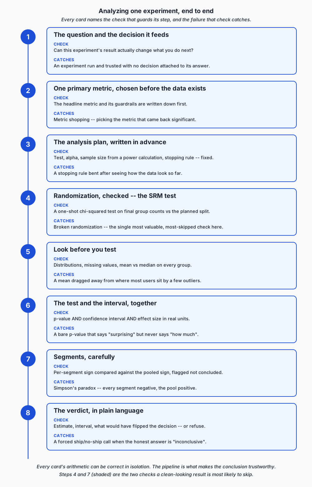
- Run the eight-step end-to-end analysis process in order -- question, pre-registered metric, written plan, randomization check, look-before-you-test, test-with-interval, careful segments, plain-language verdict -- and name the specific failure mode each step guards against
- Build a sample-ratio mismatch check from a chi-squared goodness-of-fit test with a closed-form p-value (math.erfc), run it once over final counts rather than continuously, and explain why it is the single most valuable and most-often-skipped check in this process
- Report a primary metric's result as a confidence interval AND an effect size in its own units (absolute and relative), never as a bare p-value, using the same math.erf-based normal CDF Day 118 built
- Detect and correctly flag a Simpson's-paradox-shaped segment reversal -- every segment pointing one way, the pooled number pointing the other -- on a real measured dataset, and explain why segment analysis must report findings rather than conclude from them
- Demonstrate, on one real dataset walked in arrival order, why a running p-value crossing below 0.05 partway through data collection is not the same evidence as the same p-value observed at a pre-declared sample size
- Build a verdict function that ships a clean experiment and explicitly REFUSES to compute an effect estimate at all once randomization has failed its own check, and explain why that refusal is itself the correct output
- Distinguish statistical significance from practical significance as a decision problem (cost of shipping and maintaining versus size of the affected population), and treat "inconclusive" as a legitimate first-class outcome rather than a failure
- Explain the checkout-experiment discipline's direct analogue in AI practice: a pre-registered offline evaluation metric, a guardrail that can veto a winning model, a held-out set sized by a power calculation, and a reported interval rather than a single leaderboard number
Prerequisites
- Day 116 -- descriptive statistics, the mean-versus-median divergence under outliers, and Simpson's paradox as a phenomenon; this lesson measures both on real simulated data
- Day 117 -- the standard error and its 1/sqrt(n) law, used implicitly in every confidence interval this lesson computes
- Day 118 -- hypothesis tests, confidence intervals, the normal CDF built from math.erf, multiple comparisons, power, and the cost of peeking. This lesson assumes that machinery and applies it to one experiment end to end rather than re-deriving it
- Comfort with the standard library csv, statistics and math modules
- Days 71-74 -- running pytest and reading its skip-versus-fail output
Why this matters
Here is an experiment that looks entirely respectable. Forty thousand users, twenty thousand per arm. A conversion rate that moved from 10.1% to 11.9% — an 1.8 percentage point lift. A p-value of 0.03. A 95% confidence interval on the difference that excludes zero. Every rule Day 118 taught you says: ship it.
Now here is one more fact about that same experiment. The analyst who ran it looked at seven different metrics before landing on “conversion rate” as the headline, and this is the one that came back significant. Or: the realized split was 52% treatment, 48% control, against a planned 50/50 — nobody checked. Either fact, on its own, is enough to make the entire result evaporate. Not weaken it. Not add a caveat to it. Evaporate it — turn it from evidence into noise that happened to look like evidence.
Notice what did not happen in that second paragraph: nothing about the arithmetic was wrong. The p-value was computed correctly. The confidence interval was computed correctly. If you re-ran Day 118’s formulas on the same numbers, you would get the same 0.03. The problem is not in the calculation. The problem is in everything the calculation cannot see — how the metric got chosen, whether the two groups were actually comparable, whether the number in the report is the number that was decided on in advance or the number that happened to survive.
This is the sentence to hold onto for the rest of this lesson: statistical validity is a property of the process that produced the number, not of the number itself. A p-value cannot certify the process that generated it. It can only certify that, given the process worked as assumed, this particular outcome would be unlikely under the null. If that assumption is false — if the metric was chosen after peeking, if the randomization silently broke, if the “significant” segment was found by trying twelve segments — the p-value is still a real number, correctly computed, and it is still evidence of nothing.
Day 118 built the machinery: hypothesis tests, confidence intervals, permutation tests, power, the cost of testing many things at once, the cost of peeking. This lesson does not re-derive any of that. It assumes you have it, hands you one complete experiment — actually two, generated by the same seeded script and shipped as CSV files you will load and analyze directly — and walks the process end to end: the question, the metric chosen in advance, the plan written down before the data existed, the check on whether the randomization itself can be trusted, a careful look at the data before testing it, the test and the interval together, the effect size in real units, a guardrail that can veto a good-looking result, a segment breakdown that generates hypotheses rather than confirming them, and a verdict in plain language. One of the two experiments you will analyze is exactly as clean as it looks. The other looks just as clean and is not — and by the end of this lesson you will have built the two checks that catch it, on real numbers, not a hypothetical.
The idea in plain language
Imagine handing two different people the exact same spreadsheet of raw experiment data and asking each of them, independently, to tell you whether the change should ship. If they can follow different, undocumented paths to get there — pick whichever metric looks best, stop collecting data whenever the number looks good, slice by whatever segment tells the story they want — they can each arrive at a different, defensible-looking answer from the same data. That is not a hypothetical failure mode. It is the default outcome of analyzing an experiment without a process, because there are dozens of small, individually reasonable-looking decisions along the way, and each one nudges the final number.
The fix is not more statistics. The fix is a process with no wiggle room in it: decide the metric before you see the data, decide the sample size and the stopping rule before you see the data, check that the randomization actually worked before you trust anything computed from it, and treat segment findings as things to investigate later, never as things that changed your mind today. Everything downstream of those decisions can use exactly the machinery Day 118 built. The discipline is entirely in what happens before you touch the primary test.
Historical background
The idea that an experiment’s design — not just its analysis — determines whether its conclusions can be trusted goes back to Ronald Fisher’s agricultural field trials in the 1920s. Fisher insisted on randomization, replication, and a plan fixed before the harvest, precisely because farmers (and scientists) are extremely good at finding a story in data after the fact, and a plan written in advance is the only defense against telling yourself that story. His 1935 book The Design of Experiments is where “pre-registration,” in spirit if not in name, starts.
Online A/B testing inherited this discipline and then, for about a decade, largely lost it. The tools got so cheap to run — spin up a test, watch a live dashboard, ship the moment the green checkmark appears — that the old discipline of writing the plan down first quietly disappeared from a lot of practice, even as the statistical machinery got more sophisticated. Two things brought it back. First, a wave of industry papers from companies running thousands of experiments a year (Microsoft’s Experimentation Platform team, Google, Netflix, Airbnb) that documented, in public, how often naive “peek and stop” analysis produced results that did not replicate. Second, the sample-ratio mismatch check itself — popularized largely through a 2019 paper by Fabijan, Dmitriev, Olsson and Bosch, “Diagnosing Sample Ratio Mismatch in Online Controlled Experiments” — which gave practitioners a single, cheap, mechanical test that catches an entire category of silent randomization failures that no amount of statistical sophistication downstream can fix.
Simpson’s paradox, the segment-reversal failure this lesson’s second dataset is built around, is older still — first noted by Karl Pearson’s group around 1899 and formally described by Edward Simpson in 1951, though it was UDNY Yule who had described the same phenomenon decades earlier. It shows up here not as a historical curiosity but as a live risk in exactly the kind of segment breakdown every experimentation dashboard invites you to run.
What it is — and what it is not
Analyzing an experiment end to end is the discipline of running a fixed sequence of checks, in a fixed order, each guarding against one specific way a technically-correct calculation can support a false conclusion. It is not a new statistical test — every test used in this lesson’s lab is one Day 118 already built. It is not a substitute for the machinery of hypothesis testing; it is the scaffolding that makes that machinery trustworthy.
It is also, specifically, not “running more tests to be extra careful.” A team that runs the primary test, then also tests ten segments, then also tests three secondary metrics, each at the same significance threshold, has made the multiple-comparisons problem worse, not better — Day 118’s lesson, wearing a different hat. End-to-end analysis is disciplined in the other direction: fewer decisions made after seeing the data, not more tests run against it.
Finally, it is not a guarantee. A properly analyzed experiment, with every check passing, can still be wrong — a 95% confidence interval is wrong about 5% of the time by design, and “inconclusive” is sometimes the correct, final answer. What end-to-end analysis buys you is not certainty; it is that your error rate matches the number on the label, instead of being silently far worse because of a process failure the arithmetic could never have revealed.
Why it was created and what problems it solves
Three concrete failure modes motivate every step in this lesson, and all three produce a result that is statistically significant and wrong, which is a more dangerous failure than an honest “we don’t know.”
Metric shopping. Test enough metrics against the same data and, by chance alone, roughly one in twenty will cross p < 0.05 even if nothing real is happening — Day 118’s multiple-comparisons arithmetic, applied to metric choice instead of segment choice. The fix is deciding the primary metric before the data exists, in writing, so there is nothing left to shop among.
Randomization that silently breaks. A caching layer that serves stale bucket assignments to one arm more than the other. A bot filter that disproportionately excludes one group. A retry-on-timeout path that reassigns slow-connection users. None of these announce themselves. All of them make the two groups no longer comparable, which invalidates every downstream comparison regardless of how careful the test itself is. The sample-ratio mismatch check exists because this failure mode is common, silent, and mechanically detectable — and, per the brief for this lesson, it is the single most valuable check here and the one most often skipped.
Peeking. Checking significance every day and stopping the moment p < 0.05 turns a nominal 5% false-positive rate into something dramatically higher, because you are effectively running the test many times and taking the best of them. Day 118 demonstrated this in simulation. This lesson demonstrates it on one real dataset: exercise 8 walks a genuinely significant experiment in arrival order and watches its running p-value dip below 0.05 partway through, climb back above it, and only settle for good much later — which is exactly the instability a fixed, pre-declared stopping rule protects you from, even when, as here, the final answer turns out to be correct anyway.
How it works
The process is eight steps, run in this order, each one guarding against a specific failure the previous steps cannot catch.
1. The question and the decision it feeds. Before anything statistical happens, state the decision this experiment will change. “Does the new checkout button increase conversion enough that we should ship it to everyone?” is a question with a decision attached. “Is the new button better?” is not — “better” by what measure, by how much, compared to what cost? An experiment that cannot change what you do next is not worth running, whatever its p-value says. Its failure mode is not statistical at all: it is running (and trusting) analysis on a question nobody could have acted on differently either way.
2. One primary metric, chosen before the data exists, plus guardrails that must not worsen. Exactly one number is the headline. Everything else is either a guardrail (must not get worse, by a pre-declared tolerance) or purely exploratory. Choosing the primary metric after looking at the data converts Day 118’s multiple-comparisons problem into a hidden, undocumented version of the same problem — the analyst does not even need to run seven tests explicitly; skimming seven metrics and mentally settling on the one that “looks interesting” has the identical statistical effect.
3. The analysis plan, written in advance. The test to be used, the significance level (α), the sample size computed from a power calculation, and the stopping rule — fixed horizon, or a named sequential procedure if you are deliberately using one. This is the direct defense against step 6’s peeking failure: a rule you commit to before the data exists cannot be bent by what the data later show.
4. Randomization, checked, not assumed. This is the sample-ratio mismatch (SRM) check, and it deserves its own weight in this list. If you planned a 50/50 split and the realized counts came out 52/48 at a large sample size, that is not a rounding error — it is itself a testable hypothesis, using the exact chi-squared machinery from a goodness-of-fit test, and at large n even a small realized skew clears significance easily. Failing this check invalidates everything computed afterward, because the two groups are no longer guaranteed comparable — whatever silently biased the assignment may have biased the outcome too. This is the check the brief for this lesson calls the single most practically valuable one here, and the one most often skipped, because it is boring, mechanical, and easy to forget when the primary metric already looks good.
5. Look before you test. Distributions, missing values, and the outliers Day 116 showed a mean cannot survive. A metric with a handful of extreme values (bot traffic, a logging glitch, a single whale customer) can have its mean dragged somewhere the median never moves — checking both, on every group, before running any test, is cheap insurance against exactly that.
6. The test and the interval, together. The hypothesis test answers “would we be surprised by this outcome if there were truly no effect?” The confidence interval answers a different, more useful question: “what range of true effect sizes is consistent with what we observed?” Report both. A p-value with no interval tells a reader whether to be surprised; it tells them nothing about how big the effect might actually be, nor how uncertain that size is.
7. Segments, carefully. Day 116’s Simpson’s paradox is not a curiosity here — it is a live risk in the single most common thing a stakeholder asks for after seeing a positive result: “break it down by region,” “break it down by device,” “break it down by user tenure.” An effect can be positive in every segment and negative overall, or vice versa, when the segment mix differs between the two arms. Segment fishing — testing every segment at the full significance threshold and reporting whichever one is “interesting” — is Day 118’s multiple-comparisons trap wearing a friendly, business-stakeholder-approved face. The honest rule, stated plainly: segments generate hypotheses, they do not confirm them.
8. The verdict, in plain language. State the estimate, its interval, and — this is the part almost always skipped — what value the interval would have needed to exclude for the decision to flip. “Inconclusive” is a legitimate, first-class outcome here, not a failure of the experiment and not something to round silently into “no effect.”
Three things are worth naming explicitly before you touch the lab. Novelty effects: a genuinely new UI element can move a metric purely because it is new and users are curious, an effect that fades over days or weeks — a treatment that looks strong on day one and fades by day fourteen is not necessarily “the effect wearing off,” it may be the effect never having existed beyond curiosity, and the fix is either running longer or explicitly measuring only returning users. Statistical versus practical significance: an interval that excludes zero but sits entirely between 0.01% and 0.03% lift is statistically significant and may not be worth the engineering cost of shipping it — significance is a question about noise; whether an effect is worth acting on is a decision problem that also needs the cost of shipping, the cost of maintaining, and the size of the population affected. Inconclusive is not failure: when the confidence interval spans both a value you would ship and a value you would not, the honest answer is “we don’t know yet,” not a coin flip dressed up as a conclusion.
An everyday analogy
A single technically-correct measurement is like one accurate reading from a thermometer that was left, unnoticed, next to an open window. The reading itself — 61°F — was measured correctly; the thermometer’s calibration was fine; the arithmetic that converted the sensor’s voltage into a number on the display did not make a single mistake. And it still tells you nothing true about the room, because the process that produced the measurement — where the thermometer happened to be sitting — was broken in a way no amount of care in reading the display could fix.
End-to-end experiment analysis is checking where the thermometer was sitting before you trust what it says. The sample-ratio mismatch check is opening your eyes and looking at the window. The segment analysis is walking around the room with a second thermometer to see if the story holds up in every corner before you repaint based on one number. None of this replaces reading the thermometer correctly — Day 118 already taught you that. It is the part that decides whether the number you read correctly was ever worth reading in the first place.
Examples in practice
Every worked number in this section, and in the lab, comes from the two datasets shipped with this lesson’s lab: exp_a.csv (16,000 rows, a clean checkout experiment) and exp_b.csv (20,000 rows, the same nominal experiment, haunted). Both are simulated and generated deterministically by a seeded script — never real user data — and every figure below is a genuine measurement from running the reference pipeline against those files, captured on this lesson’s authoring machine.
Dataset A, step by step. The plan: primary metric is conversion rate, planned split 50/50, guardrail is page-render latency (must not worsen by more than 5ms). Step 4, the SRM check: 8,000 control, 8,000 treatment, exactly the planned split, chi-squared p-value 1.0 — passes cleanly. Step 5, the look: time-on-page has a mean of 74.16 seconds against a median of 49.55 seconds in the control group (72.12 vs 49.28 in treatment) — a real, planted handful of bot-like sessions in the thousands-of-seconds range dragging the mean well away from where a typical visitor actually sits, Day 116’s lesson confirmed on data nobody flagged as containing outliers. Step 6, the test: conversion moved from 10.13% to 11.91%, a difference of 1.79 percentage points, z = 3.61, p = 0.0003, 95% confidence interval [0.82, 2.76] percentage points — excludes zero comfortably. Step 7, the effect size: a 17.65% relative lift, reported alongside the absolute 1.79 points, never alone. Step 8, the guardrail: control latency 219.77ms, treatment 219.26ms — treatment is, if anything, marginally faster, comfortably inside the 5ms tolerance. Step 9, segments: desktop +2.50pp, mobile +1.78pp, tablet −0.08pp — two segments agree with the pooled direction, tablet sits close enough to zero that it is noise, not a reversal, and the segment analysis correctly declines to flag anything. Verdict: ship.
Dataset B, step by step — same pipeline, opposite ending. Same nominal experiment, same plan, same primary metric. Step 4, the SRM check: 9,600 control, 10,400 treatment — a realized split of 48%/52% against the planned 50/50, chi-squared p-value 1.5 × 10⁻⁸, decisively below even a conservative α = 0.001 threshold. The check fails. At this point the correct action is to stop — not to compute the primary test and report it with an asterisk, but to refuse to compute a trustworthy estimate at all, because the two groups are no longer known to be comparable. If you continue anyway (as this lesson’s lab does, deliberately, so you can see what the broken numbers would have said), the primary metric shows conversion moving from 7.46% to 11.35%, a 3.89 percentage point lift, p effectively zero to double precision, a confidence interval of [3.08, 4.69] points — a far more impressive-looking result than dataset A’s. And the segment breakdown shows exactly why it cannot be trusted: every one of the three segments — desktop (−3.56pp), mobile (−2.48pp), tablet (−4.30pp) — shows a negative effect, while the pooled number shows a positive one. This is a genuine, measured Simpson’s paradox: the treatment arm was stuffed with a disproportionate share of the desktop segment (which converts at a much higher base rate than mobile), so pooling makes a uniformly negative effect look like a strong positive one. Verdict: do not trust this result — and the verdict function refuses to hand back an effect estimate at all, because step 4 already failed.
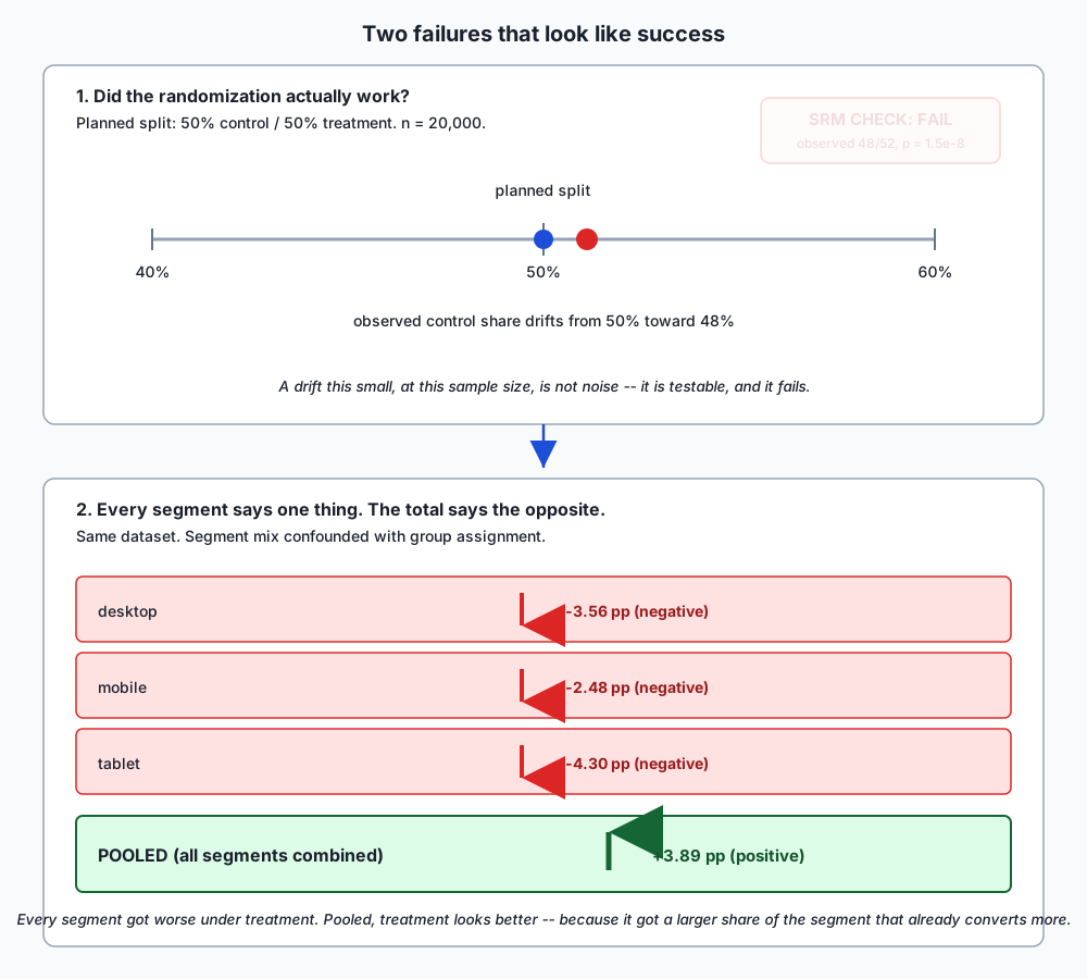
The two datasets are the same size class, use the same columns, and would look equally clean in a one-line summary (“conversion up, guardrail fine”). The only thing that tells them apart is running the checks that most dashboards skip.
Implications: security, privacy, performance, scalability, and cost
Security. A sample-ratio mismatch is very often a symptom of a real engineering bug with security-shaped roots: a caching layer serving one arm’s assignment more than the other’s, a bot-filtering rule that silently excludes a disproportionate share of one group, a retry path that reassigns users on slow or flaky connections. The SRM check does not diagnose the cause. It is the smoke alarm that tells you to go find one before you act on anything downstream.
Privacy. Segment analysis is exactly where privacy risk concentrates, because “break it down by X” tends toward finer and finer slices, and a sufficiently fine slice can re-identify individuals even without any name attached. Any segment small enough that its counts could single someone out (a segment of three users in one region on one device model) should be aggregated up or suppressed before it is ever reported, independent of whether its effect looks interesting.
Performance and scalability. Every calculation in this lesson’s lab — the SRM chi-squared test, the two-proportion z-test, the confidence interval, the per-segment breakdown, walking a dataset in arrival order for the peeking demonstration — is a single pass or two over the data, entirely closed-form. None of it requires simulation at analysis time (the bootstrap from Day 117 does, but it is not needed here because the primary metric is a proportion with a well-behaved closed-form standard error). At the scale of a real experimentation platform processing millions of rows per experiment, this matters: a closed-form test that runs once over aggregated counts scales trivially, while a naive per-row streaming significance check — recomputed on every new event to feed a live dashboard — is exactly the peeking pattern that inflates the false-positive rate, independent of how cheap it is to compute.
Cost. The real cost of skipping end-to-end discipline is not the analysis time saved by skipping it — it is the cost of shipping a change that does not actually work, discovered only after the fact, or worse, never discovered at all because the SRM-broken result looked clean enough that nobody re-checked it. A five-minute chi-squared test is cheap. A shipped feature built on a Simpson’s-paradox-inverted conclusion is not.
Alternatives: free, open source, and commercial
The tools that implement pieces of this pipeline range from “write it in twenty lines with the standard library” to full commercial experimentation platforms. Two were actually run for this lesson’s lab; two were not and are described from their documentation, honestly marked as such.
| Tool | When to choose it | How it’s used here | Free vs paid |
|---|---|---|---|
Hand-rolled with math.erf/erfc and csv | You want to understand exactly what the test computes, or you are in an environment (like this lab’s) with no scientific-computing stack available | Every test in this lesson’s lab — the SRM chi-squared test, the two-proportion z-test, the confidence interval — is built this way, and every number in the Examples section above came from running it | Free, standard library only |
Python’s statistics module | Quick descriptive summaries (mean, median, stdev) without pulling in a dependency | group_summary in this lesson’s lab uses statistics.mean, statistics.median and statistics.stdev directly | Free, standard library |
scipy.stats | Production analysis code where correctness-critical routines (Welch’s t-test, chi2_contingency, exact binomial tests) should come from a heavily reviewed, widely used library rather than a bespoke implementation | Not installed in this lesson’s environment; described from its documentation, not run. scipy.stats.ttest_ind would replace this lesson’s hand-rolled two-sample test, and scipy.stats.chi2_contingency would replace the hand-rolled SRM check | Free, open source (BSD) |
statsmodels | Sequential testing, power analysis, and proportion tests with more configuration than scipy.stats exposes directly (statsmodels.stats.proportion.proportions_ztest, power calculators) | Not installed in this lesson’s environment; described from its documentation, not run | Free, open source (BSD) |
| pandas | Segment breakdowns on real tabular data, once you have more than a handful of segment columns | Not installed in this lesson’s lab, by design. Its DataFrame.groupby("segment") would replace exercise 7’s hand-written loop over sorted segment names with one line; Week 18 teaches pandas properly, and this lesson does not assume it yet | Free, open source (BSD) |
| A commercial experimentation platform (Optimizely, LaunchDarkly’s experimentation module, Statsig, Eppo) | A team running many concurrent experiments that wants the plan, the SRM check, sequential testing and the dashboard integrated, with an audit trail of what was pre-registered | Not used in this lesson. These platforms implement the same eight-step process described in this lesson, packaged as a product, with the SRM check typically built in and surfaced automatically | Commercial, usage- or seat-based pricing, most with a limited free or trial tier |
The honest comparison: nothing in the paid tools does statistics the hand-rolled version cannot. What they buy is workflow — enforcing that the plan gets written down before the experiment starts, surfacing the SRM check automatically so it cannot be skipped, and an audit trail for what was pre-registered versus discovered after the fact. That workflow enforcement is real value; it is also exactly the discipline this lesson asks you to practice by hand first, so that a platform’s automation reads as a safety net rather than a black box.
Comparison with related concepts
| Concept | What it answers | How it relates to today |
|---|---|---|
| Hypothesis test (Day 118) | “Would this outcome be surprising if there were truly no effect?” | One step (step 6) inside the eight-step process this lesson teaches; today does not add a new test, it adds the process around the ones you already have |
| Confidence interval (Day 118) | “What range of true effect sizes is consistent with the data?” | Paired with the test at step 6; this lesson insists the two are always reported together, never the test alone |
| Sample-ratio mismatch check | ”Did the randomization itself work?” | New today. A precondition check, not an effect-size test — it must pass before step 6’s result can be trusted at all |
| Simpson’s paradox (Day 116) | “Can a pooled trend reverse when you look inside the groups that make it up?” | Today shows it live, in a segment breakdown, as a risk that a positive-looking A/B result can hide rather than as an abstract phenomenon |
| Multiple comparisons (Day 118) | “What happens to my false-positive rate when I test many things?” | Underlies both metric shopping (step 2) and segment fishing (step 7) — the same statistical mechanism, wearing two different practical disguises |
| Peeking / optional stopping (Day 118) | “What happens to my false-positive rate if I check repeatedly and stop early?” | Demonstrated today on one real, genuinely significant dataset rather than in simulation, to show the instability directly |
| A/B test power analysis (Day 118) | “How large a sample do I need to reliably detect an effect of a given size?” | Feeds step 3’s pre-registered sample size; not re-derived today, assumed as an input to the plan |
When to use it — and when not to
Use the full eight-step process whenever a decision with real cost — shipping a feature, changing a default, launching a pricing change — will be made from an experiment’s result. That is nearly every production A/B test, and it is exactly what this lesson’s lab walks through twice.
You can reasonably compress the process for genuinely low-stakes, easily reversible changes where the cost of a wrong call is small and the cost of running the full pipeline exceeds the cost of occasionally being wrong — an internal tool tweak seen by twelve engineers, say. Even there, the SRM check is cheap enough (a few lines, one pass over the data) that skipping it saves almost nothing.
Do not use significance testing at all — full pipeline or not — as a substitute for a decision you could make more directly. If an engineering change is a strict improvement with no plausible downside (a genuine bug fix, a real latency reduction with no behavior change), running an A/B test to “prove” it helped is often theater: ship it, monitor guardrails, and save the statistical machinery for changes whose effect is genuinely uncertain in either direction.
Knowledge check
- An experiment reports a clean 1.8 percentage point lift, p = 0.03, and a confidence interval excluding zero. What single additional fact, on its own, could make this result worthless as evidence?
- Why does the sample-ratio mismatch check need to be run once, over the final counts, rather than continuously as data streams in?
- In dataset B, every one of three segments shows a negative effect, but the pooled effect is positive. What has to be true about the segment mix for this to happen?
- Why does this lesson insist the effect size (in percentage points and relative lift) always accompany the p-value, rather than the p-value being reported alone?
- A guardrail metric passes on dataset A even though the primary metric shows a strong positive lift. What role does the guardrail play in the final verdict that the primary test alone cannot?
- Dataset A’s running p-value, checked every 500 rows, dips below 0.05 at row 4,000 and rises back above it by row 5,000. What does this demonstrate about a policy of stopping the instant p < 0.05 is first observed?
- Why is “the treatment beat the control by 3.89 percentage points, p effectively zero” from dataset B not good news, despite being a larger and more significant-looking effect than dataset A’s?
- What is the difference between reporting a segment’s finding as a “hypothesis” versus reporting it as a “conclusion,” in terms of what the analyst does next?
Hands-on exercise
Build the nine-function pipeline this lesson’s Examples section walked through, and run it against both shipped datasets yourself.
Work through starter/00_brief.md in the lab, implementing each of the nine functions in starter/experiment.py:
load_experiment(path)— parse the CSV, validate columns and group labels, reject missing values.srm_check(rows, planned_split, alpha)— the chi-squared goodness-of-fit test on final group counts, usingmath.erfc(math.sqrt(chi2 / 2))for the closed-form p-value.group_summary(rows, metric)— per-group mean, median, standard deviation, min, max.primary_test(rows, metric, conf)— the two-proportion z-test plus a confidence interval on the difference.effect_size(primary_result)— absolute difference in percentage points, plus relative lift.guardrail_check(rows, metric, tolerance, lower_is_better)— a metric that can veto an otherwise-positive result.segment_analysis(rows, metric)— per-segment lift alongside the pooled lift, with a reversal flag.peek_path(rows, metric, checkpoint_every)andcrossed_significance(path, alpha)— the running p-value walked in arrival order.verdict(srm_result, primary_result, guardrail_result, segment_result, alpha)— the final plain-language decision, including the refusal case.
Check your progress at any point with .venv/bin/pytest starter -q — unattempted functions report as skipped, wrong ones fail with your answer shown beside the correct one.
Expected output
Running .venv/bin/pytest examples -q against the reference implementation reports 12 passed. The nine numbered scripts in examples/ each print their step’s real numbers and end with a line reading <script>.py: every assertion held. — for example, 02_sample_ratio_mismatch.py prints dataset A’s SRM check passing with p_value=1.000000 and dataset B’s failing with p_value=1.542e-08, and 09_verdict.py prints verdict: ship for dataset A and verdict: do not trust this result with refused: True for dataset B. The full harness, bash tests/run_tests.sh, ends with the literal line 35 checks, 0 failure(s). and exits 0.
Validate your work
cd labs/sections/math-statistics-and-data/day-119-analyzing-an-experiment-end-to-end
python3 -m venv .venv
.venv/bin/pip install -r requirements/requirements.txt
.venv/bin/pytest starter -q
bash tests/run_tests.sh; echo "exit=$?"
A correct, complete starter/experiment.py reports 11 passed from pytest starter -q. The full harness should report exit=0.
Troubleshooting
If srm_check passes on dataset B (it should fail), check that expected_control and expected_treatment are computed from n * planned_split, not from the observed counts themselves — computing “expected” from what was actually observed makes the chi-squared statistic zero by construction on every dataset, every time. If segment_analysis never flags dataset B’s reversal, check that the flag requires every segment’s sign to disagree with the pooled sign, not just one — a single near-zero segment (like dataset A’s tablet segment) should not trip it. The lab’s troubleshooting.md covers these and several other issues actually hit while building this lab, including the peeking walk’s row-order dependency and a note on why dataset B’s p-value prints as 0.0 (floating-point underflow on a genuinely tiny value, not a bug).
Common mistakes
Reporting primary_test’s p-value without also computing effect_size — a p-value alone cannot distinguish “significant and tiny” from “significant and large.” Running segment_analysis and reporting the segment with the most extreme p-value as if it were confirmed, rather than flagged as exploratory. Skipping the SRM check because the primary metric already “looks fine” — dataset B’s primary metric looks better than dataset A’s, which is exactly why the check has to run regardless of how the headline number looks. Computing the guardrail check but not wiring its result into the final verdict, so a guardrail failure gets silently reported in a side table instead of vetoing the “ship” decision.
Practice assignment
Using the two shipped datasets and your completed experiment.py, write a two-paragraph memo addressed to a product manager who has only seen dataset B’s headline number (a 3.89 percentage point lift, “highly significant”). The first paragraph should explain, in plain language with no jargon, why this result cannot be trusted — naming both the sample-ratio mismatch and the segment reversal, and stating what you would need to see instead before recommending a decision. The second paragraph should state, honestly, what you would tell them to do next: re-run the experiment with the randomization bug fixed, or investigate the caching/assignment issue first, or something else — and why.
Extension challenge
Modify examples/generate_data.py to produce a third dataset, exp_c.csv, where the sample-ratio mismatch check passes and the segment analysis shows no reversal, but the guardrail check fails badly enough that verdict() should report "do not trust this result" for a reason distinct from either of dataset B’s problems. Confirm your modified pipeline correctly distinguishes all three failure reasons (SRM failure, segment reversal as a caveat on an otherwise-shippable result, and guardrail failure) rather than collapsing them into one generic “something is wrong” message. Then write one paragraph on which of the three failure modes you judge hardest for a busy analyst to notice without an automated check, and why.
The tools built from scratch, and what building them buys you
Everything computed in this lesson’s Examples section — the SRM chi-squared test, the two-proportion z-test, the confidence interval, the segment breakdown — was built from math.erf/math.erfc and the standard library, deliberately, in an environment where scipy and statsmodels are not installed. This section says plainly what that means: no output attributed to either package anywhere in this lesson or its lab was actually produced by them, and both are described from their public documentation rather than run.
That constraint turned out to be pedagogically useful rather than merely limiting. scipy.stats.chi2_contingency would replace the SRM check’s dozen lines of arithmetic with one function call — and having written the dozen lines first, the function call’s inputs and outputs stop being opaque. The same is true of scipy.stats.ttest_ind against this lesson’s hand-rolled two-proportion z-test, and of statsmodels.stats.proportion.proportions_ztest against the same. pandas.DataFrame.groupby("segment") would replace exercise 7’s explicit loop over sorted segment names with a single line — Week 18 teaches pandas properly, and this lesson deliberately does not lean on it before then, but the shape of what groupby is doing (partition the rows by segment value, apply the same test to each partition, collect the results) is now something you have implemented by hand once, on real data, before you ever call it.
The AI thread
Shipping a new model version is an A/B test, whether or not anyone on the team calls it one, and every failure mode in this lesson has a direct AI-practice analogue. The primary metric — task success rate, win rate against a reference model, a specific downstream business metric — has to be pre-registered before the evaluation runs, or “we tried a few metrics and this one looked best” quietly becomes the same metric-shopping problem this lesson opened with. A guardrail — latency, cost per request, refusal rate on a held-out safety set — has to be able to veto a model that wins on the headline metric but got there by getting slower, more expensive, or less safe; a positive eval score with no guardrail attached is exactly as trustworthy as dataset A’s checkout lift would have been without the latency check. The held-out evaluation set has to be large enough for the effect size you actually care about — the same power calculation from Day 118, run before the evaluation, not after someone asks “was that gap real?” And the result has to be reported as an interval, never a bare number: “the new model scored 91.4% versus 91.1%” is the same 0.3-point gap Day 117’s binomial standard error calculation showed sitting comfortably inside noise on a 500-example test set. The discipline this lesson teaches on a checkout button generalizes completely: whether the thing being compared is a UI change or a model checkpoint, the question “was this evidence, or did the process that produced it just look like evidence” is answered exactly the same way.
Quiz
Q1. An experiment reports a clean 1.8 percentage point lift, p = 0.03, and a 95% confidence interval excluding zero. The analyst mentions, almost in passing, that they looked at seven different metrics before landing on this one. What does this fact do to the result?
- It only matters if the seven metrics were all correlated with each other
- It would matter if the metrics had been tested with a t-test, but not with a z-test
- Nothing -- the p-value was computed correctly on the metric that was reported, so it remains valid evidence
- It converts a hidden multiple-comparisons problem into the result: testing seven metrics means roughly one in twenty would cross p<0.05 by chance alone even with no real effect, so the "significant" one may simply be the lucky one
Show answer
Answer: D. It converts a hidden multiple-comparisons problem into the result: testing seven metrics means roughly one in twenty would cross p<0.05 by chance alone even with no real effect, so the "significant" one may simply be the lucky one
Choosing the primary metric after seeing the data has exactly the same statistical effect as Day 118's multiple-comparisons problem, even though no formal correction was applied and the analyst may not have run seven explicit hypothesis tests -- skimming seven metrics and settling on the interesting one does the same damage. The fix is deciding the primary metric before the data exists, in writing, so there is nothing left to shop among.
Q2. Why must the sample-ratio mismatch (SRM) check be computed once, over the FINAL group counts, rather than continuously as data streams in?
- Because chi-squared tests are only valid on data collected within a single calendar day
- Because the chi-squared formula only accepts inputs collected in one batch
- It does not matter; checking continuously gives an equivalent result to checking once at the end
- Because a clean, genuinely 50/50 split will drift above and below 50/50 many times along the way by chance alone as data accumulates, so checking it repeatedly and flagging any mid-stream drift would itself be a form of peeking that trips on nearly every experiment
Show answer
Answer: D. Because a clean, genuinely 50/50 split will drift above and below 50/50 many times along the way by chance alone as data accumulates, so checking it repeatedly and flagging any mid-stream drift would itself be a form of peeking that trips on nearly every experiment
This is the SRM check's own version of Day 118's peeking problem: computing it at every intermediate row count would fire false alarms constantly, because a genuinely balanced random process still fluctuates around 50/50 along the way. Computing it once, over the final assigned counts, is what makes the test's stated alpha meaningful.
Q3. In dataset B, all three segments (desktop, mobile, tablet) show a NEGATIVE effect, but the pooled effect across all segments is positive. What must be true about the segment mix for this Simpson's-paradox-shaped reversal to occur?
- The segments must have identical base conversion rates
- The treatment and control groups must contain very different proportions of the segments, correlated with each segment's base rate -- for example, treatment stuffed with a high-base-rate segment and control stuffed with a low-base-rate one
- The sample size must be too small for the segment-level tests to have any power
- At least one segment must have exactly zero conversions
Show answer
Answer: B. The treatment and control groups must contain very different proportions of the segments, correlated with each segment's base rate -- for example, treatment stuffed with a high-base-rate segment and control stuffed with a low-base-rate one
In dataset B, the treatment arm received a much larger share of the high-converting "desktop" segment while control received a much larger share of the low-converting "mobile" segment. Even though EVERY segment truly performed worse under treatment, pooling mixes in more of the naturally-higher-converting segment on the treatment side, which flips the pooled sign. This is exactly why segment mix must be checked, not just segment-level significance.
Q4. Why does this lesson insist that an effect size (in the metric's own units, plus a relative lift) always accompany a reported p-value?
- Because a p-value cannot be computed without first computing an effect size
- Because regulators require both figures to be reported together
- Because a p-value alone answers "would this be surprising under no effect", but says nothing about how large the effect actually is or whether that size is worth acting on -- a tiny, practically meaningless effect can still be statistically significant
- Because relative lift and absolute difference are mathematically identical and reporting both is redundant but harmless
Show answer
Answer: C. Because a p-value alone answers "would this be surprising under no effect", but says nothing about how large the effect actually is or whether that size is worth acting on -- a tiny, practically meaningless effect can still be statistically significant
Dataset A's 1.79 percentage point absolute lift and 17.65% relative lift describe a result a reader can act on; "p=0.0003" alone does not. An interval that excludes zero but sits entirely between, say, 0.01% and 0.03% lift would also be statistically significant and might not be worth the engineering cost of shipping -- significance and "worth acting on" are different questions, and only the effect size lets a reader ask the second one.
Q5. Dataset A's guardrail metric (page-render latency) is checked alongside a primary metric that shows a strong, significant positive lift. What role does the guardrail play that the primary test alone cannot?
- It can VETO an otherwise-positive verdict if a metric that must not get worse (like latency) worsens beyond a pre-declared tolerance, regardless of how good the primary result looks
- It recomputes the same significance test on a different random seed, as a sanity check
- It replaces the primary test entirely once both are computed
- It only matters for continuous metrics, not binary ones like conversion
Show answer
Answer: A. It can VETO an otherwise-positive verdict if a metric that must not get worse (like latency) worsens beyond a pre-declared tolerance, regardless of how good the primary result looks
A primary metric moving in the right direction is not sufficient to ship -- a guardrail failure (latency getting meaningfully worse, an error rate rising, an unsubscribe rate climbing) must be able to change the final verdict from "ship" to something else, independent of how strong the primary result is. Dataset A's guardrail passed (latency actually improved slightly); the lesson's verdict function is built so a guardrail failure would have overridden a positive primary result.
Q6. Walking dataset A in its arrival order, the running p-value dips below 0.05 at row 4,000, climbs back above 0.05 by row 5,000, and only settles for good after row 5,500 -- even though the final, full-sample verdict at row 16,000 is also significant. What does this demonstrate?
- A team with a fixed, pre-declared stopping rule reaches the same well-supported conclusion at the planned sample size; a team that stops the instant it first sees p<0.05 would have stopped on an unstable fluctuation and gotten lucky that the sign did not flip -- exactly the risk a declared-in-advance stopping rule protects against, even when the eventual answer is correct
- The final verdict must be wrong, since an earlier reading disagreed with it
- The dataset was generated incorrectly and should be regenerated with a different seed
- The primary test formula must contain an error, since a genuinely significant effect should never show a p-value above 0.05 at any checkpoint
Show answer
Answer: A. A team with a fixed, pre-declared stopping rule reaches the same well-supported conclusion at the planned sample size; a team that stops the instant it first sees p<0.05 would have stopped on an unstable fluctuation and gotten lucky that the sign did not flip -- exactly the risk a declared-in-advance stopping rule protects against, even when the eventual answer is correct
This is a real, measured demonstration of Day 118's peeking-inflates-false-positives lesson, but on a dataset where the true effect IS real. The instability along the way is the point: a naive "stop the moment p<0.05" policy would have committed at row 4,000 on a reading that had not yet stabilized, and would have been indistinguishable, at the moment of stopping, from a false positive that later reverted.
Q7. Dataset B's primary metric shows a LARGER, MORE significant effect (3.89 percentage points, p effectively zero) than dataset A's (1.79 points, p=0.0003). Why is dataset B's result not better news?
- It is better news; a bigger, more significant effect is always stronger evidence regardless of any other check
- Because dataset B's sample-ratio mismatch check already failed (the realized split drifted to 48/52), which means the two groups are not known to be comparable, and the impressive-looking primary result is downstream of that same broken randomization -- the segment reversal is a second, independent symptom of the same underlying problem
- Because dataset B has more rows than dataset A, and larger sample sizes always produce less trustworthy p-values
- It is not worse news, only differently reported; both datasets should receive the same "ship" verdict
Show answer
Answer: B. Because dataset B's sample-ratio mismatch check already failed (the realized split drifted to 48/52), which means the two groups are not known to be comparable, and the impressive-looking primary result is downstream of that same broken randomization -- the segment reversal is a second, independent symptom of the same underlying problem
A bigger, cleaner-looking number computed downstream of broken randomization is not stronger evidence -- it is evidence of nothing, computed correctly. This is the lesson's central point: the arithmetic in dataset B is not wrong, the process that produced the data is, and no amount of statistical significance downstream of that can fix it. The verdict function refuses to hand back an effect estimate for exactly this reason.
Q8. What is the practical difference between reporting a segment finding as a "hypothesis" versus reporting it as a "conclusion"?
- There is no practical difference; both terms describe the same statistical result
- A "conclusion" requires a p-value below 0.01, while a "hypothesis" only requires a p-value below 0.05
- Reporting a segment finding as a hypothesis means treating it as something to investigate or test properly in a dedicated follow-up (with its own pre-registered plan and multiple-comparisons correction), while reporting it as a conclusion means acting on it directly -- which is exactly the segment-fishing failure mode this lesson warns against
- A hypothesis applies only to continuous metrics and a conclusion applies only to binary ones
Show answer
Answer: C. Reporting a segment finding as a hypothesis means treating it as something to investigate or test properly in a dedicated follow-up (with its own pre-registered plan and multiple-comparisons correction), while reporting it as a conclusion means acting on it directly -- which is exactly the segment-fishing failure mode this lesson warns against
Segments generate hypotheses, they do not confirm them -- testing every segment at the full significance threshold and acting on whichever one looks interesting is Day 118's multiple-comparisons problem wearing a business-stakeholder-friendly disguise. The honest path from a segment finding to a decision runs through a properly designed, pre-registered follow-up experiment, not straight into a ship/no-ship call.
Glossary
- Pre-registration
- Writing down the primary metric, the significance level, the sample size, and the stopping rule before the experiment's data exists, so none of them can be adjusted after the fact to make a result look better. The direct defense against metric shopping and segment fishing alike.
- Primary metric
- The single, pre-declared number an experiment is judged by. Every other metric is either a guardrail (must not worsen) or exploratory (reported, never concluded from). Choosing the primary metric after seeing the data converts a legitimate analysis into an undisclosed multiple-comparisons problem.
- Guardrail metric
- A metric that must not get worse by more than a pre-declared tolerance, and can veto an otherwise-positive verdict on the primary metric. In this lesson's lab, page-render latency is the guardrail -- dataset A's guardrail holds (latency improves slightly); a guardrail failure is designed to flip the final verdict regardless of how good the primary result looks.
- Sample-ratio mismatch (SRM)
- A statistically significant difference between the planned traffic split and the realized one -- for example, planning 50/50 and observing 48/52 at a large sample size. Detected with a one-shot chi-squared goodness-of-fit test over the final group counts. A failed SRM check means the two groups are not known to be comparable, which invalidates every downstream comparison regardless of how careful that comparison is.
- Chi-squared goodness-of-fit test
- A test comparing observed category counts against counts expected under a stated hypothesis (here, a 50/50 split). With two categories and one degree of freedom, the test statistic is the square of a standard normal variable, so its p-value has the closed form erfc(sqrt(chi2 / 2)) -- computable with nothing beyond the math module.
- Effect size
- How large an observed difference is, in the metric's own units (percentage points for a rate, seconds for a duration) and often also as a relative lift. Distinct from a p-value, which answers only whether the difference would be surprising under no true effect -- not how large it is or whether it is worth acting on.
- Simpson's paradox
- A pattern in which an effect points one way in every subgroup of a dataset and the opposite way when the subgroups are pooled, caused by the subgroups' relative sizes differing between the groups being compared. Measured directly in this lesson's dataset B, where every segment shows a negative effect while the pooled effect is positive.
- Segment fishing
- Testing many segments (region, device, tenure) at the same significance threshold used for the primary metric and reporting whichever one looks interesting, without correcting for the number of segments tested. The multiple-comparisons problem wearing a business-stakeholder-friendly disguise; the fix is treating segment findings as hypotheses for a dedicated follow-up, never as conclusions.
- Peeking (optional stopping)
- Checking an experiment's significance repeatedly during data collection and stopping the moment a threshold is crossed. Inflates the true false-positive rate well above the nominal alpha, because the analyst is effectively running many correlated tests and taking the most favorable one. Demonstrated in this lesson on real data: a genuinely significant experiment's running p-value dips below 0.05, rises back above it, and only stabilizes much later.
- Novelty effect
- A metric movement caused by a change being new and attracting curiosity, rather than by the change being genuinely better -- one that typically fades over days or weeks. A treatment that looks strong on day one and weaker by day fourteen may indicate the effect was never real beyond curiosity, not that "the effect wore off."
- Statistical versus practical significance
- Statistical significance answers whether an effect is distinguishable from noise; practical significance asks whether an effect, once distinguished from noise, is large enough to be worth the cost of shipping and maintaining it. A confidence interval that excludes zero but spans only a trivially small range can be statistically significant and not practically worth acting on.
- Inconclusive verdict
- A legitimate, first-class experiment outcome in which the confidence interval is too wide to rule out either "no meaningful effect" or "a meaningful effect" -- distinct from, and not silently rounded to, "no effect." The honest response is usually more data or a different design, not a forced ship/no-ship call.
- Verdict refusal
- The deliberate choice to return no effect estimate at all once a precondition check (here, the sample-ratio mismatch check) has failed, rather than computing and reporting a number anyway with a caveat attached. Used in this lesson's `verdict()` function: dataset B's verdict carries no `estimate_pp` key, because randomization that cannot be trusted makes any downstream number untrustworthy too.
Sources and further reading
- statistics — Mathematical statistics functions — Python Software Foundation (accessed 2026-08-19)
- math — Mathematical functions — Python Software Foundation (accessed 2026-08-19)
- csv — CSV File Reading and Writing — Python Software Foundation (accessed 2026-08-19)
- Random Generator — NumPy documentation — NumPy Developers (accessed 2026-08-19)
- scipy.stats.ttest_ind — SciPy documentation — SciPy Developers (accessed 2026-08-19)
- Statistics stats — statsmodels documentation — statsmodels Developers (accessed 2026-08-19)
Kept in this browser, no account needed. Your progress page turns the whole record into one link you can bookmark or open on another device.