Math, Statistics, and Data › pandas and Data Wrangling › Day 123

Day 123: Groupby and Aggregation

After this lesson you will be able to state and demonstrate that groupby drops rows with a missing key by default, silently, and show that the gap between a grouped sum and the overall sum equals exactly the missing-key rows' own total, then fix it with dropna=False; explain and demonstrate why size() and count() disagree exactly where a column has missing values; write .agg() four ways -- single function, list, per-column dict, and named aggregation -- and say which produces a flat column index and which produces a MultiIndex; state and demonstrate the shape difference between agg (one row per group) and transform (the input's shape), and use transform to build a within-group z-score; use GroupBy.filter to keep or drop whole groups by a predicate and explain how that differs from row-level filtering; build and read a multi-key groupby's MultiIndex, and produce the same values flat with as_index=False; explain what observed= controls for a categorical groupby and measure how many unobserved combinations the default manufactures; measure a built-in aggregation against the equivalent .apply(lambda ...) and report the gap as a ratio, never a millisecond figure; and compute a weighted mean per group with apply and again without it, checking that the two agree.

Learning objectives

By the end of this lesson you will be able to:

• Demonstrate that groupby(...).sum() silently excludes rows with a missing key by default, and that the gap between the grouped total and the overall total equals exactly the missing-key rows' own total
• Use dropna=False to make a groupby aggregation's parts sum back to the whole, and state this as a habit to run after every groupby aggregation
• Explain the difference between size() (rows) and count() (non-missing values per column) on a GroupBy object, and predict exactly where they will disagree
• Write .agg() four ways -- a single function, a list of functions, a per-column dict, and named aggregation -- and state which forms produce a MultiIndex on the result columns and which stay flat
• Demonstrate the shape difference between agg (one row per group) and transform (the input's shape), and use transform to attach a group mean back onto every original row
• Build a within-group z-score using transform for both the group mean and the group standard deviation, and verify each group's z-scores average to zero
• Use GroupBy.filter to keep or drop whole groups by a size or aggregate predicate, and explain how this differs from Day 122's row-level boolean-mask filtering despite sharing the word "filter"
• Build a multi-key groupby, read its resulting MultiIndex names and values, and produce the same result in a flat frame with as_index=False
• Explain what observed= controls for a categorical groupby, and measure how many unobserved category combinations the observed=False default manufactures on a two-key grouping
• Measure a built-in .agg() aggregation against the equivalent .apply(lambda ...) on the same data, and report the result as a ratio and a shape, never a millisecond figure
• Compute a weighted mean per group two ways -- with apply, and with a vectorised assign-then-agg route that avoids apply entirely -- and confirm the two results agree exactly
• State when SQL GROUP BY (executed where the data already lives) or pivot_table is the better choice over a plain pandas groupby, and describe polars' group_by as a documented design alternative

Prerequisites

• Day 120 -- pandas Series and DataFrames, index alignment, and Copy-on-Write; every table in this lesson is an ordinary DataFrame built the way that day taught
• Day 121 -- loading and inspecting data, the habit of checking a frame before trusting it
• Day 122 -- boolean masks, .query(), and the partition invariant (a filter that silently drops NaN rows so the halves no longer sum to the whole), which this lesson's exercise 1 directly extends to groupby
• Day 116 -- descriptive statistics and Simpson's paradox, which this lesson's AI-thread paragraph connects to per-group model evaluation
• Week 13 -- SQL and SQLite, the tool this lesson's Tools section compares groupby against for tabular questions already living in a database
• A working python3 on your PATH; the lab creates its own virtual environment with pandas 3.0.5 pinned exactly

Why this matters

Run this on pandas 3.0.5 and read the two numbers before anything else:

>>> orders.groupby("region")["amount"].sum().sum()
1945.0
>>> orders["amount"].sum()
2115.0

Same twelve rows. Same amount column. Two different totals, and pandas raised no exception, printed no warning, and returned a completely plausible-looking number both times. The gap — 170.0 — is not a rounding error and not a bug. It is exactly the amount on the two rows whose region was never recorded. groupby dropped them, silently, because dropna=True is the default, and nothing about the grouped output tells you it happened. The per-region report you just built looks complete. It is missing a category entirely: the rows nobody labelled.

That is the entire subject of this lesson, and it deserves to be said plainly rather than gently: groupby drops rows whose key is missing, by default, and the sum of your per-group totals will be less than the true total whenever that happens. A revenue report grouped by region that quietly omits every order whose region field was left blank is wrong in the direction nobody checks, because the number that comes out the other end is smaller, tidier, and entirely uncontradicted by anything pandas tells you. If your instinct is “that would show up as an obviously wrong number” — it does not. region_totals.sum() for this exact table returns 1945.0, a number with no red flag anywhere near it, and the person reading the dashboard has no way to know that 170 dollars of real revenue never made it into any bucket.

Day 122 taught this same shape of failure for boolean masks: a filter that drops NaN rows silently, so the kept half and the dropped half no longer sum back to the whole unless you specifically account for missing values. Today’s lesson is that exact invariant wearing a new costume. groupby is doing the same thing Day 122’s masks did — quietly deciding that a row with no label does not belong anywhere — except now it is happening inside an aggregation that produces numbers people put directly into reports, dashboards and models. The fix is one keyword, dropna=False, and the habit that catches this entire class of bug is one sentence, repeated at the end of nearly every exercise in this lesson: after any groupby aggregation, check that the parts reconcile with the whole.

groupby has a second, quieter trap sitting right next to the first one, and it is worth naming before you meet it in the wild: .size() and .count() sound like synonyms and are not. size() counts rows. count() counts non-missing values, per column. They agree everywhere the data is complete and disagree exactly where it is not — which means confusing them silently misstates a denominator in exactly the situation where getting the denominator right mattered most. Both are correct answers to two different questions, and pandas will happily let you ask the wrong one.

By the end of today you will be able to build a groupby aggregation four different ways, know precisely when to reach for agg versus transform versus apply, filter whole groups rather than individual rows, group by more than one key at once, control whether an unobserved categorical combination manufactures a phantom row, and measure — honestly, on this one machine, on this one day — how much a built-in aggregation beats the equivalent hand-rolled .apply. Every one of those skills sits on top of the same discipline the opening failure teaches: split, apply, combine, and always check that combine gave you back the whole.

The idea in plain language

Split, apply, combine. That is the entire mental model, and it is worth holding in exactly that order because pandas executes it in exactly that order, even when the code you write looks like one method call.

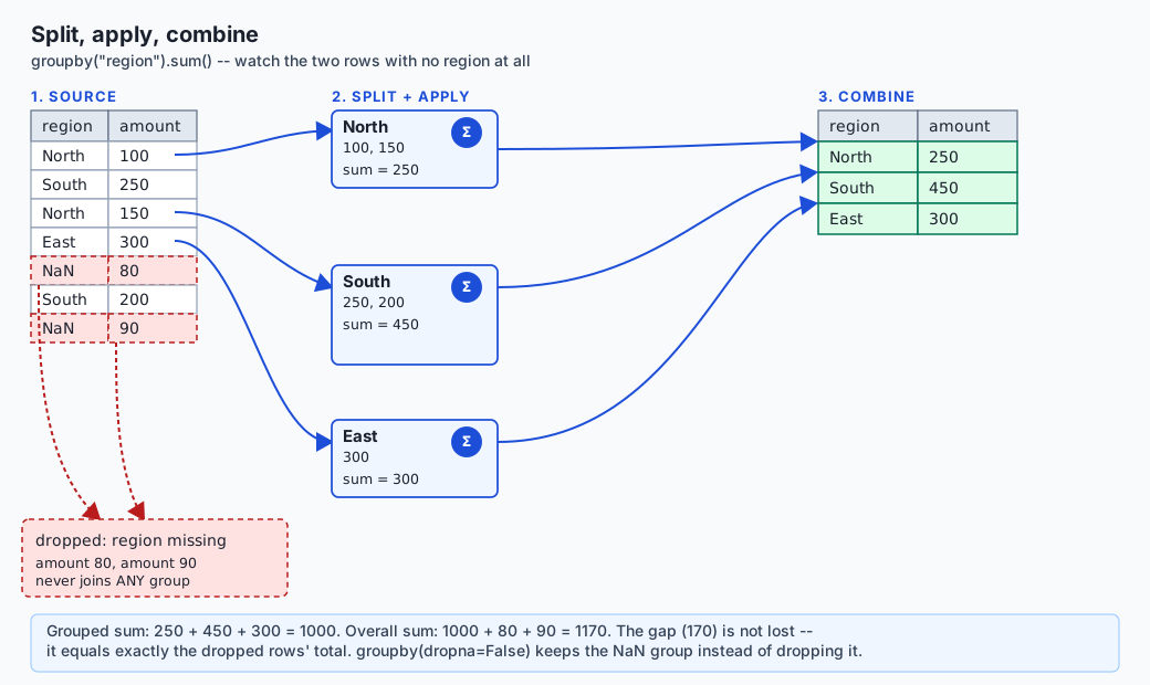
Split: pandas looks at the column (or columns) you grouped by and sorts every row into a bucket, one bucket per distinct value. A row with region = "North" goes in the North bucket. A row with region = "South" goes in the South bucket. A row whose region is missing — genuinely absent, NaN — goes, by default, nowhere. It is not placed in a bucket of its own; it is left out of the split entirely, which is the mechanism behind this lesson’s opening failure. If you want a bucket for the missing rows too, you have to ask for one explicitly with dropna=False.

Apply: whatever function you asked for — sum, mean, a NumPy function, a function you wrote yourself — runs once per bucket, on that bucket’s rows only. North’s function call never sees a South row. This is the part almost everyone already has right; it is the part most people underestimate.

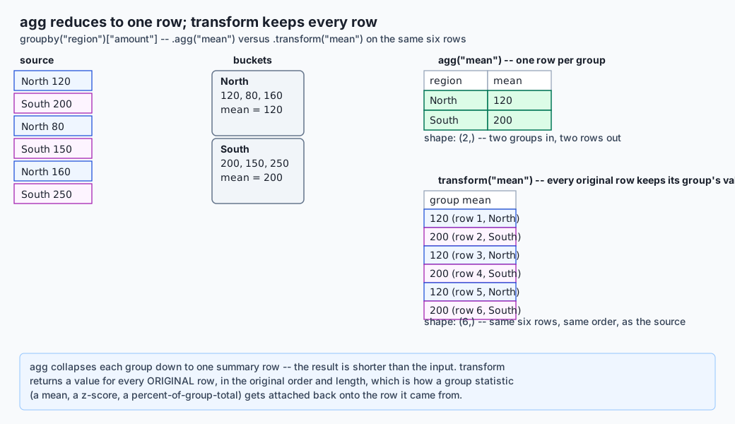
Combine: the per-bucket results get stitched back together into one final object. This is where the shape of your output is decided, and it is where the second half of this lesson’s subject lives: agg combines by shrinking each bucket down to one row, so a five-bucket grouping produces a five-row result no matter how many rows fed each bucket. transform combines differently — it hands every original row back its own bucket’s result, so the output has exactly as many rows as the input did, in the input’s own order. Same split, same apply, genuinely different combine, and the difference in shape is the whole reason both exist.

One more piece of plain language before the precise version: a GroupBy object does nothing on its own. Writing df.groupby("region") does not sum anything, does not sort anything into buckets yet in any way you can observe, and returns instantly no matter how large df is. It is a plan, not a result — pandas describes this as lazy. The actual split-apply-combine work happens only when you attach an aggregation: .sum(), .agg(...), .transform(...), or one of their relatives. Until then you are holding a DataFrameGroupBy object that has recorded your intention and computed nothing.

Picture the architecture diagram below. Six rows come in on the left. Two of them — the two whose region is blank — fall out at the split stage into their own tray, never reaching any group box, exactly as described above. The three groups that do form each get a function applied inside their own box, and the three per-group results combine into the final table on the right. The caption states the reconciliation explicitly: the grouped total plus the dropped rows’ total equals the true overall total, every time, by construction — which is exactly the arithmetic check you should be running on your own aggregations.

Now the shape distinction, animated. Six source rows — three North, three South — drift into two buckets. From there, two different combine strategies run side by side. agg("mean") produces a two-row result: one row per group, period, and its shape is (2,). transform("mean") produces a six-row result: every original row gets its own group’s mean attached beside it, in the original order, and its shape is (6,) — the input’s shape, not the number of groups. Watch where the wires land: agg’s wires converge down to two boxes; transform’s wires fan back out to six, one per source row.

The everyday-analogy section carries this further with a sorting-and-summarising story you have almost certainly lived through yourself. For now, the short version: groupby is a filing system, not a filter. It never deletes a row you asked it to keep — but a row with no label to file it under simply has nowhere to go, unless you build that folder yourself.

Historical background

groupby has been part of pandas since very close to the library’s beginning. Wes McKinney’s original design for pandas, dating to 2008-2009 and detailed in his own writing on the library’s history, treated split-apply-combine as one of the handful of core operations tabular analysis needed a first-class API for — the same operation R’s aggregate and by machinery, and SQL’s GROUP BY, had each solved in their own ecosystems, but that plain NumPy arrays had no vocabulary for at all. The name and the split-apply-combine framing pandas uses were influenced directly by a 2011 paper by Hadley Wickham, “The Split-Apply-Combine Strategy for Data Analysis,” which gave the pattern its now-standard name across both the R and Python data ecosystems — pandas’ own documentation cites it explicitly as the conceptual model groupby implements.

Named aggregation — the df.groupby(...).agg(result_name=("column", "function")) syntax this lesson treats as the modern, readable default — is a comparatively recent addition, introduced in pandas 0.25 (2019) specifically to solve a readability problem: the older list-of-functions and dict-of-columns forms of .agg() (both still fully supported and covered below) tend to produce a MultiIndex on the result columns, which is exactly correct and exactly unpleasant to read or flatten by hand. Named aggregation trades a small amount of verbosity for output columns that are flat from the start.

observed=, this lesson’s other genuinely modern-feeling knob, exists because of a separate and much older pandas feature: the Categorical dtype, which lets a column declare a fixed universe of possible values even when only some of them appear in the actual data. Grouping by a categorical column has always, by default, produced a row for every category in that universe — including categories that were never observed in a single row — because pandas could not know in advance whether the absence of a category was meaningful (a segment that genuinely had zero activity, worth reporting as zero) or incidental (a category that simply is not relevant to this particular slice of data). observed=True, which restricts the result to combinations that actually occurred, has existed as an opt-in for a long time; what has changed across recent pandas releases is a growing, explicit warning campaign urging users to pass it explicitly rather than rely on the default, because as more real datasets use several categorical keys at once, the unobserved-combination explosion this lesson measures in the Implications section has become a well-documented memory hazard rather than a corner case.

The version installed for this lesson, checked directly:

>>> import pandas; pandas.__version__
'3.0.5'

Nothing in this lesson’s core groupby mechanics — split-apply-combine, agg, transform, filter, multi-key grouping — changed behaviour between pandas 2.x and pandas 3.0. Unlike Day 120’s index-alignment and Copy-on-Write material, today’s subject is stable, mature API surface; where a specific detail is more recent (named aggregation, the observed= warning campaign) or version-sensitive (include_groups= on apply, covered in exercise 9), this lesson says so at the point it comes up, and expected-output/FIELDS.md in the lab records every one explicitly.

What it is — and what it is not

groupby is pandas’ implementation of the split-apply-combine pattern: given one or more columns to group by, it splits a DataFrame or Series into buckets sharing the same value(s) on those columns, lets you apply a function independently to each bucket, and combines the per-bucket results back into a single pandas object whose shape depends on which combine strategy you chose.

It is not a filter. A filter — Day 122’s subject — decides, row by row, whether each row survives, and returns some subset of the original rows unchanged. groupby never discards a row’s values; it reorganises which bucket a row belongs to and then runs a function over each bucket. The one place groupby looks filter-like is GroupBy.filter, covered explicitly in this lesson because the shared word causes real confusion: filter on a GroupBy keeps or drops entire groups based on a predicate evaluated once per group (len(group) >= 3, group["amount"].sum() > 1000), never individual rows within a surviving group. It is a different operation wearing a familiar name.

It is not one operation; it is three, and confusing them is the single most common groupby mistake. .agg() reduces each group to a summary — one row per group, output shorter than input. .transform() computes a per-group statistic and hands it back to every row that belongs to that group — output the same length as the input. .apply() is the fully general escape hatch: your function receives each group as a whole DataFrame (or Series) and can return almost anything — a scalar, a Series, a DataFrame — and pandas does its best to reassemble whatever comes back into something sensible. .apply() is also, measured honestly in this lesson’s exercise 8, meaningfully slower than the equivalent built-in .agg() call, because it drops out of pandas’ optimised, mostly-C aggregation paths and calls your Python function once per group.

It is not free of a default you should actively decide about, twice. dropna (default True) decides whether rows with a missing group key get their own bucket. observed (default False, for categorical group keys specifically) decides whether every possible categorical combination gets a row even when it was never observed in the data. Both defaults are reasonable starting points and both are wrong for a meaningful fraction of real analyses — this lesson’s job is to make sure you are choosing them on purpose rather than inheriting whichever one pandas happened to pick.

It is, ultimately, the same “does this group’s identity actually exist” question Day 120 asked about index labels and Day 122 asked about boolean masks, applied one level up. An index label that appears on only one side of an arithmetic operation produces NaN. A boolean mask built from a comparison against NaN silently excludes that row. A groupby key that is missing silently excludes that row from every bucket. Three different mechanisms, one recurring shape: pandas treats “I don’t have enough information to place this” as a silent omission rather than an error, and the discipline this whole course arc is building is checking for that omission rather than assuming it cannot have happened.

Why it was created and what problems it solves

Before groupby, “compute a summary per category” in Python meant one of a small number of unpleasant options, all of which this lesson’s arc has already met in other guises. You could write a Python-level loop that builds a dictionary of running sums keyed by category, manually handling every edge case (what happens on a key you have not seen yet? what happens on a missing key?) yourself, in Python, at Python’s per-iteration speed — the exact cost Day 104 measured for vectorised NumPy work and this lesson’s exercise 8 measures again for .apply(). You could reach for the standard library’s csv module plus itertools.groupby, which requires the input to already be sorted by the grouping key (a constraint pandas.groupby does not share) and hands you an iterator of groups with no aggregation machinery at all — you would still write every sum, mean and count by hand. Or you could leave Python entirely for SQL’s GROUP BY, which solves the aggregation cleanly but requires the data to already be inside a database, with all the friction that implies for a dataset that started life as a CSV file or an API response.

groupby exists to bring SQL’s GROUP BY — and R’s aggregate/dplyr::group_by — ergonomics into the same in-memory, general-purpose Python environment where the rest of a pipeline already lives, without forcing a database round-trip for what is often a single exploratory question. The specific problems it solves, concretely:

The problem of writing the same accumulation logic over and over. Every “sum by category,” “average by segment,” “count by day” question shares the same three-step shape — split, apply, combine — and groupby gives that shape a single, well-tested implementation instead of a new hand-rolled loop every time, with the correctness edge cases (empty groups, missing keys, ties) handled once, centrally, rather than reinvented and occasionally gotten wrong in every analysis script.

The problem of choosing the right combine shape. Before transform existed as a named, optimised operation, attaching a group statistic back onto every row of the original data required an explicit merge — compute the per-group means, then join them back onto the original DataFrame on the grouping key — which works, but is two operations doing the job of one and easy to get subtly wrong (a merge on the wrong key silently drops or duplicates rows, the exact hazard Day 120’s index-alignment lesson covered). transform does the split, apply and rejoin in one call, guaranteed to preserve the original row count and order.

The problem of an aggregation silently erasing evidence. This is the problem this lesson’s opening failure exists to name directly. A hand-rolled accumulation loop that iterates only over rows with a non-missing key will make exactly the same silent omission groupby(dropna=True) makes — the difference is that groupby’s behaviour is at least a documented, nameable default you can look up and override, rather than an implicit consequence of how somebody happened to write a loop. Naming the default is the first step toward checking it.

How it works

Walk the full mechanism end to end, on the six-row sales table used throughout this lesson’s examples: region takes one of North, South, East or West, three rows each, an amount column.

Step one: df.groupby("region") builds a DataFrameGroupBy object and does no computation. Internally, pandas computes which rows belong to which group — a mapping from each unique value of region to the row positions that share it — but it does not run any aggregation function yet. This is the laziness this lesson’s plain-language section named: the object exists, carries the grouping plan, and is cheap to create no matter how large the underlying frame is.

>>> type(sales.groupby("region"))
<class 'pandas.api.typing.DataFrameGroupBy'>

Step two: an aggregation call triggers the split. The moment you attach .sum(), .agg(...), .transform(...), .filter(...) or iterate the object directly, pandas partitions the rows into their groups. Rows whose region is NaN are, by default (dropna=True), excluded from every partition — they belong to none of the buckets pandas builds, which is the mechanism behind this lesson’s opening measurement.

Step three: the function runs once per bucket, seeing only that bucket’s rows. For .agg("mean"), pandas computes the mean of amount within each of the four regions independently — North’s mean never involves a South row, and vice versa. For most built-in aggregations (sum, mean, count, std, min, max, and more), pandas dispatches to an optimised, largely C-level implementation that operates on all groups at once rather than genuinely looping in Python — this is the performance gap exercise 8 measures against .apply, which does genuinely call a Python function once per group.

Step four: combine, and the shape decision. .agg(...) returns one row per group — a Series or DataFrame indexed by the group key(s), shorter than the input whenever any group has more than one row. .transform(...) returns a result the same length as the input, in the input’s original row order, with every row carrying its own group’s computed value. .filter(...) returns a subset of the original rows — every row belonging to a group whose predicate evaluated to True, with the group’s internal structure otherwise untouched. .apply(...) inspects what your function returned for each group and does its best to assemble a sensible combined result, which can end up looking like any of the other three depending on what you returned.

Named aggregation, .agg()’s modern form, is worth walking through explicitly because it differs from the older forms in a way that matters for readability:

>>> sales.groupby("region").agg(total=("amount", "sum"), avg=("amount", "mean"), n=("order_id", "count"))
         total    avg  n
region
East    1080.0  360.0  3
North    360.0  120.0  3
South    600.0  200.0  3
West     195.0   65.0  3

Each keyword argument names one output column and pairs it with a (source_column, function) tuple. Compare this against the list form, .agg(["sum", "mean", "count"]), which produces the same numbers but under a MultiIndex of (original_column, function_name) pairs — correct, but noticeably more work to flatten if you need plain column names downstream. Named aggregation was added specifically to skip that flattening step.

GroupBy.filter deserves its own worked trace because the word “filter” already means something different in this course, as of Day 122. orders.groupby("region").filter(lambda g: len(g) >= 3) calls its predicate once per group — len(g) for each of the four regional groups — and keeps every row belonging to a group where that predicate was True, dropping every row belonging to a group where it was False, wholesale. On the orders table, West has only one row; the predicate len(g) >= 3 is False for West, and every West row — all one of them — is removed, while North, South and East, each with three or more rows, survive completely intact. Nothing about an individual row’s own values enters the decision; only its group’s aggregate property does.

Multi-key grouping extends the same mechanism to more than one column at once: sales.groupby(["region", "rep"])["amount"].sum() splits on the combination of region and rep together, and the combined result carries a pandas.MultiIndex with one level per grouping key. as_index=False asks for the same values in a flat DataFrame instead, with the grouping columns as ordinary columns rather than index levels — generally the more convenient form when the result is headed straight into a plot, a CSV export, or another merge, while the MultiIndex form is more convenient when you plan to do further .loc-based lookups by group.

An everyday analogy

You are sorting a box of mixed receipts into folders by month, so you can total each month’s spending. This is the whole split-apply-combine story, lived rather than coded.

Split: you go through the box once, and every receipt with a legible date on it goes into its month’s folder. A receipt with a smudged, unreadable date does not get its own folder by default — you set it aside on the desk, outside every folder, because you have not decided yet where it belongs. That pile on the desk is exactly dropna=True’s missing-key rows: not lost, not destroyed, just never placed inside any folder unless you deliberately create a “date unknown” folder for them (dropna=False).

Apply: you take each folder to the calculator, one at a time, and total it. The January folder’s total never includes a February receipt, because you never mixed the folders — this is the part of the process that essentially always goes right, by hand or by pandas, because keeping the piles separate is the easy half of the job.

Combine, and the shape choice: here the analogy earns its keep, because there are genuinely two different things you might want at the end, and they look completely different. If you want a summary report — one line per month, its total — that is agg: twelve folders in, twelve lines out, however many receipts each folder held. If instead you want to go back through the original, unsorted pile of receipts and write each month’s total onto every one of that month’s own receipts — so you can later ask “was this particular receipt above or below its month’s average?” — that is transform: the same number of receipts you started with, in the same order, each one now carrying its own month’s total written on the back. The report is short; the annotated pile is exactly as long as what you started with. Neither is more “correct” than the other — they answer different questions, and the whole of exercise 4 is building both from one calculation and checking their shapes.

Now the two traps. count() versus size() is the difference between “how many receipts are in this folder” (size — every receipt, smudged amount or not) and “how many receipts in this folder have a legible amount I can actually total” (count — only the readable ones). If three receipts are in the January folder but one has a smudged total, size() says 3 and count() says 2, and neither is wrong — they are answers to genuinely different questions, and mistaking one for the other misstates whatever average or rate you compute next.

And GroupBy.filter is the moment, after totalling every folder, when you decide “any month with fewer than three receipts isn’t worth reporting on its own — fold it into a footnote instead.” You are not discarding individual receipts based on anything about them personally; you are discarding an entire folder based on a property of the folder as a whole. That is precisely what distinguishes it from Day 122’s row-level filtering, which would instead have asked, receipt by receipt, “is this one over $50?” — a completely different kind of question, wearing the same word.

Examples in practice

Every value below is captured from a real run against pandas 3.0.5, pyarrow 25.0.1 and NumPy 2.5.2, using the exact orders, sales, cat_sales, and weighted tables defined in this lesson’s lab (labs/.../day-123-groupby-and-aggregation/starter/data.py), so every number here is independently reproducible by running that lab.

The reconciliation invariant. orders has twelve rows; two have no region.

>>> orders.groupby("region")["amount"].sum()
region
East     1200.0
North     370.0
South     375.0
West        0.0
Name: amount, dtype: float64
>>> orders.groupby("region")["amount"].sum().sum()
1945.0
>>> orders["amount"].sum()
2115.0
>>> orders["amount"].sum() - orders.groupby("region")["amount"].sum().sum()
170.0
>>> orders.loc[orders["region"].isna(), "amount"].sum()
170.0

The gap and the missing-key rows’ total match to the cent, exactly as the architecture diagram states. With dropna=False, the same table reconciles completely:

>>> orders.groupby("region", dropna=False)["amount"].sum()
region
East     1200.0
North     370.0
South     375.0
West        0.0
NaN       170.0
Name: amount, dtype: float64
>>> orders.groupby("region", dropna=False)["amount"].sum().sum()
2115.0

count versus size. The same table also has two rows with a missing amount (independent of the missing-region rows above):

>>> g = orders.groupby("region", dropna=False)
>>> g.size()
region
East     3
North    3
South    3
West     1
NaN      2
dtype: int64
>>> g["amount"].count()
region
East     3
North    3
South    2
West     0
NaN      2
Name: amount, dtype: int64

South’s size is 3 but its count is 2 — one South row’s amount is missing. West’s size is 1 but its count is 0 — its one and only row has a missing amount too. Summed across every group, size minus count equals 2, exactly orders["amount"].isna().sum().

.agg() four ways, on the clean sales table (four regions, three rows each, no missing values):

>>> sales.groupby("region")["amount"].agg("sum")
region
East     1080.0
North     360.0
South     600.0
West      195.0
Name: amount, dtype: float64

>>> sales.groupby("region")["amount"].agg(["sum", "mean", "count"])
           sum        mean  count
region
East    1080.0  360.000000      3
North    360.0  120.000000      3
South    600.0  200.000000      3
West     195.0   65.000000      3

>>> sales.groupby("region").agg({"amount": "sum", "order_id": "count"})
         amount  order_id
region
East    1080.0         3
North    360.0         3
South    600.0         3
West     195.0         3

>>> named = sales.groupby("region").agg(total=("amount", "sum"), avg=("amount", "mean"), n=("order_id", "count"))
>>> named.columns.tolist()
['total', 'avg', 'n']

The list form’s columns are ['sum', 'mean', 'count'] directly on the Series’s result — flat here because only one column (amount) was selected before aggregating. Aggregate a whole DataFrame with the list or dict form instead of a single selected column, and the result columns become a genuine MultiIndex of (original_column, function) pairs; named aggregation’s ['total', 'avg', 'n'] stays flat regardless, which is the readability win this lesson keeps pointing at.

Shapes: agg versus transform.

>>> sales.groupby("region")["amount"].agg("mean").shape
(4,)
>>> sales.groupby("region")["amount"].transform("mean").shape
(12,)
>>> sales.shape
(12, 4)

Four groups, four rows out of agg; twelve rows in, twelve rows out of transform. A within-group z-score, built entirely from transform:

>>> group_mean = sales.groupby("region")["amount"].transform("mean")
>>> group_std  = sales.groupby("region")["amount"].transform("std")
>>> zscore = (sales["amount"] - group_mean) / group_std
>>> zscore.groupby(sales["region"]).mean()
region
East     0.000000e+00
North    0.000000e+00
South    0.000000e+00
West     3.700743e-17
Name: amount, dtype: float64

Every group’s z-scores average to 0, to within floating-point noise — West’s 3.7e-17 is not a real nonzero mean, it is the ordinary floating-point residue of subtracting a mean computed from the same numbers, which is exactly why the lab’s assertion uses pytest.approx rather than exact equality there.

GroupBy.filter.

>>> orders.groupby("region").size()
region
East     3
North    3
South    3
West     1
dtype: int64
>>> survivors = orders.groupby("region").filter(lambda g: len(g) >= 3)
>>> sorted(survivors["region"].unique())
['East', 'North', 'South']
>>> survivors.shape[0]
9

West, with a single row, is dropped whole; the other three groups, each with three rows, survive completely intact — 9 rows total, exactly the sum of the three surviving groups’ own sizes.

Multi-key grouping.

>>> sales.groupby(["region", "rep"])["amount"].sum()
region  rep
East    Ann    420.0
        Cy     660.0
North   Ann    280.0
        Bo      80.0
South   Bo     450.0
        Cy     150.0
West    Ann     60.0
        Bo      90.0
        Cy      45.0
Name: amount, dtype: float64
>>> _.index.names
FrozenList(['region', 'rep'])
>>> sales.groupby(["region", "rep"], as_index=False)["amount"].sum().head(2)
  region rep  amount
0   East Ann   420.0
1   East  Cy   660.0

observed=. Declare both region and rep as categoricals whose category lists include values never actually present in the data (a fifth region, Central, and a fourth rep, Deb):

>>> cat_sales.groupby(["region", "rep"], observed=False).size().shape
(20,)
>>> cat_sales.groupby(["region", "rep"], observed=True).size().shape
(9,)

Five region categories times four rep categories is twenty possible combinations; only nine ever actually occur in the twelve rows of real data. observed=False manufactures rows for all twenty, most of them zero-count phantoms; observed=True reports only the nine that are real.

Performance: built-in .agg versus .apply. On a synthetic 200,000-row frame with 2,000 distinct keys:

>>> ratio = apply_seconds / builtin_seconds
>>> f"{ratio:.1f}x"
'13.7x'

That specific ratio is one machine, one Python build, one afternoon — not a promised number. What is stable and worth remembering is the shape of the gap: .agg("mean") dispatches to a vectorised, largely C-level path that processes every group in one pass; .apply(lambda g: g.mean()) genuinely calls a Python function once per distinct group — 2,000 separate Python-level calls here — and pays Python’s per-call overhead 2,000 times over. This lesson’s lab asserts only a conservative floor, ratio >= 3.0, so the check holds regardless of exactly how fast or slow any particular machine happens to be.

A weighted mean, two ways. weighted has three regions of unequal size and unequal per-row weights:

>>> def weighted_mean(group):
...     return np.average(group["value"], weights=group["weight"])
>>> via_apply = weighted.groupby("region").apply(weighted_mean, include_groups=False)
>>> via_apply
region
East     60.0
North    17.5
South    13.0
dtype: float64

And the same three numbers, built without apply at all — a value * weight column, summed per group alongside the weights, then divided:

>>> products = weighted.assign(vw=weighted["value"] * weighted["weight"])
>>> sums = products.groupby("region").agg(sum_vw=("vw", "sum"), sum_w=("weight", "sum"))
>>> (sums["sum_vw"] / sums["sum_w"]).equals(via_apply)
True

Both routes agree exactly. This is exercise 9’s whole point: apply is genuinely the more readable way to express “a weighted mean per group” as a single function — np.average(group["value"], weights=group["weight"]) reads like the definition — and you do not have to take its correctness on faith, because the vectorised route above checks it.

Implications: security, privacy, performance, scalability, and cost

Silent omission is the security-adjacent concern this whole lesson is built around, and it is also this lesson’s AI thread. Per-group metrics are how model failures are actually found: an aggregate accuracy number can look perfectly healthy while hiding a segment where the model is unusable, and Day 116’s Simpson’s paradox already showed that an aggregate can even point in the opposite direction from what every subgroup individually shows. groupby("segment")["correct"].mean() is, in practice, the single most common way a fairness or coverage check gets run — and it inherits dropna=True’s default behaviour whether or not the person running it thought about it. The rows most likely to have a missing segment label are, in a great deal of real data collection, disproportionately the rows collected under worse conditions: a hurried intake form, a legacy system that never required the field, a user who declined to self-report. A groupby-based fairness report that silently drops those rows is not merely incomplete — it produces a report with a hole in it exactly where the least-well-recorded users are, which are rarely the users an organization can afford to miss, and the report gives no signal that anything is missing at all. This is not a hypothetical add-on to the lesson; it is the mechanism exercise 1 measures directly, applied to whichever column actually matters in your own data.

observed=’s cost is a genuine, measurable memory hazard, not a stylistic preference. Grouping by k categorical columns with category counts c_1, c_2, ..., c_k and observed=False builds a result with up to c_1 x c_2 x ... x c_k rows — the product of every category count, regardless of how many combinations actually occur in the data. This lesson’s two-key example (5 x 4 = 20) is small enough to be harmless; a real dataset with, say, five categorical keys of 50 categories each produces 50**5 — over 300 million — potential rows under observed=False, the overwhelming majority of them empty. observed=True is the difference between a result sized to the data you actually have and a result sized to the Cartesian product of every category your data could theoretically contain.

Performance: agg beats apply because it stays inside pandas’ vectorised paths; transform sits in between depending on what you pass it. Passing a built-in name ("mean", "sum", "std") to .agg() or .transform() dispatches to an optimised implementation. Passing your own Python function — to any of agg, transform or apply — means pandas calls that function once per group, in Python, and pays Python’s function-call overhead that many times over; the gap this lesson measured (roughly 10-15x on 2,000 groups) grows with the number of groups, because the number of Python-level calls grows with it while the built-in path’s per-group cost stays essentially fixed. sort=False is a smaller, easy win in the same direction: groupby sorts its result by the group key by default, and when the order genuinely does not matter downstream, skipping that sort avoids work for free.

Scalability has a hard edge groupby does not soften: it all happens in memory. Every group’s rows, and every intermediate result, live in the same process’s RAM as the rest of the DataFrame. A dataset that does not fit in memory does not become groupable by switching functions — this is precisely the situation Week 13’s SQL, or a database GROUP BY executed where the data already lives, is the better tool for, covered concretely in the Alternatives section below.

Cost, in the plain financial sense, is not a pandas concern at all — every tool discussed today is free and open source, with no paid tier gating any capability covered in this lesson. The only cost trade-off worth naming is engineering time: writing and maintaining a hand-rolled aggregation loop, or debugging a groupby-based report that silently dropped a category nobody checked for, both cost more time than the one-line dropna=False or observed=True that would have prevented the problem in the first place.

Alternatives: free, open source, and commercial

pandas groupby (ran). Free, open source (BSD 3-Clause), no paid tier. Choose it when your data already fits comfortably in memory as a DataFrame and you want the split-apply-combine result inline with the rest of a Python analysis or ML pipeline. Called as df.groupby(keys).agg(...) / .transform(...) / .filter(...), exactly as demonstrated throughout this lesson. This is the default choice for this entire course’s data-analysis arc, and every example above was run for real.

pivot_table (ran) — a close relative worth naming explicitly, because the same “sum by region” question is sometimes more readable spelled as a table than as a grouped Series:

>>> sales.pivot_table(index="region", columns="rep", values="amount", aggfunc="sum", fill_value=0)
rep       Ann     Bo     Cy
region
East    420.0    0.0  660.0
North   280.0   80.0    0.0
South     0.0  450.0  150.0
West     60.0   90.0   45.0

pivot_table is built on groupby internally, so it is not a competing engine — it is the same computation with one grouping key sent to the columns axis instead of stacked into rows, fill_value filling in the combinations that were never observed (the pivot-table analogue of observed=False’s zero rows, made deliberately visible rather than accidentally hidden). Choose pivot_table over a plain groupby when the natural reading of the result is a small cross-tab — region by rep, day by hour — and choose groupby when the result you want is a tidy long-format Series or DataFrame headed into a plot, a merge, or another groupby. Free, same licence as pandas, no separate cost.

SQL GROUP BY via Python’s standard-library sqlite3 (ran) — the right tool the moment the data already lives in, or belongs in, a database rather than in memory:

>>> import sqlite3
>>> conn = sqlite3.connect(":memory:")
>>> sales.to_sql("sales", conn, index=False)
>>> cur = conn.execute("SELECT region, SUM(amount) AS total, COUNT(*) AS n FROM sales GROUP BY region ORDER BY region")
>>> cur.fetchall()
[('East', 1080.0, 3), ('North', 360.0, 3), ('South', 600.0, 3), ('West', 195.0, 3)]

Same numbers as pandas’ groupby, computed by the database engine instead. sqlite3 is in the Python standard library — no install, no cost, no separate service to run. The honest, practical note: if the data is already sitting in a database, grouping it there and pulling back only the summarised result is usually better than pulling every raw row into Python first and grouping it in pandas — the database can use its own indexes and query planner, and the amount of data crossing the wire into your Python process shrinks from every row to one row per group. Reach for pandas groupby when the data is already a DataFrame in memory or needs pandas-specific manipulation before or after grouping; reach for SQL GROUP BY when the source of truth is, or should be, the database.

polars group_by (docs only — polars is not installed in this lesson’s environment, and no output from it is reproduced anywhere here). polars’ equivalent API, df.group_by("region").agg(pl.col("amount").sum()), follows the same split-apply-combine model but is built on Apache Arrow with a lazy query-planner (.lazy() / LazyFrame) that can fuse a grouping with an upstream filter or projection before executing anything, and polars’ documentation states its group_by implementation is multi-threaded by default, which pandas’ groupby generally is not. polars is free and open source (MIT licence). Choose it, based on its documentation rather than anything measured here, when a dataset is large enough that pandas’ single-threaded aggregation becomes the bottleneck and a rewrite to a different DataFrame library is worth the migration cost; choose pandas when the surrounding ecosystem — this course’s Days 120-122, most existing tutorials, most notebooks you will read — already assumes it.

Commercial options exist mainly as the managed layer around one of the above rather than as a competing aggregation engine: managed Spark or BigQuery services execute a GROUP BY-equivalent at a scale no single machine’s pandas process could reach, priced by compute and storage rather than by a licence fee for the aggregation operation itself. None of that machinery was run for this lesson; it is named here only so the free-versus-paid picture is complete — every concrete number in this lesson came from pandas, pivot_table, or sqlite3, all free.

Comparison with related concepts

The row most worth re-reading is the first two: .query() filtering and GroupBy.filter share the word “filter” and do genuinely different things — the former decides row by row, the latter decides group by group, and mistaking one for the other is the specific confusion exercise 5’s docstring warns against by name.

size() and count() deserve their own short comparison, since they are not really alternatives to each other so much as answers to two different questions that happen to look similar:

Ask size() when you want “how many records are here at all.” Ask count() when you want “how many of these records actually have a usable value in this specific column.”

When to use it — and when not to

Use groupby when you have a DataFrame already in memory, you need a summary or a per-group transformation, and the result is headed into more Python — a plot, a model’s feature set, a further merge or filter. This describes the overwhelming majority of exploratory data analysis, and it is why groupby is one of the most-used methods in the entire pandas API.

Use .agg(), specifically named aggregation, when the result you want is a summary table — one row per group — and you want its columns to have plain, predictable names without a flattening step afterward.

Use .transform() when you need a group-level statistic attached back onto every original row: a group mean for a within-group z-score, a group total for a percent-of-group-total column, a group count for a per-group sample-size flag carried alongside every observation. If your next line of code is going to merge an .agg() result back onto the original DataFrame by the grouping key, .transform() almost always does that in one call instead of two, with less room for a merge-key mistake.

Use .apply() when, and only when, no built-in or transform-able function expresses what you need — a genuinely custom, order-sensitive, or multi-column-interacting per-group computation, like exercise 9’s weighted mean. Prefer it for readability of a one-off calculation you plan to check, not as a default reach, given the measured performance gap.

Use GroupBy.filter when the decision to keep or discard is about the group as a whole — too few observations to trust a summary, a group total below some threshold — rather than about any individual row’s own values.

Do not reach for groupby when the data does not fit in memory or is already sitting in a database — Week 13’s SQL GROUP BY, executed where the data lives, avoids pulling every raw row across into Python only to summarise it back down. Do not leave dropna and observed at their defaults without deciding on purpose — dropna=True (the default) is right when a missing key genuinely represents “does not belong to any category worth reporting,” and wrong when it represents “belongs to a category that was never recorded,” which is a fact about your data collection, not about pandas, and only you can know which one is true for a given column. Do not reach for .apply() first — try the built-in name or a transform first, and drop to .apply() only once you have confirmed nothing simpler expresses the computation.

Knowledge check

Answer each question before checking quiz.yml.

1. orders.groupby("region")["amount"].sum().sum() returns a number smaller than orders["amount"].sum(). What is the most likely cause, and how do you fix it?
2. What is the difference between .size() and .count() on a GroupBy object, and when would they disagree?
3. Which of .agg(), .transform() and .apply() returns a result the same shape as the input?
4. What does named aggregation (agg(name=(column, func))) give you that the list form (agg([func1, func2])) does not?
5. GroupBy.filter(lambda g: len(g) >= 3) — does this keep individual rows with fewer than 3 something, or something else entirely?
6. What does observed=False do to a groupby over two categorical columns that observed=True does not?
7. Why is .apply() typically slower than the equivalent built-in .agg() call?
8. When is SQL GROUP BY a better choice than pandas groupby for the same aggregation?

Hands-on exercise

The lab for this lesson, “Groups That Reconcile,” lives at labs/sections/math-statistics-and-data/day-123-groupby-and-aggregation/ and walks all nine exercises worked through above as a real, runnable pytest suite: the reconciliation invariant, count versus size, .agg() four ways, agg-versus-transform shapes with a within-group z-score, GroupBy.filter, multi-key grouping, observed=, a measured performance comparison, and a weighted mean checked two ways.

Set up and run the reference suite first:

cd labs/sections/math-statistics-and-data/day-123-groupby-and-aggregation
python3 -m venv .venv
.venv/bin/pip install -r requirements/requirements.txt
.venv/bin/pytest examples

Then open starter/00_brief.md and starter/test_groupby.py, and replace each pytest.skip(...) with a real assertion, checking your progress with:

.venv/bin/pytest starter -v

Expected output

20 passed in 0.06s

for pytest examples, and, on the checked-in starter,

20 skipped in 0.01s

for pytest starter. bash tests/run_tests.sh ends with:

13 checks, 0 failure(s)

and exits 0.

Validate your work

Run bash tests/run_tests.sh from the lab directory. It confirms the installed pandas matches requirements.txt exactly, runs the reference suite and requires 20 passed, runs your exercise suite, solves every exercise in a temporary scratch copy to prove a fully-completed suite passes, deliberately breaks one assertion to prove the suite can genuinely fail, restores it, and checks nothing was left on disk.

Troubleshooting

See troubleshooting.md in the lab directory for the full list, grouped by the exact message you see — including the single most common mistake with this lab’s layout: never run pytest examples starter in one command, because both directories define a module named test_groupby.py and the second one collected can silently shadow the first.

Common mistakes

• Calling .agg('mean') on a whole GroupBy object instead of a selected numeric column first, which raises a TypeError the moment a non-numeric column (like rep) is included.
• Using agg where transform was needed — subtracting a 4-row agg result from a 12-row original Series aligns by label rather than raising an obviously wrong-shape error, producing mostly NaN instead of the error you might expect.
• Forgetting that GroupBy.filter’s predicate runs once per group, and writing a predicate that accidentally references an individual row’s value instead of a group-level aggregate.
• Grouping a plain object/str column and expecting observed= to do anything — the unobserved-combination behaviour only applies to genuine pandas.Categorical columns with a declared category list.

Practice assignment

Using this lesson’s orders table (or a dataset of your own with at least one column that has missing values), build a small report that:

1. Groups by a key column and sums a numeric column, first with the default dropna=True, then with dropna=False.
2. Prints the reconciliation check explicitly: the grouped total, the overall total, the gap, and the missing-key rows’ own total, asserting the last two are equal.
3. Uses named aggregation to produce a summary table with at least three named output columns.
4. Uses .transform() to attach a group mean back onto every row, and computes one derived column (a difference from the group mean, or a percent-of-group-total) from it.

Write down, in one paragraph, what would have gone unnoticed in your report if you had skipped step 2.

Extension challenge

Take a dataset with two categorical columns you believe are meaningfully correlated (for example, product category and customer tier). Measure, for real, how many rows observed=False manufactures versus observed=True on your actual data, and estimate what that same measurement would look like if you added a third categorical key with 10 categories. Then rewrite your .apply()-based per-group computation (if you have one) as a vectorised .agg()/.transform() combination without apply, and measure the real speed difference on your own machine, reporting it as a ratio rather than a millisecond figure — exactly as exercise 8 and exercise 9 did in this lesson’s lab.

Quiz

Glossary

groupby

The pandas operation implementing split-apply-combine: partition a DataFrame or Series into groups sharing the same value(s) on one or more key columns, apply a function independently to each group, and combine the per-group results back into a single pandas object.

split-apply-combine

The three-stage pattern groupby implements. Split: rows are sorted into buckets by their group key, and rows with a missing key are excluded from every bucket by default. Apply: a function runs once per bucket, on that bucket's rows only. Combine: the per-bucket results are stitched back into a final object, whose shape depends on which combine strategy (agg, transform, filter, apply) was used.

DataFrameGroupBy

The lazy object returned by df.groupby(...). It records the grouping plan but performs no computation until an aggregation, transformation or filter is attached to it.

dropna (groupby)

A groupby keyword, default True, controlling whether rows with a missing group key are excluded from every group (True, the default) or collected into their own NaN-labelled group (False). The default is the mechanism behind this lesson's opening failure: a grouped sum under dropna=True can be silently less than the true overall sum.

reconciliation invariant

The check that the sum of a groupby aggregation's per-group results equals the corresponding aggregation over the whole, ungrouped column -- true under dropna=False, false under dropna=True whenever any key is missing, in which case the gap equals exactly the missing-key rows' own total.

size() (GroupBy)

Counts the number of rows in each group, regardless of whether any column's value is missing. Differs from count() exactly on groups containing missing values.

count() (GroupBy)

Counts, per column, the number of non-missing values in each group. A per-column method, unlike size(), which is scalar-per-group and does not vary by column.

.agg()

A GroupBy method that reduces each group to a single summary row. Accepts a single function name, a list of function names, a dict mapping columns to functions, or named aggregation (result_name=(column, function)). The list and dict forms on a multi-column selection typically produce a MultiIndex on the result columns; named aggregation always produces flat column names.

named aggregation

The agg(result=(column, function)) syntax, added in pandas 0.25, that names each output column explicitly and produces a flat column index rather than the MultiIndex the list and dict forms of .agg() typically produce on a multi-column selection.

.transform()

A GroupBy method that computes a per-group statistic and returns it aligned to every original row -- the result has the same length and order as the input, unlike .agg(), which reduces each group to one row.

.apply() (GroupBy)

A GroupBy method that runs an arbitrary user function once per group, passing the whole group as a DataFrame or Series, and reassembles whatever the function returns. The most general and, for built-in-equivalent computations, the slowest of the three, because it calls a Python function once per group rather than dispatching to a vectorised path.

GroupBy.filter

A method that keeps or drops entire groups based on a predicate evaluated once per group (for example, a minimum group size), returning a subset of the original rows with the surviving groups' structure otherwise unchanged. Distinct from row-level boolean-mask filtering (Day 122), which decides row by row rather than group by group.

multi-key grouping

Grouping by more than one column at once (groupby(["region", "rep"])). The combined result carries a pandas.MultiIndex with one level per grouping key, unless as_index=False is passed, in which case the same values are returned as ordinary columns in a flat DataFrame.

MultiIndex

A pandas index with more than one level, produced by multi-key grouping (one level per key) or by the list/dict forms of .agg() on a multi-column selection (one level for the source column, one for the applied function).

as_index

A groupby keyword, default True, controlling whether the grouping key(s) become the result's index (True) or ordinary columns in a flat DataFrame (False).

observed

A groupby keyword for categorical group keys, default False, controlling whether every possible combination of declared categories appears in the result (False, including combinations never actually observed in the data) or only combinations that actually occur (True). With several categorical keys, observed=False's row count grows as the product of every key's category count.

pivot_table

A DataFrame method built on groupby that reshapes an aggregation into a cross-tabulation, with one grouping key sent to the row index and another to the columns, filling combinations that were never observed with a chosen fill_value rather than omitting them silently.

weighted mean

A mean where each value contributes proportionally to an associated weight rather than equally -- computed here with np.average(values, weights=weights), either inside a per-group apply call or via a vectorised sum-of-products-over-sum-of-weights route that avoids apply entirely.

include_groups

A keyword added to GroupBy.apply() in pandas 2.2 controlling whether the grouping column(s) are included in the DataFrame passed to the applied function. Does not exist on pandas versions before 2.2, in which the grouping columns are always included.

sort (groupby)

A groupby keyword, default True, controlling whether the result is sorted by the group key. Passing sort=False skips that sort as a cheap performance win when the result's order does not matter, without changing any of the computed values.

Sources and further reading

• Group by: split-apply-combine — pandas Development Team (accessed 2026-08-19)
• Reshaping and pivot tables — pandas Development Team (accessed 2026-08-19)
• Working with missing data — pandas Development Team (accessed 2026-08-19)
• sqlite3 -- DB-API 2.0 interface for SQLite databases — Python Software Foundation (accessed 2026-08-19)
• pandas.DataFrame.describe — pandas Development Team (accessed 2026-08-19)

Mark Day 123 as read
Kept in this browser, no account needed. Your progress page turns the whole record into one link you can bookmark or open on another device.