Math, Statistics, and Data › pandas and Data Wrangling › Day 124

Day 124: Merging and Reshaping

After this lesson you will be able to reproduce a merge-driven row explosion on purpose and explain exactly why a duplicated key produces a per-key Cartesian product; use validate= to make pandas raise a MergeError the instant a stated cardinality assumption is violated, on a genuinely violated case and a genuinely valid one; read an indicator=True _merge column and reconcile its three counts against both input row counts; demonstrate that an int64 key merged against a categorical key of the same digits returns zero rows silently while the same key merged against a plain string key raises ValueError instead, on pandas 3.0.5 specifically; state and demonstrate the row counts inner, left, right and outer joins produce on one pair of frames; use suffixes= instead of the default _x/_y, use on= versus left_on=/right_on=, and join two frames on their index; demonstrate that concat's axis=0 and axis=1 alignment fills unmatched columns or labels with NaN in exactly the cells that should be NaN; convert a wide table to long form with melt and recover the original exactly with pivot; and explain and demonstrate why pivot raises on a duplicate index/column pair while pivot_table aggregates it instead.

Learning objectives

By the end of this lesson you will be able to:

• Reproduce a merge-driven row explosion on two frames sharing a duplicated key, and compute the expected row count directly from each side's per-key group sizes rather than assuming it
• Use validate='one_to_one' (and 'one_to_many') to make pandas raise a MergeError the instant a stated cardinality assumption about a merge key is violated, and confirm the same call raises nothing on genuinely unique keys
• Add indicator=True to a merge, read the resulting _merge column's left_only/right_only/both counts, and reconcile all three against the two input frames' own row counts
• Demonstrate that an int64 merge key against a same-digit categorical key returns zero rows with no exception, and that the same int64 key against a plain string key instead raises ValueError on pandas 3.0.5 -- and state which of the two is the classic silent-failure case
• State and demonstrate the exact row counts inner, left, right and outer joins produce on one shared pair of frames, and explain in one sentence each why the counts differ
• Use suffixes= to rename overlapping non-key columns explicitly instead of accepting the default _x/_y, and explain how the default suffixes are how a column like price_x ends up in production
• Use on= versus left_on=/right_on= correctly when a join key has different names on each side, and join two frames on their shared index with .join() instead of merge()
• Demonstrate that pd.concat's axis=0 and axis=1 alignment fills unmatched columns or index labels with NaN in exactly the cells that should be NaN, and explain why a shared int column can become float64 after such a concat
• Convert a wide table to long form with melt and recover the original exactly with pivot, including handling the column-order and column-axis-name differences pivot introduces
• Explain and demonstrate why pivot raises ValueError on a duplicate index/column pair while pivot_table aggregates the duplicates instead, and state which aggfunc pivot_table used to produce a specific reported value
• State when a SQL join executed where the data already lives, or a plain pivot_table, is the better choice over an in-memory pandas merge, and describe polars' join and its explicit validate argument as a documented, faster alternative not run in this environment

Prerequisites

• Day 120 -- pandas Series and DataFrames, index alignment, and Copy-on-Write; concat's alignment behaviour in this lesson is the same rule Day 120 taught for arithmetic between two Series
• Day 121 -- loading and inspecting data, and the type-inference traps this lesson's dtype-mismatch join turns into a real join failure
• Day 122 -- boolean masks, .query(), and the partition invariant, which this lesson's indicator=True reconciliation directly extends from row-level filtering to merging
• Day 123 -- split-apply-combine and the habit of checking that the parts reconcile with the whole after any groupby aggregation, applied in this lesson to merge instead
• Week 13 -- SQL and SQLite, the tool this lesson's Tools section compares merge against for joins that should be enforced at write time, not just checked at read time
• A working python3 on your PATH; the lab creates its own virtual environment with pandas 3.0.5 pinned exactly

Why this matters

Run this on pandas 3.0.5 and read the two numbers before anything else:

>>> left.shape
(100, 2)
>>> right.shape
(100, 2)
>>> merged = left.merge(right, on="key", how="inner")
>>> merged.shape
(10000, 3)

Two frames, a hundred rows each. Merge them on their shared key, and the result has ten thousand rows. Not an error. Not a warning. Not a typo in the shape you were expecting. left.merge(right, on="key") did exactly what a merge is defined to do: every row on the left with a given key value is paired with every row on the right that shares it. If that key value is duplicated a hundred times on each side, you get a hundred times a hundred — ten thousand pairings from two hundred rows of real data. The row count exploded by a factor of a hundred, and pandas told you nothing about it. Every sum, every average, every count downstream of that merge is now built on ten thousand rows instead of the roughly two hundred you probably had in mind, and the only clue that something happened is a row count nobody looked at.

This is the entire subject of today’s lesson, stated as plainly as possible: a join is a claim about cardinality — a claim about how many rows on one side should match how many rows on the other — and pandas will not check that claim for you unless you ask. merge() has no opinion about whether your key should be unique. It will happily produce a Cartesian product within every group that shares a key value, silently, correctly, and often catastrophically, because “correctly” and “what you meant” are not the same thing here. A revenue table joined against a customer lookup table where one customer ID appears twice by accident does not raise an exception. It quietly doubles that customer’s revenue, and the aggregate report built on top of it is wrong in a direction that looks completely ordinary.

Here is the fix, and it is worth learning before anything else in this lesson, because it is the single best habit you will take away from today: validate=. Add validate="one_to_one" to a merge where you believe each key appears once on both sides, and pandas checks that belief for you:

>>> left.merge(right, on="key", how="inner", validate="one_to_one")
Traceback (most recent call last):
    ...
pandas.errors.MergeError: Merge keys are not unique in either left or
right dataset; not a one-to-one merge.

That is a MergeError, raised the instant the assumption is false, before a single row of the (potentially enormous) Cartesian product gets built. You stated your cardinality assumption in one keyword argument, and the library enforced it instead of trusting you were right. This lesson will use validate= on nearly every merge from here on, and by the end you should reach for it as automatically as you reach for on= itself — it costs one argument and it catches an entire class of bug at the exact point where the bug is introduced, rather than three reports downstream where it looks like a business anomaly instead of a code defect.

Day 123 taught this same discipline for groupby: after any aggregation, check that the parts reconcile with the whole, because groupby can silently drop rows whose key is missing. Today’s failure is the mirror image. groupby can silently make your data smaller than it should be. merge can silently make your data larger than it should be — and “larger” is the more dangerous direction, because a bigger number, a fuller-looking table, and a report with more rows in it all feel more complete, not less. The habit that catches both is the same one: look at the shape before and after, and know what shape you expected.

By the end of today you will be able to explain and reproduce a merge explosion on purpose, enforce a cardinality assumption with validate=, read a _merge indicator column to see exactly which rows matched and which did not, recognize the specific way a mismatched key dtype breaks a join — sometimes loudly, sometimes not at all — choose correctly among the four join types, control overlapping column names with suffixes=, combine frames with concat along either axis, and convert a table between wide and long form with melt and pivot, knowing precisely when pivot is the wrong tool and pivot_table is the right one.

The idea in plain language

A join answers one question: for each row on one side, which row or rows on the other side share its key? Everything else — the four join types, validate=, indicator=, suffixes — is bookkeeping around that one question and what to do when the answer is “more than one,” “none,” or “I’m not sure.”

Picture two lists on index cards. The left stack has one card per order: a customer ID and an amount. The right stack has one card per contact record: the same customer ID and a preferred channel. To merge them, you walk through every card in the left stack, and for each one, you find every card in the right stack with a matching customer ID, and you tape them together, side by side, into a new card. If a customer ID appears once in each stack, you get one taped pair per customer — clean, one-to-one, exactly what most people picture when they imagine “joining two tables.” But if a customer ID appears three times in the left stack (three separate orders from the same customer) and twice in the right stack (two separate contact records, maybe an old email and a new one), you do not get three taped pairs, or two, or five. You get six — every left card with that ID taped to every right card with that ID, because the instruction was “for each row, find every row that matches,” and there is nothing in that instruction that limits how many matches are allowed. That is the entire mechanism behind this lesson’s opening failure, at the scale of a card table instead of ten thousand rows.

validate= is you telling the person doing the taping, in advance: “if you ever find more than one card with the same ID on either side, stop and tell me — do not tape anything.” indicator=True is that same person handing back, alongside every taped pair, a note saying whether it found a partner on both sides, only on the left, or only on the right. The four join types — inner, left, right, outer — are four different instructions for what to do with the left cards or right cards that never found a partner at all: throw them away (inner), keep the left ones and leave a blank where the right side would go (left), keep the right ones the same way (right), or keep every card from both stacks, blank sides and all (outer).

concat is a different operation entirely, and it is worth naming the difference clearly, because the two get confused constantly. A merge reaches across two tables, matching rows by a shared value. concat just stacks tables — one on top of the other (more orders, same columns) or one beside the other (more columns, same rows) — with no matching involved at all. Two frames that do not share every column can still be stacked; pandas lines up whatever names or labels do match, the way Day 120 taught index alignment to do for arithmetic, and fills in NaN wherever a column or a row label exists on one side but not the other.

melt and pivot are about shape, not content. A wide table has one column per measurement — a student’s math score, reading score, and science score, each its own column. A long table has one row per measurement, with a column naming which measurement it is and a column holding its value. melt turns wide into long. pivot turns long back into wide. Neither one changes a single value; they only change which axis — rows or columns — a given fact lives on. Long form is what almost every aggregation function and plotting library actually wants, because “group by which measurement” is a groupby on a column, and grouping on a column is exactly what groupby already does well.

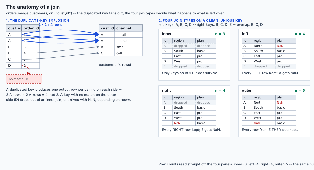
Now look at the architecture diagram below. Six order rows come in on the left. Two of them share customer ID A, and the customer-lookup table on the right also has that same ID twice — once for an old contact channel, once for a new one. The diagram draws the fan-out explicitly: one left row does not connect to one right row, it connects to two, because that is what “match on the shared key” means when the key repeats on both sides. The four join-type panels beside it show the same six rows and the same lookup table, but with a different rule for what happens to the rows with no partner at all.

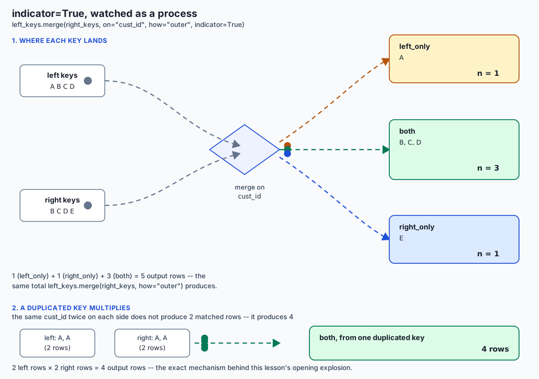
Beneath that, the animated flow diagram walks through what indicator= actually does, step by step: a key from the left table and a key from the right table travel toward each other, and depending on whether a partner shows up on the other side, the resulting row is stamped left_only, right_only, or both, with a duplicated key visibly producing more than one output row from a single pair of source rows — the shape difference the opening failure is entirely about, seen this time as a process instead of a static picture.

Historical background

pandas’ merge() function has been part of the library since very close to its beginning, and its design was deliberately modeled on SQL joins — Wes McKinney has written and spoken about pandas’ early design goals explicitly citing SQL’s JOIN semantics as the reference point for merge()’s how= argument, which is why pandas uses exactly the same four names — inner, left, right, outer — that SQL’s JOIN clauses use, rather than inventing new terminology. That choice mattered: anyone who already knew SQL joins could carry that mental model directly into pandas with almost no translation, which was a deliberate design decision to lower the barrier for the R and SQL users pandas was originally trying to win over from spreadsheets and database tools.

validate= is a considerably newer addition — it landed in pandas 0.21 (2017), years after merge() itself, in direct response to exactly the failure this lesson opens with: users merging on keys they believed were unique, getting a silently exploded result, and having no way to catch the mistake except noticing an implausible row count after the fact. The pandas maintainers added validate= as an explicit, opt-in cardinality check rather than making uniqueness checking the default behavior, for a straightforward reason — checking uniqueness costs time on every merge, including the overwhelming majority where it was never in doubt, and changing the default would have been a breaking change for a huge amount of existing code that relied on merge’s Cartesian-product behavior on purpose (a genuine many-to-many join, for instance, is completely valid and used routinely).

melt and pivot trace back to a distinction R users will recognize immediately: R’s reshape2 and later tidyr packages popularized the terms “wide” and “long” data and the melt/cast (later gather/spread, later pivot_longer/pivot_wider) vocabulary years before pandas existed in anything like its current form, and pandas’ own melt function name is a direct, acknowledged borrowing from reshape2::melt(). pivot_table, separately, borrows its name and its cross-tabulation behavior from the spreadsheet feature of the same name that predates both R and pandas by decades — Microsoft Excel’s PivotTable feature dates to the early 1990s, and pandas’ pivot_table was built explicitly to give that same aggregate-and-cross-tabulate workflow to people working in code instead of a spreadsheet grid.

The version installed for this lesson, checked directly:

>>> import pandas; pandas.__version__
'3.0.5'

What it is — and what it is not

merge(), concat(), melt() and pivot()/pivot_table() are pandas’ four tools for changing which table a piece of data lives in and which axis of a table it sits on. They are not the same operation wearing different names, and confusing them is the single most common reshaping mistake beginners make.

merge combines two different tables by matching on shared key values. It is the tool for “this row over here is about the same entity as that row over there — put their information together.” It is not for stacking two tables that already have the same structure; using merge to combine two months of the same sales report (same columns, disjoint rows) works only by accident, via an outer join on every column, and is both slower and more error-prone than the tool actually built for that job.

concat stacks tables along an axis, with no matching involved. It is the right tool for “these two tables have the same shape and I want them as one,” whether that means more rows (axis 0) or more columns (axis 1). It is not for combining tables where a row in one corresponds to a different row in the other by some shared identifier — that is what merge is for, and concat will happily produce nonsense (rows lined up by position, not by meaning) if you use it where a merge was needed.

melt and pivot do not combine anything. They reshape a single table between wide and long form. Nothing is added, nothing is removed, and no matching happens — every value that goes in comes back out, relocated from a column position to a row position, or back again.

pivot_table is pivot’s cousin, not its synonym: pivot reshapes; pivot_table reshapes and aggregates in the same call, which matters specifically when the reshaping alone would be ambiguous — more on exactly when that happens shortly.

Why it was created and what problems it solves

Real analysis almost never lives in one table. A company’s orders live in one system, its customer records in another, its product catalogue in a third — normalized apart for good reasons (a customer’s name should be stored once, not copied onto every order they ever placed), and joined back together only when a specific question needs both. merge is the tool that answers “give me every order alongside that order’s customer information” without duplicating the customer’s name into every row of the source data itself.

concat solves a narrower but constant problem: data that arrives in chunks. Twelve months of the same report, one file per region, one export per day — all sharing the same columns, needing to become one table before any aggregate analysis can run across the whole period or the whole footprint. concat is the tool for “I have several tables that are really pieces of one table.”

melt and pivot solve a shape mismatch between how data is naturally recorded and how it needs to be analyzed. A spreadsheet of exam scores is naturally wide — one column per subject, because that is how a human reading it wants to see it. But groupby('subject') needs subject to be a value in a column, not a column name — which means the natural, human-readable wide format is the wrong shape for almost any programmatic aggregation, and melt is the tool that fixes that mismatch without retyping a single number by hand.

How it works

merge() and the four join types, on one pair of frames

Everything below uses the same two small frames, so the differences are visible at a glance rather than buried across separate examples:

>>> left_keys
  cust_id region
0       A  North
1       B  South
2       C   East
3       D   West
>>> right_keys
  cust_id   plan
0       B  basic
1       C    pro
2       D    pro
3       E  basic

left_keys has customers A, B, C, D. right_keys has B, C, D, E. The overlap is exactly {B, C, D}.

Captured directly:

>>> left_keys.merge(right_keys, on="cust_id", how="inner").shape
(3, 3)
>>> left_keys.merge(right_keys, on="cust_id", how="left").shape
(4, 3)
>>> left_keys.merge(right_keys, on="cust_id", how="right").shape
(4, 3)
>>> left_keys.merge(right_keys, on="cust_id", how="outer").shape
(5, 3)

inner is the default and the most common choice — you almost always want rows where both sides had something to say. left is the second most common — “keep every one of my primary records, and attach whatever matches, blank if nothing does” — the shape you want for “enrich this table, don’t filter it.” right is the same operation with the frames’ roles reversed, and in practice most people just swap which frame is .merge()’s subject and use left instead of ever calling right explicitly. outer is for auditing: “show me everything from both sides, including what didn’t match anywhere,” which is precisely how the next section’s indicator= becomes useful.

validate=

validate= accepts four strings, each stating a claim about how many times a key may repeat on each side: "one_to_one" (neither side repeats), "one_to_many" (the left side does not repeat), "many_to_one" (the right side does not repeat), and "many_to_many" (no check at all — this is the default behavior with no validate= argument, spelled out explicitly). State the claim that matches what you actually believe about your data, and pandas checks it before merging:

>>> left_dup.merge(right_dup, on="cust_id", how="inner", validate="one_to_one")
Traceback (most recent call last):
    ...
pandas.errors.MergeError: Merge keys are not unique in either left or
right dataset; not a one-to-one merge.

left_dup has customer A three times; right_dup has customer A twice. Either fact alone breaks "one_to_one", and the error tells you which side (or both) had the problem. On genuinely unique keys, the same call raises nothing:

>>> left_keys.merge(right_keys, on="cust_id", how="inner", validate="one_to_one")
  cust_id region   plan
0       B  South  basic
1       C   East    pro
2       D   West    pro

Say this plainly, because it is the day’s single most valuable habit: validate= should be on essentially every merge you write. The cost is one keyword argument. The benefit is catching a row-count bug at the exact line that introduced it, in a stack trace that points at the merge itself, instead of three reports downstream where the wrong total looks like a business anomaly rather than a code defect.

indicator=True

Adding indicator=True appends a _merge categorical column recording, for every output row, whether it came from the left frame only, the right frame only, or both:

>>> left_keys.merge(right_keys, on="cust_id", how="outer", indicator=True)
  cust_id region   plan      _merge
0       A  North    NaN   left_only
1       B  South  basic        both
2       C   East    pro        both
3       D   West    pro        both
4       E    NaN  basic  right_only
>>> _["_merge"].value_counts()
_merge
both          3
left_only     1
right_only    1

Now reconcile, the same habit Day 123 built for groupby: left_only (1) plus both (3) must equal left_keys’ own row count (4) — it does. right_only (1) plus both (3) must equal right_keys’ own row count (4) — it does. And all three categories together must equal the merged row count (5) — they do. indicator=True is how you get the numbers to check that reconciliation against; without it you would have the merged table but no direct way to see how many rows came from where.

The silent dtype-mismatch join

Here is a trap that costs nothing to demonstrate and everything to debug in production: a key column read as int64 on one side and the same digits stored differently on the other. This is Day 121’s type-inference traps arriving with real consequences — a CSV read one way and a database column read another way can produce keys that print identically and never match.

>>> int_keyed["id"].dtype
dtype('int64')
>>> plain_str_keyed["id"].dtype
str
>>> int_keyed.merge(plain_str_keyed, on="id", how="inner")
Traceback (most recent call last):
    ...
ValueError: You are trying to merge on int64 and str columns for key
'id'. If you wish to proceed you should use pd.concat

That is an honest correction worth stating directly, because it contradicts what older pandas documentation and tutorials say happens here: on pandas 3.0.5, merging an int64 key against a plain string key does not silently return zero rows — it raises a clear ValueError that names both dtypes and tells you what to do next. This appears to be a genuine, welcome safety improvement in pandas’ more recent merge implementation, verified directly against this exact pandas version rather than assumed from older material.

The trap has not disappeared, though — it has moved. A key stored as a pandas categorical slips past that same check:

>>> cat_keyed["id"].dtype
category
>>> int_keyed.merge(cat_keyed, on="id", how="inner").shape
(0, 3)

Zero rows. No exception. No warning. This is exactly the classic failure mode, reproduced faithfully — it has simply narrowed from “any string- like key” to “a categorical key” specifically, which is precisely what you get from reading a column with dtype="category", a common and reasonable-looking choice when loading a CSV with a small number of repeated string values. The fix is the same either way — check the dtypes before you trust a join, and cast explicitly:

>>> fixed = cat_keyed.astype({"id": "int64"})
>>> int_keyed.merge(fixed, on="id", how="inner").shape
(3, 3)

on versus left_on/right_on, index joins, and suffixes

on="key" is shorthand for “the join column has the same name on both sides.” When it doesn’t, name each side explicitly:

>>> price_left.merge(renamed_right, left_on="sku", right_on="sku_code", how="inner")

.join() is merge’s sibling for joining on the index rather than a column — set the index first, then join:

>>> price_left.set_index("sku").join(price_right.set_index("sku"), how="inner", lsuffix="_l", rsuffix="_r")

Under the hood .join() calls merge() with left_index=True, right_index=True; it exists as a convenience for the very common case where the key already is the index (which Day 120 taught is where a key column often belongs anyway).

suffixes= controls what happens when both frames have a non-key column with the same name. The default is ("_x", "_y"), and it is worth seeing exactly how unhelpful that default is in practice:

>>> price_left.merge(price_right, on="sku", how="inner")
  sku  price_x  price_y
0  X1     9.99    10.99
1  X2    14.50    13.00
2  X3     3.25     3.75

price_x is the catalogue price. price_y is the live price. Neither name says so — and price_x is exactly the column name that ends up committed to a report, a dashboard, or a downstream model with no one remembering, six months later, which of _x or _y was which. This is how price_x ends up in production. Name the suffixes explicitly instead:

>>> price_left.merge(price_right, on="sku", how="inner", suffixes=("_catalog", "_live"))
  sku  price_catalog  price_live
0  X1           9.99       10.99
1  X2          14.50       13.00
2  X3           3.25        3.75

concat: axis 0, axis 1, and alignment

pd.concat([...], axis=0) stacks rows. pd.concat([...], axis=1) stacks columns. Both align by label — Day 120’s index-alignment rule, applied here across whole frames instead of within one — and fill whatever doesn’t line up with NaN, rather than raising:

>>> frame_a
   a  b
0  1  3
1  2  4
>>> frame_b
   b  c
0  5  7
1  6  8
>>> pd.concat([frame_a, frame_b], axis=0, ignore_index=True)
     a  b    c
0  1.0  3  NaN
1  2.0  4  NaN
2  NaN  5  7.0
3  NaN  6  8.0

frame_a has no c column, so its two rows get NaN there. frame_b has no a column, so its two rows get NaN there. b is present in both, so it is populated all the way down — and notice that a and c are now float64 even though every real value in them is a whole number, because a column can’t hold both integers and NaN in the same int64 array; pandas upcasts to float64 to make room for the missing values, the same widening rule Day 120 covered for a Series with a gap in it.

Along axis=1, the same alignment happens on the index instead of column names:

>>> pd.concat([frame_a2, frame_b2], axis=1)
       x     y
r1  10.0   NaN
r2  20.0  30.0
r3   NaN  40.0

r1 exists only in frame_a2, so its y is NaN. r3 exists only in frame_b2, so its x is NaN. r2 is in both, so both columns are populated.

Wide versus long: melt and pivot

A wide student-scores table, melted to long form and pivoted back:

>>> wide
   student_id  math  reading  science
0           1    88       91       76
1           2    72       85       90
2           3    95       79       83
>>> long = wide.melt(id_vars="student_id", var_name="subject", value_name="score")
>>> long.shape
(9, 3)
>>> long.pivot(index="student_id", columns="subject", values="score")
subject     math  reading  science
student_id
1             88       91       76
2             72       85       90
3             95       79       83

Long form is what groupby('subject') wants directly — “group by subject” is a groupby on a column, and in wide form, subject is not a column value at all, it’s three separate column names. The same fact applies to most plotting libraries: a “color by subject” chart wants one row per (student, subject, score) triple, which is exactly long form.

pivot versus pivot_table

pivot reshapes. It refuses to guess what to do when more than one value would land in the same cell:

>>> dup_index_col
  student  subject  score
0     Ann     math   80.0
1     Ann  reading   91.0
2      Bo     math   70.0
3     Ann     math   90.0
>>> dup_index_col.pivot(index="student", columns="subject", values="score")
Traceback (most recent call last):
    ...
ValueError: Index contains duplicate entries, cannot reshape

Ann has two math scores — 80 and 90 — and pivot has nowhere to put both in one cell, so it raises rather than picking one arbitrarily or silently overwriting one with the other. pivot_table solves the same layout problem by aggregating instead of refusing:

>>> dup_index_col.pivot_table(index="student", columns="subject", values="score", aggfunc="mean")
subject   math  reading
student
Ann       85.0     91.0
Bo        70.0      NaN

Ann’s math cell is now 85.0 — the mean of 80 and 90 — computed automatically because aggfunc="mean" (the default) told pivot_table exactly what to do with a collision. Knowing which of these two functions you want is the difference between an error that stops you and asks a question, and a silently averaged number that looks perfectly reasonable and is quietly built on two different facts merged into one.

stack and unstack

stack() and unstack() are melt and pivot’s cousins for a MultiIndex — Day 123 built one with multi-key groupby. stack() moves the innermost column level down into the row index, making the frame taller and narrower; unstack() does the reverse, moving the innermost row index level out into columns, making it wider and shorter:

>>> multi = wide.set_index("student_id")[["math", "reading"]]
>>> multi.stack()
student_id
1           math       88
            reading    91
2           math       72
            reading    85
3           math       95
            reading    79
dtype: int64
>>> multi.stack().unstack()
       math  reading
1        88       91
2        72       85
3        95       79

They are the low-level primitives pivot and unstack are partly built from — reach for melt/pivot when you are thinking in named columns, and stack/unstack when you already have a MultiIndex and want to move one of its levels between rows and columns directly.

An everyday analogy

Picture a wedding’s seating chart being built from two separate lists: a guest list (name, dietary restriction) and a table-assignment list (guest name, table number). Merging them is exactly what a data merge is — match each guest to their table by the shared key, their name.

If every guest appears exactly once on each list, this works perfectly: one taped-together card per guest, giving the caterer a table number alongside every dietary need. But suppose one guest — call her Priya — appears twice on the guest list, once under “Priya Patel” and once because someone also typed in her dietary update as a second row without realizing it was a duplicate, not a correction. And suppose the seating list also has Priya listed at two different tables, because an earlier seating draft was never fully overwritten. Merge those two duplicated Priyas against those two duplicated table assignments, and you get four place cards for Priya — one for every combination of her two guest-list entries and her two table assignments — at a wedding that has exactly one Priya and needs exactly one place card. The caterer now has two extra meals to prepare that no one will eat, and worse, if the dietary information differed between Priya’s two guest-list entries, the extra cards might even disagree with each other about what she can eat.

validate="one_to_one" is the seating coordinator’s rule, stated out loud before anyone starts taping cards together: “if either list has the same guest name twice, stop and tell me before you print anything.” It would have caught both of Priya’s duplicates at the moment the two lists were compared, not at the moment the extra place cards showed up on the table.

indicator=True is the coordinator handing back a note with every finished card: this one matched a name on both lists; this one was on the guest list but never got a table (better find out why before the wedding); this one has a table assignment for a name that isn’t on the guest list at all (an uninvited plus-one, or a data-entry error — worth checking which). And the four join types are four different instructions for what the coordinator does with a guest who has no table, or a table assignment with no matching guest: leave them off the final chart entirely (inner), keep every guest and print “table not yet assigned” for the ones missing an assignment (left), keep every table assignment and print “guest not yet identified” for the ones missing a name (right), or print everyone from both lists no matter what (outer) — the version you’d actually want the week before the wedding, precisely because it surfaces every mismatch rather than hiding any of them.

Examples in practice

A retail analytics team joins a hundred thousand order rows against a customer dimension table to compute customer lifetime value. The customer table has one row per customer — except that a recent import accidentally appended a duplicate row for roughly two thousand customers with slightly stale contact information. Without validate=, the merge silently doubles the order rows for those two thousand customers, and every downstream customer-lifetime-value figure for them is roughly twice its true value — a bias that would have been caught in seconds by validate="many_to_one" (many orders, one customer row) raising a MergeError naming the exact duplicated customer IDs.

A data engineer stitches together twelve monthly CSV exports of the same report into one year of data with pd.concat, axis=0, and discovers that one month’s export has an extra column a vendor added mid-year without telling anyone. concat’s alignment behavior means this does not break the combine — the eleven months without that column simply get NaN there — but it is exactly the kind of silent gap indicator=-style thinking should prompt a check for: is that column’s presence-or-absence meaningful, or is it noise to drop before analysis?

A machine-learning engineer builds a wide feature table — one row per user, one column per feature — for a model that expects long-form input (user ID, feature name, feature value) for a feature store’s ingestion API. melt converts the wide table in one call, without writing a loop or a manual reshape, and the round trip back through pivot is exactly how the engineer double-checks that no feature silently disappeared or duplicated in the conversion.

Implications: security, privacy, performance, scalability, and cost

Performance and scalability. A merge’s cost scales with its output size, not its input size — the opening failure’s ten-thousand-row result from two hundred input rows is not merely a correctness problem, it is a 50x performance and memory cost nobody asked for. On real production data with millions of rows per side, an unintended many-to-many merge can turn a query that should finish in seconds into one that exhausts memory entirely. validate= doubles as a cheap safety check against exactly this cost, catching it before the expensive computation runs rather than after.

Correctness and downstream trust. A merge exploded silently by a duplicated key does not merely produce more rows — it duplicates every value on the other side proportionally, which means every sum, mean, and count computed afterward is systematically inflated for the affected keys specifically, not uniformly across the dataset. That is a particularly dangerous kind of wrong, because it looks like ordinary variation between customers or categories rather than an obvious global error.

Security and privacy. Joining datasets is one of the most common ways sensitive information ends up somewhere it should not be — a table believed to be de-identified can become re-identifiable the moment it is merged against an auxiliary dataset that shares even a partial key (ZIP code plus birth date plus gender is a famous, well-studied example of near-unique re-identification from supposedly anonymous fields). Every merge is worth a brief second look at whether the combined table now carries information neither source table did on its own.

Cost. Beyond raw compute, an exploded join inflates any billed downstream cost that scales with row count — a cloud data warehouse charging per row scanned, an API call made once per row in a loop, a storage bill for a materialized result that is fifty times larger than the source data justified. validate= and a habit of checking shapes before and after a merge are close to free; the costs they prevent are not.

Alternatives: free, open source, and commercial

A database enforces key constraints that pandas cannot. This is worth stating as its own point, not folded into the table above: a SQL UNIQUE constraint on a customer ID column rejects a duplicate insert at write time, before it can ever corrupt a downstream join. pandas’ validate= only checks a merge after the duplicate is already sitting in a DataFrame — it is a safety net at read time, not a guarantee at write time. If referential integrity genuinely matters for a dataset — if a duplicated key would represent real data corruption rather than a legitimate one-to-many relationship — the join, and the constraint that protects it, probably belongs in the database, not in pandas. This lesson’s lab was run entirely with pandas and sqlite3, both installed in this environment; matplotlib, scipy and polars are not installed here, and no output from any of the three is claimed.

Comparison with related concepts

groupby (Day 123) belongs in a mental comparison here too, even though it isn’t a reshaping operation itself: groupby(...).agg(...) and pivot_table solve overlapping problems — both aggregate — but pivot_table additionally reshapes the result into a cross-tabulation (one key on the rows, another on the columns), while a plain groupby leaves every grouping key on the same axis (typically the index). pivot_table is, under the hood, close to groupby plus unstack.

When to use it — and when not to

Use merge whenever two tables describe different aspects of the same real-world entities and you need both aspects together for one analysis — and add validate= the moment you have any belief at all about how the keys should repeat, which is almost always. Use concat when you have several tables that are genuinely pieces of the same logical table, arriving in separate files or separate time periods. Use melt when your data is recorded wide (one column per category) but you need to group, filter, or plot by that category, which requires it to be a value in a column rather than a column name. Use pivot when you need a cross-tabulation and you are certain each row/column combination is unique; reach for pivot_table the moment you are not certain of that, or you explicitly want an aggregate rather than an error.

Do not reach for merge to combine data that has no real relationship — if two tables share no meaningful key, concatenating or simply keeping them separate is more honest than forcing a join on a coincidental column name. Do not skip validate= on a merge feeding anything a business decision, a report, or a model will depend on — the cost of adding it is one keyword; the cost of skipping it, on the data this lesson opened with, is a report that is fifty times too large and looks completely plausible. Do not reach for pivot on data you have not checked for duplicate index/column pairs — if you are not certain, start with pivot_table and an explicit aggfunc, and switch to pivot only once you’ve confirmed the uniqueness pivot requires.

Knowledge check

The eight questions for this lesson live in quiz.yml beside this file, covering the explosion, validate=, indicator=, the dtype-mismatch join, the four join types, concat alignment, and the pivot/ pivot_table distinction. Take it after the hands-on exercise below, not before — every question is answerable directly from something you will have run yourself by then.

Hands-on exercise

Complete “Joins That Keep Their Shape” in this lesson’s lab. Nine numbered exercises, each asserting exact row counts and exact values against small, hand-built tables you can read in full inside data.py: the merge explosion and its per-key row-count product; validate= raising and passing; indicator=True’s three counts reconciling with the inputs; the dtype-mismatch join, both its silent and its now-loud forms; all four join types on one pair of frames; the default _x/_y suffixes versus explicit ones, plus on= versus left_on=/right_on= and .join() on an index; concat’s exact NaN placement on both axes; a full melt-then-pivot round trip; and pivot raising where pivot_table aggregates instead.

Expected output

$ bash tests/run_tests.sh
...
13 checks, 0 failure(s)

pytest examples ends with 22 passed; pytest starter, on an untouched checkout, ends with 22 skipped — every exercise still has its pytest.skip(...) line in place until you replace it.

Validate your work

cd labs/sections/math-statistics-and-data/day-124-merging-and-reshaping
python3 -m venv .venv
.venv/bin/pip install -r requirements/requirements.txt
.venv/bin/pytest starter -v -k test_1   # repeat through test_9
bash tests/run_tests.sh; echo "exit=$?"

An untouched starter/ reports 22 skipped, not zero failures — a skip means “not attempted,” and the harness treats an all-skip run as incomplete work, not passing work. You are finished when pytest starter -q reports 22 passed and bash tests/run_tests.sh reports 13 checks, 0 failure(s) with exit code 0.

Troubleshooting

The lab’s troubleshooting.md covers every message you are likely to see, grouped by the exact text pandas prints — from pytest examples starter aborting on a shared module name, to a MergeError whose message doesn’t immediately say which validate= mode failed, to a melt/pivot round trip that’s off by a column order.

Common mistakes

• Trusting a merge’s row count without checking it. The fix this entire lesson teaches: look at input and output shapes, every time, and reach for validate= the moment you have any belief about cardinality.
• Reading _x/_y as meaningless noise instead of a warning sign. Seeing those suffixes in your own output means you have not named your suffixes= yet, on columns you should probably be able to tell apart.
• Assuming a dtype mismatch always raises. Exercise 4 proves both halves of the truth on pandas 3.0.5: a plain string key against int64 now raises ValueError, but a categorical key against int64 still fails silently, with zero rows and no exception at all.
• Forgetting pivot requires uniqueness pandas will not manufacture for you. If your index/column pair might repeat, start with pivot_table and a chosen aggfunc, not pivot.

Practice assignment

Take any two small tables you have on hand — even two CSVs of ten rows each will do — and deliberately introduce one duplicated key value into each. Merge them without validate= and record the row count. Add validate="one_to_one" and confirm it raises. Then add indicator=True to an outer merge of the same two tables and write, in one paragraph, what each of the three _merge categories tells you about your specific data that the row count alone would not have.

Extension challenge

Build a small “orders” table and a “customer lookup” table where the lookup table has exactly one customer ID duplicated by accident — the realistic version of this lesson’s opening failure. Compute total revenue per customer two ways: once from a plain merge with no validate=, and once after catching and fixing the duplicate with validate=. Report the exact dollar amount the unvalidated version overstated for the affected customer, and write one paragraph connecting that number to this lesson’s AI thread below — specifically, what an over-weighted, duplicated entity would do to a model trained on the unvalidated version of that table.

AI thread

Feature engineering is, more often than most people realize, mostly joins. A user’s demographic features, their behavioral history, their account metadata, a third-party enrichment table — a real feature pipeline stitches all of it together from separate sources, and every one of those stitches is a merge with exactly the cardinality risk this lesson opened with. A duplicated key in a lookup table is one of the quietest ways to corrupt a training set, because the corruption is not random noise a model can learn to ignore — it is a systematic over-representation of specific entities. If a lookup table has one customer duplicated three times, every training example involving that customer is effectively triplicated, and the model does not experience that as “here is one customer’s pattern, stated three times as strongly as it should be.” It experiences it as three independent pieces of evidence, and it learns that customer’s particular quirks — including whatever noise happens to be in their specific records — more strongly than the evidence actually justifies. At evaluation time, this can produce a model that looks like it’s performing well, because it has effectively memorized the over-weighted, duplicated entities, while generalizing worse than reported to everyone else. validate= costs one argument and catches this at the point where the corrupted feature table is built — the cheapest possible place to catch it, and immeasurably cheaper than discovering it three months later as an unexplained fairness gap or a stubborn evaluation-versus-production performance mismatch that no one can quite trace back to its source.

Quiz

Glossary

merge

The pandas operation that combines two DataFrames by matching rows on one or more shared key values, analogous to a SQL JOIN. Every left row is paired with every right row sharing its key, which is why a duplicated key on both sides produces a per-key Cartesian product rather than a one-to-one pairing.

cardinality (of a join)

A claim about how many times a merge key may repeat on each side of a join -- for example, that a customer ID appears at most once in a customer table (one) but many times in an orders table (many). validate= turns a stated cardinality claim into an enforced check that pandas performs before completing the merge.

validate

A merge() keyword accepting "one_to_one", "one_to_many", "many_to_one" or "many_to_many", each stating a cardinality assumption about the merge key on each side. If the assumption is false, pandas raises pandas.errors.MergeError before producing any output, rather than silently completing an unintended Cartesian product.

MergeError

The exception pandas raises when a merge's validate= argument detects that the stated cardinality assumption does not hold -- for example, validate="one_to_one" on a key that is duplicated on either side.

indicator

A merge() keyword that, when set to True, adds a categorical _merge column to the result recording whether each row's key matched on the left frame only (left_only), the right frame only (right_only), or both (both). The three counts must sum to the merged row count, and left_only plus both must equal the left frame's own row count whenever the left key has no duplicates.

how (join type)

The merge() keyword selecting inner (keep only matching keys), left (keep every left row), right (keep every right row), or outer (keep every row from both sides), filling NaN wherever no match exists on the kept side. Named identically to SQL's JOIN clauses, which pandas' merge design deliberately mirrors.

suffixes

A merge() keyword controlling what gets appended to a non-key column name that appears in both input frames. Defaults to ("_x", "_y"), which is how an uninformative column name like price_x ends up in a merged result unless suffixes= is passed explicitly.

left_on / right_on

merge() keywords naming the join column on the left frame and the right frame separately, used when the two frames' key columns have different names. on= is shorthand for the common case where both sides share the same column name.

join (DataFrame method)

A DataFrame method that merges on the index rather than a column, calling merge() internally with left_index=True and right_index=True. Convenient when the join key already is a table's index.

concat

The pandas function that stacks DataFrames along an axis -- axis=0 adds rows, axis=1 adds columns -- without matching on any key. Aligns by column name (axis=0) or index label (axis=1), filling any position that does not line up across the inputs with NaN rather than raising an error.

wide format

A table layout with one column per measurement or category -- for example, separate math, reading and science score columns for each student. Natural to read but usually the wrong shape for groupby-based aggregation or most plotting libraries.

long format

A table layout with one row per individual measurement, carrying a column naming which measurement it is and a column holding its value. The shape groupby, most aggregation functions, and most plotting libraries expect a categorical variable to be in.

melt

The DataFrame method that converts a table from wide format to long format, turning selected column names into values of a new "variable" column and their corresponding values into a new "value" column, while keeping any id_vars columns unchanged per row.

pivot

The DataFrame method that converts long format back to wide format by placing one column's values into the row index, another column's values into the column labels, and a third column's values into the resulting cells. Raises ValueError if any index/column pair repeats, since it has nowhere to place two values in one cell.

pivot_table

pivot's aggregating cousin: reshapes long format into wide format the same way pivot does, but resolves a duplicate index/column pair by applying an aggregation function (aggfunc, "mean" by default) instead of raising an error.

stack / unstack

DataFrame methods that move a level of a MultiIndex between the row index and the column labels. stack() moves the innermost column level down into the row index, making the frame taller; unstack() moves the innermost row-index level out into columns, making it wider.

dtype-mismatch join

A join failure caused by the same key values being stored with different pandas dtypes on each side -- for example, int64 on one side and a pandas Categorical of the same digits on the other. On pandas 3.0.5, an int64-versus-categorical mismatch returns zero matching rows silently, while an int64-versus-plain-string mismatch raises ValueError instead.

Sources and further reading

• Merge, join, concatenate and compare — pandas Development Team (accessed 2026-08-19)
• Reshaping and pivot tables — pandas Development Team (accessed 2026-08-19)
• pandas.DataFrame.merge — pandas Development Team (accessed 2026-08-19)
• Indexing and selecting data — pandas Development Team (accessed 2026-08-19)
• sqlite3 -- DB-API 2.0 interface for SQLite databases — Python Software Foundation (accessed 2026-08-19)

Mark Day 124 as read
Kept in this browser, no account needed. Your progress page turns the whole record into one link you can bookmark or open on another device.