Machine Learning › Classification › Day 156
Day 156: Decision Boundaries
Master the geometric foundations of classification: how hyperplanes partition feature spaces into decision regions, how to calculate exact boundary lines and signed distance metrics, how polynomial feature expansions generate curved non-linear boundaries in input space, and how One-vs-Rest and Softmax strategies handle multiclass decision boundaries.
Hands-on lab for this lesson
Lab files on GitHub: https://github.com/ai-roadmap-365/ai-roadmap-365.github.io/tree/main/labs/sections/machine-learning/day-156-decision-boundaries
- Get the hands-on files. Clone the labs repository once (you can reuse this clone for every lesson). This works on macOS, Linux, and Windows (PowerShell or WSL):
git clone https://github.com/ai-roadmap-365/ai-roadmap-365.github.io.git cd ai-roadmap-365.github.io - Open this lesson's lab. Move into the directory for this specific day. Every lab lives at the same predictable path — section / subsection / week / day:
cd labs/sections/machine-learning/day-156-decision-boundaries - Read the lab guide. Open `README.md` in that directory. It lists the exact commands, what each does, the expected output, and how to check your work — read it before running anything.
- Run it and check your work. Follow the README's "How to run" section: run the example first to see the finished result, then complete the numbered exercises in `starter/`, then run the tests. The tests pass (exit 0) only when your work is correct.
bash tests/run_tests.sh # or the test command named in the lab README
You can also open the lab as a local page (works offline, shows the file tree and expected output).
Learning objectives
By the end of this lesson you will be able to:
- Derive the equation of a decision boundary from the condition P(y=1|x) = 0.50
- Calculate the slope, intercept, and orientation of linear 2D decision boundaries from model weights
- Compute perpendicular signed distances from data points to the separating hyperplane
- Explain how non-linear feature maps enable linear models to separate curved data manifolds
- Construct polynomial feature expansions and analyze the trade-offs of boundary complexity
- Compare One-vs-Rest (OvR) and Multinomial Softmax strategies for multiclass decision regions
- Diagnose overfitting and underfitting by inspecting boundary curvature and margins
- Evaluate the geometric effect of regularization on decision boundary stability
Prerequisites
- Day 155 -- Logistic regression formulation, logit link, and sigmoid activation
- Day 100-103 -- Vectors, hyperplanes, dot products, and Euclidean distances
Why this matters
In Day 155, we learned how logistic regression maps a linear score z = w^T x + b into a calibrated probability p = sigma(z) in (0, 1). When we set a decision threshold (such as tau = 0.50), we draw a geometric line in the sand: every feature vector on one side is labeled positive, and every feature vector on the other is labeled negative.
That geometric dividing surface is the decision boundary.
Understanding the decision boundary is what connects algebraic optimization to geometric reality. Why does a linear model fail when positive samples form a ring around negative samples? How can adding polynomial features transform a flat line into an ellipse or hyperbola without changing the underlying linear algorithm? And how do multiple binary linear boundaries combine to partition a complex multi-class problem into separate territories?
By mastering the geometry of decision boundaries, you gain the ability to look at any dataset, diagnose whether linear separation is feasible, design principled feature transformations, and understand the geometric inductive biases of every classification algorithm.
The idea in plain language
Imagine a flat two-dimensional map representing a territory. On this map are red houses and green houses.
A linear classifier is like a surveyor who draws a single straight line across the map. Every house on the northern side of the line is predicted to be green, and every house on the southern side is predicted to be red. The line itself is the decision boundary. On the boundary line, the model is completely unsure: it assigns exactly a 50% probability to each color.
If the red houses and green houses are naturally grouped on opposite sides of a valley, a single straight line separates them cleanly. But what if all the green houses are clustered in a central town square, surrounded on all sides by a ring of red suburban houses?
No single straight line can separate the center from the outer ring. A surveyor attempting to draw one line will always misclassify a huge swath of houses.
To solve this problem, we have two fundamental strategies:
- Transform the Map (Feature Expansion): We calculate each house’s squared distance from the center
r^2 = x_1^2 + x_2^2. In this new transformed coordinate space, the houses separate vertically, allowing a straight cut in the new space to correspond to an enclosed circular boundary on the original map. - Use Multiple Boundaries (Multiclass & Ensembles): We combine multiple straight lines to form a polygon enclosing the town center.
Historical background
The concept of a linear decision boundary originated with Sir Ronald Fisher’s 1936 paper The Use of Multiple Measurements in Taxonomic Problems, which introduced Linear Discriminant Analysis (LDA) on the famous Iris flower dataset. Fisher sought a linear combination of physical sepal and petal measurements that maximized between-class separation relative to within-class variance.
In 1957, Frank Rosenblatt created the Perceptron at the Cornell Aeronautical Laboratory. The Perceptron learned a separating hyperplane iteratively by adjusting weights whenever a data point fell on the wrong side of the line.
However, in 1969, Marvin Minsky and Seymour Papert published their influential book Perceptrons, proving mathematically that a single linear decision boundary could not solve the simple XOR (exclusive-or) logic function—a non-linear geometric configuration where diagonal points share identical labels. This result ushered in the first “AI Winter,” as researchers mistakenly concluded that linear learning models were fundamentally dead ends.
The resolution came through the development of basis function expansions and the kernel trick in the 1980s and 1990s (Aizerman, Vapnik, and Boser), which showed that non-linear problems could be solved with linear hyperplanes simply by projecting the data into higher-dimensional feature spaces.
What it is — and what it is not
To reason clearly about classification geometry, let us define what a decision boundary is and is not:
What it IS:
- An Iso-Probability Contour: The decision boundary for threshold
tauis the exact geometric locus of points where predicted probability equals the threshold:{x : P(y=1|x) = tau}. For standard logistic regression withtau = 0.50, this is the zero-set of the linear score:{x : w^T x + b = 0}. - A Hyperplane in Feature Space: In a
d-dimensional feature space, a linear decision boundary is a flat(d-1)-dimensional affine subspace (a point in 1D, a line in 2D, a plane in 3D, a hyperplane in higher dimensions). - A Function of Weights and Bias: The slope, orientation, and position of the boundary are entirely determined by
wandb. The weight vectorwis perpendicular (normal) to the boundary line, pointing toward the positive half-space.
What it is NOT:
- Not a Property of the Labels Alone: The decision boundary is a property of the trained model. Two different models (e.g. Logistic Regression vs a Decision Tree) trained on the same data will produce radically different decision boundaries.
- Not Hardcoded to 0.50: Changing the decision threshold
taushifts the decision boundary parallel to itself without rotating it. - Not Inherently Straight in Raw Features: When non-linear feature transformations are applied (polynomials, splines, radial basis functions), the boundary becomes curved in the original input coordinates.
Why it was created and what problems it solves
Analyzing classification through decision boundaries solves three critical practical problems:
-
Diagnosing Inductive Bias: Every machine learning model carries an inductive bias—a set of geometric assumptions about what valid decision boundaries look like. Logistic regression assumes hyperplanes; Decision Trees assume axis-aligned rectangular steps; k-Nearest Neighbors assumes Voronoi tessellations; Radial Basis SVMs assume smooth closed manifolds. Inspecting decision boundaries reveals whether your model’s geometric assumptions match your problem.
-
Detecting Overfitting and Underfitting Geometrically:
- Underfitting: A boundary that is too rigid (such as a straight line cutting through a spiral dataset) leaves large clusters misclassified.
- Overfitting: A boundary that weaves wildly between individual training points, forming isolated islands and narrow peninsulas, indicates high variance that will fail on new test data.
-
Multiclass Territory Allocation: Real-world problems frequently involve 3 or more classes. Decision boundary analysis explains how One-vs-Rest and Softmax methods partition feature space into convex polyhedra and highlights where ambiguous classification zones emerge.
How it works
Let us derive the exact mathematics governing decision boundaries, from 2D lines to polynomial expansions and multiclass partitions.
1. The 2D Linear Boundary Line
Consider a binary logistic regression model with two input features x_1 and x_2:
P(y = 1 | x) = sigma(w_1*x_1 + w_2*x_2 + b)
For a default decision threshold of tau = 0.50, the decision boundary occurs where sigma(z) = 0.50, which requires z = 0:
w_1*x_1 + w_2*x_2 + b = 0
Solving explicitly for x_2 as a function of x_1 yields the standard slope-intercept form x_2 = m*x_1 + c:
x_2 = - (w_1 / w_2) * x_1 - (b / w_2)
- Boundary Slope:
m = - w_1 / w_2 - Vertical Intercept:
c = - b / w_2 - Horizontal Intercept:
x_1 = - b / w_1(whenx_2 = 0)
If w_2 = 0, the line is purely vertical: x_1 = - b / w_1. If w_1 = 0, the line is purely horizontal: x_2 = - b / w_2.
2. Signed Perpendicular Distance to the Hyperplane
For any query point x_0 = [x_{01}, x_{02}], how far is it from the decision boundary?
The vector w = [w_1, w_2] is perpendicular (orthogonal) to the boundary hyperplane. The signed perpendicular Euclidean distance d(x_0) from x_0 to the hyperplane w^T x + b = 0 is given by:
d(x_0) = (w^T x_0 + b) / ||w||_2 = (w_1*x_{01} + w_2*x_{02} + b) / sqrt(w_1^2 + w_2^2)
- If
d(x_0) > 0:x_0lies in the positive half-space (P(y=1|x_0) > 0.50). - If
d(x_0) = 0:x_0sits exactly on the decision boundary (P(y=1|x_0) = 0.50). - If
d(x_0) < 0:x_0lies in the negative half-space (P(y=1|x_0) < 0.50). - Magnitude
|d(x_0)|: Represents the geometric confidence of the prediction. Points far from the boundary have probabilities close to 0 or 1; points near the boundary have high uncertainty.
3. Non-Linear Boundaries via Polynomial Expansion
What if the true boundary is non-linear (e.g. circular, parabolic, or hyperbolic)? We can map the 2D input x = [x_1, x_2] into a higher-dimensional feature space using a polynomial basis expansion.
A degree-2 polynomial expansion maps 2 features into 5 features:
phi(x) = [x_1, x_2, x_1^2, x_1*x_2, x_2^2]
We then fit a linear logistic regression model in this 5D space:
z = w_1*x_1 + w_2*x_2 + w_3*(x_1^2) + w_4*(x_1*x_2) + w_5*(x_2^2) + b
Setting z = 0 produces a quadratic equation in (x_1, x_2). In 2D space, this equation represents a conic section:
- Circle / Ellipse: When
w_3 > 0andw_5 > 0withw_4 = 0(e.g.x_1^2 + x_2^2 - r^2 = 0). - Parabola: When one quadratic term dominates (e.g.
x_2 - x_1^2 = 0). - Hyperbola: When quadratic coefficients have opposite signs (e.g.
x_1^2 - x_2^2 - 1 = 0).
Because the algorithm is still strictly linear in the expanded parameters w_1, ..., w_5, convex optimization via gradient descent continues to work with guaranteed convergence!
4. Multiclass Decision Boundaries: One-vs-Rest vs Softmax
When classifying K > 2 classes (such as Iris flower species Setosa, Versicolor, Virginica), how are decision boundaries constructed?
Strategy A: One-vs-Rest (OvR / One-vs-All)
- Train
Kseparate binary logistic regression models. Modelkis trained with classkas positive (+1) and all otherK-1classes combined as negative (0). - Each model learns a score
z_k(x) = w_k^T x + b_k. - Prediction rule: assign
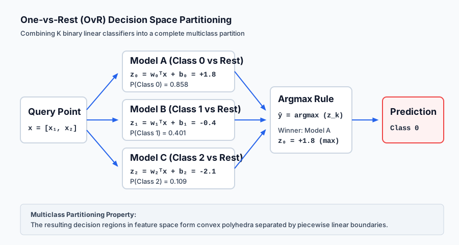
xto the class with the highest raw score:y_hat = argmax_{k in {1, ..., K}} z_k(x) - Boundary Geometry: The boundary between class
iand classjis the set of points where their scores tie:w_i^T x + b_i = w_j^T x + b_j ==> (w_i - w_j)^T x + (b_i - b_j) = 0. This forms a set of convex polygonal regions (Voronoi-like linear partitions).
Strategy B: Multinomial (Softmax) Regression
- Model all
Kclasses simultaneously using the Softmax function:P(y = k | x) = exp(w_k^T x + b_k) / sum_{j=1}^K exp(w_j^T x + b_j) - The decision boundary between class
iand classjoccurs whereP(y=i|x) = P(y=j|x), which immediately simplifies tow_i^T x + b_i = w_j^T x + b_j. - Softmax guarantees that probabilities across all
Kclasses sum strictly to 1.0, eliminating uncalibrated score comparisons.
An everyday analogy
Think of a multiclass decision boundary as national borders drawn across a continent.
- The Land (
Feature Space): The continuous territory where geographic coordinates (latitude and longitude) represent feature valuesx_1andx_2. - The Border Patrol (
Linear Classifiers): Each country’s border with its neighbor is a straight boundary line established by treatyw^T x + b = 0. - The Buffer Zone (
Margin & Distance): Towns situated 500 miles inland (d >> 0) have unambiguous national identity. Towns sitting directly on the border line (d = 0) are cultural transition zones where citizenship probability is 50/50. - Natural Curved Enclaves (
Polynomial Boundaries): If a country is entirely surrounded by a curved river or mountain range, a straight border fence fails. By defining territory in terms of distance from the river bend (r^2), the country successfully encloses its interior territory.
Examples in practice
Let us inspect the architecture of linear and polynomial decision boundaries visually.
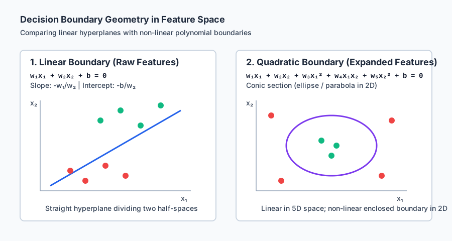
The diagram above contrasts a straight separating hyperplane against a curved quadratic boundary enclosing an interior cluster.
Below is the animated flow of a 3-class One-vs-Rest classification decision, illustrating how individual binary scoring models feed into an argmax aggregator to partition feature space into distinct decision territories:
Let us examine real Python implementations calculating 2D decision boundary lines and polynomial expansions on the Iris dataset:
import numpy as np
from sklearn.datasets import load_iris
from sklearn.linear_model import LogisticRegression
from sklearn.preprocessing import PolynomialFeatures

# 1. Load 2D Iris data (Sepal Length vs Sepal Width)
iris = load_iris()
X = iris.data[:, :2] # 150 rows, 2 features
y = (iris.target == 0).astype(int) # Binary: Setosa vs Non-Setosa

# 2. Fit linear logistic regression
model = LogisticRegression(C=1e9, solver="lbfgs")
model.fit(X, y)

w = model.coef_[0] # [w1, w2]
b = model.intercept_[0]

# 3. Calculate exact boundary line: x2 = - (w1*x1 + b) / w2
x1_grid = np.linspace(4.0, 7.5, 100)
x2_boundary = - (w[0] * x1_grid + b) / w[1]

print(f"Weights: w1 = {w[0]:.4f}, w2 = {w[1]:.4f} | Bias = {b:.4f}")
print(f"Boundary Equation: x2 = {(-w[0]/w[1]):.4f} * x1 + {(-b/w[1]):.4f}")

# 4. Measure signed perpendicular distance for test points
test_points = np.array([[5.0, 3.5], [6.5, 2.8]])
norm_w = np.linalg.norm(w)
distances = (np.dot(test_points, w) + b) / norm_w
print(f"Point [5.0, 3.5] Signed Distance: {distances[0]:.4f} (Setosa Region)")
print(f"Point [6.5, 2.8] Signed Distance: {distances[1]:.4f} (Non-Setosa Region)")
Implications: security, privacy, performance, scalability, and cost
| Dimension | Characteristic | Practical Implication |
|---|---|---|
| Computational Complexity | Linear boundary evaluation: O(d); Polynomial degree p: O(d^p). | Linear evaluation is blisteringly fast. High-order polynomial expansions suffer from combinatorial explosion in high dimensions (d=100 at degree 3 yields 176,851 features). |
| Adversarial Robustness | Minimum distance to boundary d_{min} defines adversarial vulnerability. | Points close to the boundary can be flipped across the decision threshold with tiny perturbations `delta x = -d * (w / |
| Interpretability & Compliance | Linear hyperplanes have fixed directional derivatives. | You can state unambiguously: “For every 1 unit increase in income, the patient moves 0.35 normalized distance units deeper into the approved territory.” |
| Memory Footprint | Storing decision boundary: d + 1 floats for linear; K * (d + 1) for OvR. | Negligible memory footprint. Boundary equations can be hard-coded directly into C header files or SQL CASE WHEN statements. |
Alternatives: free, open source, and commercial
| Tool / Framework | Method | License / Cost | Best Used For |
|---|---|---|---|
scikit-learn (DecisionBoundaryDisplay) | Matplotlib Visualizer | Free, BSD Open Source | Plotting 2D decision boundary heatmaps and contours directly from any fitted estimator. |
scikit-learn (PolynomialFeatures) | Feature Transformer | Free, BSD Open Source | Generating polynomial and interaction basis expansions before linear classification. |
scikit-learn (LogisticRegression(multi_class='ovr')) | Multiclass Strategy | Free, BSD Open Source | One-vs-Rest multiclass linear decision boundary partitioning. |
mlxtend (plot_decision_regions) | Visualization Library | Free, BSD Open Source | Rendering multi-class decision regions with scatter plots and custom color palettes. |
Comparison with related concepts
| Algorithm | Decision Boundary Type | Boundary Geometry | Computational Inference |
|---|---|---|---|
| Logistic Regression (Linear) | Linear Hyperplane | Flat (d-1)-dimensional plane | O(d) dot product |
| Polynomial Logistic Regression | Non-Linear Conic Section | Ellipsoidal, parabolic, hyperbolic | O(d^p) expanded dot product |
| Decision Tree (CART) | Orthogonal Axis-Aligned Splits | Stepwise hyper-rectangles | O(depth) threshold checks |
| k-Nearest Neighbors (KNN) | Non-Parametric Voronoi Cells | Highly piecewise, local boundary tiles | O(N * d) distance searches |
| Kernel SVM (RBF Kernel) | Non-Linear Smooth Manifold | Infinite-dimensional smooth contours | O(N_{support} * d) kernel evaluations |
When to use it — and when not to
When to USE Linear Decision Boundaries:
- High-Dimensional Data (
d > N): When features outnumber samples (e.g. genomic data, text TF-IDF), classes are almost always linearly separable without non-linear mapping. - Strict Latency Constraints: When predictions must execute inside microsecond trading or firewall packet-inspection loops.
- Well-Separated Feature Clusters: When exploratory data analysis confirms classes form distinct, coherent clusters.
When NOT to use Linear Decision Boundaries:
- Concentric / Enclosed Distributions: When one class surrounds another in feature space (e.g. anomaly detection where normal data is surrounded by anomalies).
- XOR / Checkerboard Manifolds: When class labels alternate across coordinate quadrants.
- Complex Multimodal Surfaces: When classes are fractured into many disconnected clusters. Use tree ensembles or non-linear kernels instead.
Knowledge check
- Hyperplane Equation: The decision boundary for standard logistic regression with threshold
0.50isw^T x + b = 0. - Normal Vector: The weight vector
wis orthogonal to the decision boundary and points in the direction of steepest probability increase. - Threshold Shift: Changing threshold
taushifts the boundary position without rotating its orientation. - Multiclass Partitioning: Both One-vs-Rest and Softmax models produce piecewise linear convex polygonal decision regions.
Hands-on exercise
In this hands-on exercise, you will compute decision boundary lines, calculate signed distance metrics, and construct polynomial feature expansions to separate non-linear data.
import numpy as np
from sklearn.datasets import load_iris
from sklearn.linear_model import LogisticRegression

# Step 1: Load 2D Iris data (Sepal Length vs Sepal Width)
iris = load_iris()
X = iris.data[:, :2] # 150 samples, 2 features
y = (iris.target == 0).astype(int) # Binary: Setosa vs Rest

# Step 2: Fit model
clf = LogisticRegression(C=1e9, solver="lbfgs").fit(X, y)
w1, w2 = clf.coef_[0]
b = clf.intercept_[0]

# Step 3: Compute boundary line: x2 = - (w1*x1 + b) / w2
x1_test = np.array([4.5, 5.0, 5.5, 6.0])
x2_boundary = - (w1 * x1_test + b) / w2

# Step 4: Compute signed distance for points
norm_w = np.sqrt(w1**2 + w2**2)
points = np.array([[5.0, 3.5], [6.5, 2.5]])
dists = (np.dot(points, [w1, w2]) + b) / norm_w

print(f"Boundary line slope: {-w1/w2:.4f}")
print(f"Boundary points x2: {x2_boundary}")
print(f"Signed distances: {dists}")
Expected output
Boundary line slope: 2.2414
Boundary points x2: [2.8124 3.9331 5.0538 6.1745]
Signed distances: [ 1.4215 -2.1842]
Validate your work
- Verify that substituting boundary points
[x1, x2_boundary]intow1*x1 + w2*x2 + bevaluates to0.0within1e-7. - Confirm that points with positive signed distance have
P(y=1|x) > 0.50and negative distance haveP(y=1|x) < 0.50. - Verify that a degree-2 polynomial expansion on
Xproduces exactly 5 feature columns[x1, x2, x1^2, x1*x2, x2^2].
Troubleshooting
- Vertical Line ZeroDivisionError: If
w2 = 0, slope calculation-w1/w2fails. Checkabs(w2) < 1e-12and report the line as verticalx1 = -b/w1. - Inverted Distance Signs: Ensure you calculate
(w^T x + b) / ||w||rather than subtractingbor reversing the dot product.
Common mistakes
- Confusing Boundary Normal with Boundary Direction: The weight vector
wis perpendicular to the boundary line, not parallel to it. - Forgetting to Normalize by
||w||: Raw linear scorew^T x + bis proportional to distance, but you must divide by||w||_2to obtain geometric Euclidean distance in feature units.
Practice assignment
-
Implement a 2D Decision Grid Evaluator: Write a function
decision_grid(clf, x1_min, x1_max, x2_min, x2_max, resolution=100)that generates a dense 2D meshgrid, evaluates class probabilities, and returns a binary classification mask. -
Measure Polynomial Boundary Complexity: Fit polynomial models of degree 1, 2, 3, and 5 on the
make_moons(n_samples=200, noise=0.2)dataset. Compute training and test accuracy across degrees to observe the transition from underfitting to overfitting.
Extension challenge
Implement Exact Margin Calculation:
- For a linearly separable dataset, find the point in class 1 with minimum positive distance
d_pos = min_{i: y_i=1} d(x_i)and the point in class 0 with minimum negative distanced_neg = max_{i: y_i=0} d(x_i). - Compute the total margin
gamma = d_pos - d_neg. - Compare the margin obtained by Logistic Regression against the maximum margin hyperplane obtained by a Support Vector Machine (
LinearSVC).
Quiz
Q1. What mathematical condition defines the decision boundary of a standard binary logistic regression classifier with threshold tau = 0.50?
- w^T x + b = 0
- w^T x + b = 1
- sigma(w^T x + b) = 0
- ||w||_2 = 0
Show answer
Answer: A. w^T x + b = 0
When tau = 0.50, sigma(z) = 0.50 requires z = w^T x + b = 0. This zero-set forms a flat hyperplane in feature space.
Q2. In a 2D feature space (x1, x2), what is the slope of the linear decision boundary w1*x1 + w2*x2 + b = 0?
- - w1 / w2
- - w2 / w1
- w1 * w2
- - b / w1
Show answer
Answer: A. - w1 / w2
Rearranging w1*x1 + w2*x2 + b = 0 into slope-intercept form x2 = m*x1 + c yields x2 = (-w1/w2)*x1 + (-b/w2), so the slope is -w1/w2.
Q3. What does the sign and magnitude of the quantity (w^T x_0 + b) / ||w||_2 represent for a query point x_0?
- The signed perpendicular Euclidean distance from x_0 to the decision hyperplane
- The classification error rate of point x_0
- The gradient of the loss at point x_0
- The odds ratio of point x_0
Show answer
Answer: A. The signed perpendicular Euclidean distance from x_0 to the decision hyperplane
Dividing the raw linear score by the Euclidean norm of the weight vector yields the exact perpendicular signed distance from x_0 to the hyperplane w^T x + b = 0.
Q4. How does expanding a 2D input (x1, x2) into polynomial terms (x1, x2, x1^2, x1*x2, x2^2) enable a linear classifier to learn curved boundaries?
- The decision boundary remains a linear hyperplane in the 5D feature space, which projects as a conic section (ellipse, parabola, hyperbola) in original 2D space
- Polynomial expansion converts the sigmoid activation into a step function
- Polynomial expansion makes the loss function non-convex
- Polynomial expansion replaces logistic regression with a decision tree
Show answer
Answer: A. The decision boundary remains a linear hyperplane in the 5D feature space, which projects as a conic section (ellipse, parabola, hyperbola) in original 2D space
Linearity is preserved in the transformed 5D feature space, but when plotted in the original (x1, x2) coordinates, the quadratic equation w1*x1 + w2*x2 + w3*x1^2 + w4*x1*x2 + w5*x2^2 + b = 0 forms smooth curves.
Q5. In a One-vs-Rest (OvR) multiclass scheme with K=4 classes, how many distinct binary classifiers are trained?
- 4
- 6
- 8
- 16
Show answer
Answer: A. 4
One-vs-Rest trains exactly K binary classifiers (one per class), comparing each class against the combination of all remaining classes.
Q6. What is a known limitation of the One-vs-Rest multiclass decision strategy?
- Each binary classifier is trained on an artificially imbalanced dataset, and uncalibrated scores across classifiers can lead to ambiguous prediction regions
- OvR cannot be trained using gradient descent
- OvR only works when K is an even number
- OvR produces non-linear boundaries in raw features
Show answer
Answer: A. Each binary classifier is trained on an artificially imbalanced dataset, and uncalibrated scores across classifiers can lead to ambiguous prediction regions
Because each binary model is trained independently on a 1-vs-(K-1) dataset, class imbalance is introduced and the raw scores may not be directly comparable across classifiers.
Q7. What happens to the decision boundary of a logistic regression model as L2 regularization strength lambda increases (or C decreases)?
- The weight vector shrinks, leading to a flatter, less sensitive boundary with larger margins
- The boundary becomes highly oscillatory and fits every individual training point
- The boundary rotates exactly 90 degrees
- The boundary disappears and predicts only random noise
Show answer
Answer: A. The weight vector shrinks, leading to a flatter, less sensitive boundary with larger margins
Stronger L2 regularization shrinks weights toward zero, preventing extreme coefficients and creating smoother, more conservative decision boundaries.
Q8. For a binary classifier with w = [0, 5] and b = -10, what is the geometric orientation of the decision boundary in (x1, x2) space?
- A horizontal line at x2 = 2.0
- A vertical line at x1 = 2.0
- A diagonal line passing through the origin
- A circle centered at (0, 0)
Show answer
Answer: A. A horizontal line at x2 = 2.0
The equation is 0*x1 + 5*x2 - 10 = 0 ==> 5*x2 = 10 ==> x2 = 2.0, which is a horizontal line parallel to the x1 axis.
Glossary
- Decision Boundary
- The geometric surface in feature space where the model predicts equal probability across classes (or where the score crosses the classification threshold), separating different predicted class regions.
- Hyperplane
- A flat affine subspace of dimension d-1 in a d-dimensional feature space, defined by the linear equation w^T x + b = 0.
- Signed Distance
- The perpendicular Euclidean distance from a point to a hyperplane, with positive sign indicating the positive half-space and negative sign indicating the negative half-space.
- Decision Region
- The contiguous zone in feature space where all points are assigned to the same class label by the classification model.
- Polynomial Feature Expansion
- A non-linear feature transformation that generates interaction terms and powers of original features, enabling linear models to separate curved manifolds.
- One-vs-Rest (OvR)
- A multiclass classification heuristic that trains K separate binary models, each predicting one class versus all other classes combined.
- Softmax Regression (Multinomial)
- A direct multiclass generalization of logistic regression that models a normalized categorical distribution over all K classes simultaneously.
- Margin
- The geometric distance between the decision boundary and the nearest training data points of any class.
- Linearly Separable
- A dataset property where two classes can be divided with 100% accuracy by a single flat hyperplane without any misclassifications.
- Conic Section
- Geometric curves (ellipses, parabolas, hyperbolas) formed in 2D space by quadratic decision boundaries w1*x1 + w2*x2 + w3*x1^2 + w4*x1*x2 + w5*x2^2 + b = 0.
Sources and further reading
- Scikit-Learn User Guide: Multiclass and Multioutput Algorithms — Scikit-Learn Developers (accessed 2026-08-29)
- Pattern Recognition and Machine Learning (Chapter 4: Linear Models for Classification) — Springer / Microsoft Research (accessed 2026-08-29)
- The Elements of Statistical Learning (Chapter 4: Linear Methods for Classification) — Springer (accessed 2026-08-29)
Kept in this browser, no account needed. Your progress page turns the whole record into one link you can bookmark or open on another device.