Machine Learning › Classification › Day 155
Day 155: Logistic Regression

Learn how to frame binary classification from first principles: why linear regression fails on binary targets, how the sigmoid function maps unbounded real numbers into calibrated probabilities, how the logit and log-odds link function operate, how Maximum Likelihood Estimation produces the binary cross-entropy loss, and how gradient descent trains a robust logistic regression model.
Hands-on lab for this lesson
Lab files on GitHub: https://github.com/ai-roadmap-365/ai-roadmap-365.github.io/tree/main/labs/sections/machine-learning/day-155-logistic-regression
- Get the hands-on files. Clone the labs repository once (you can reuse this clone for every lesson). This works on macOS, Linux, and Windows (PowerShell or WSL):
git clone https://github.com/ai-roadmap-365/ai-roadmap-365.github.io.git cd ai-roadmap-365.github.io - Open this lesson's lab. Move into the directory for this specific day. Every lab lives at the same predictable path — section / subsection / week / day:
cd labs/sections/machine-learning/day-155-logistic-regression - Read the lab guide. Open `README.md` in that directory. It lists the exact commands, what each does, the expected output, and how to check your work — read it before running anything.
- Run it and check your work. Follow the README's "How to run" section: run the example first to see the finished result, then complete the numbered exercises in `starter/`, then run the tests. The tests pass (exit 0) only when your work is correct.
bash tests/run_tests.sh # or the test command named in the lab README
You can also open the lab as a local page (works offline, shows the file tree and expected output).
Learning objectives
By the end of this lesson you will be able to:
- Explain why linear regression is mathematically unsuited for binary classification tasks
- Derive the sigmoid function and compute probabilities from linear combinations of features
- Calculate odds and log-odds (logit) and interpret model coefficients in terms of multiplicative odds ratios
- Formulate binary cross-entropy (log loss) from Maximum Likelihood Estimation principles
- Compute exact analytical gradients with respect to model weights and bias
- Implement and train a logistic regression classifier from scratch using batch gradient descent
- Evaluate probability calibration and understand the effect of decision threshold shifts
- Benchmark custom logistic regression against scikit-learn LogisticRegression on real diagnostic data
Prerequisites
- Day 148 -- Linear regression fundamentals and matrix formulations
- Day 149 -- Cost functions and optimization via gradient descent
- Day 153 -- Linear regression from scratch with NumPy arrays
Why this matters
In Weeks 21 and 22, we explored linear regression: fitting hyperplanes to predict continuous quantities such as prices, dosages, and progression indices. But many of the most critical decisions in science, technology, and engineering are categorical. Is this email spam or inbox-worthy? Is this tumor malignant or benign? Will this transaction settle normally or trigger fraud review? Will this customer renew their subscription or churn?
Attempting to solve these binary classification problems with ordinary least-squares regression immediately produces mathematical pathologies. If you code outcomes as 0 and 1 and fit a straight line, your model will cheerfully predict values of -0.42 for low-risk cases and +1.68 for high-risk cases. What does a probability of 1.68 mean? Worse, the assumption of homoscedasticity—constant error variance across all inputs—is shattered because binary variance is mathematically fixed to p(x) * (1 - p(x)), which varies with every feature vector.
Logistic regression is the foundational workhorse of probabilistic classification. It does not fit a line to the labels; instead, it models the log-odds (logit) of the positive class as a linear combination of inputs, and maps that linear score through the logistic sigmoid function. The result is a mathematically coherent, well-calibrated probability bounded strictly within (0, 1), trained by Maximum Likelihood Estimation. Understanding logistic regression from first principles unlocks every subsequent classification model in machine learning, from generalized linear models to multi-layer neural networks.
The idea in plain language
Imagine a medical test that measures a patient’s biomarker level to estimate the risk of a disease. If the biomarker level is very low, the risk is nearly zero. As the biomarker rises, the risk increases gradually at first, then climbs rapidly through a critical threshold, and finally levels off asymptotically near 100%.
A straight line cannot capture this natural phenomenon: it would predict negative risk below some threshold and risk exceeding 100% above another. What we need is an S-shaped curve (a sigmoid) that transitions smoothly from 0 to 1.
Logistic regression works in two distinct stages:
- Linear Scoring: It multiplies each feature
x_jby a learned weightw_j, sums them up, and adds an interceptb, producing a single continuous scorez = w_1*x_1 + w_2*x_2 + ... + w_d*x_d + b. Whenzis large and positive, evidence heavily favors the positive class. Whenzis large and negative, evidence heavily favors the negative class. Whenz = 0, the evidence is completely balanced. - Sigmoid Mapping: It passes the score
zthrough the logistic functionsigma(z) = 1 / (1 + exp(-z)). Ifz = 0,sigma(0) = 0.50(a 50% probability). Ifz = 2.2, the probability is 90%. Ifz = -2.2, the probability is 10%.
To make a categorical decision (such as sending an alert), we compare this predicted probability against a decision threshold tau (by default, 0.50). If P(y=1|x) >= 0.50, we predict class 1; otherwise, we predict class 0.
Historical background
The logistic function was invented in the 19th century by the Belgian mathematician Pierre François Verhulst (1838, 1845) while studying human population growth under constrained resources. Verhulst sought a mathematical model where initial exponential growth slows down and stabilizes as population approaches a carrying capacity.
In the mid-20th century, statisticians realized that Verhulst’s logistic curve provided the perfect mathematical link between linear predictors and binary probabilities. In 1944, Joseph Berkson coined the term logit (in analogy to the probit model developed by Chester Bliss in 1934) and demonstrated that logistic regression was computationally simpler and conceptually more transparent than probit models based on the cumulative normal distribution.
Sir David Cox formalized logistic regression in his landmark 1958 paper The Regression Analysis of Binary Sequences, establishing Maximum Likelihood Estimation as the standard framework for fitting binary response models. With the advent of computational optimization in the late 20th century, logistic regression became the dominant baseline classifier across biostatistics, epidemiology, credit scoring, econometrics, and modern machine learning.
What it is — and what it is not
To use logistic regression effectively, you must understand its precise theoretical boundaries:
What it IS:
- A Probabilistic Linear Classifier: It models the log-odds of class membership as a linear function of features, producing continuous calibrated probabilities in
(0, 1). - A Discriminative Model: It directly models the conditional probability
P(y|x)without attempting to model the underlying feature distributionP(x|y)orP(x). - A Maximum Likelihood Estimator: Its parameters are found by maximizing the Bernoulli log-likelihood (minimizing binary cross-entropy loss) via convex numerical optimization.
- A Linear Decision Boundary: In the original feature space, the boundary separating predicted class 1 from class 0 is a flat
(d-1)-dimensional hyperplane defined byw^T x + b = 0.
What it is NOT:
- Not a Regression Model for Continuous Targets: Despite the word “regression” in its historical name, logistic regression is used for categorical classification.
- Not a Black-Box Model: Every coefficient
w_jhas an exact mathematical interpretation as the additive change in log-odds (or multiplicative change in odds ratio) per unit increase inx_j. - Not Non-Linear in Feature Space: Without manual feature engineering (like polynomial expansions), standard logistic regression cannot learn curved or disjoint decision boundaries.
- Not Immune to Multicollinearity or Outliers: Highly correlated features inflate coefficient standard errors, and extreme outliers in feature space can pull the decision boundary.
Why it was created and what problems it solves
Logistic regression was created to solve three fundamental breakdowns that occur when ordinary least squares (OLS) is applied to binary data:
-
The Out-of-Bounds Probability Problem: In OLS, the prediction
y_hat = w^T x + bhas a range of(-inf, +inf). For extreme feature values, OLS predicts probabilities less than 0 or greater than 1, which violates the axioms of probability theory. Logistic regression guarantees that for every possible inputx,sigma(w^T x + b)lands strictly inside(0, 1). -
The Heteroscedastic Error Problem: OLS assumes that residuals have constant variance
sigma^2. However, when labels are binaryy in {0, 1}, the residual variance isVar(y|x) = p(x) * (1 - p(x)). Whenp(x) = 0.5, variance is maximized at 0.25; whenp(x) = 0.99, variance drops to 0.0099. OLS standard errors and hypothesis tests on binary targets are invalid. Logistic regression explicitly accounts for this binomial variance structure. -
The Non-Convexity of Squared Error on Sigmoids: If you apply a mean squared error loss
(y - sigma(w^T x + b))^2to a sigmoid output, the resulting loss surface is non-convex and filled with flat plateaus where gradients vanish. By deriving the loss from Maximum Likelihood Estimation, logistic regression yields the binary cross-entropy loss, which is strictly convex and guaranteed to have a single global minimum.
How it works
Let us walk through the complete mathematical mechanics of logistic regression, step by step.
1. Odds and the Logit Link Function
Let p = P(y = 1 | x) denote the probability of the positive class. The odds of the event are defined as the ratio of probability of occurrence to non-occurrence:
Odds = p / (1 - p)
- If
p = 0.8,Odds = 0.8 / 0.2 = 4.0(4 to 1 in favor). - If
p = 0.5,Odds = 0.5 / 0.5 = 1.0(even odds). - If
p = 0.1,Odds = 0.1 / 0.9 = 1/9(approximately 0.111).
While p is bounded in [0, 1], the odds range from 0 to +inf. Taking the natural logarithm gives the log-odds (the logit):
logit(p) = ln(p / (1 - p))
The logit maps probabilities from [0, 1] smoothly across the entire real line (-inf, +inf). Logistic regression models this logit as a linear combination of inputs:
ln(p / (1 - p)) = w^T x + b = w_1*x_1 + w_2*x_2 + ... + w_d*x_d + b
2. The Sigmoid Activation
Inverting the logit equation gives the predicted probability p as a function of the linear score z = w^T x + b:
p / (1 - p) = exp(z) ==> p = exp(z) * (1 - p) ==> p * (1 + exp(z)) = exp(z) ==> p = 1 / (1 + exp(-z))
This is the standard logistic sigmoid function sigma(z):
sigma(z) = 1 / (1 + exp(-z))
Key properties of the sigmoid:
- Midpoint:
sigma(0) = 0.50. - Symmetry:
sigma(-z) = 1 - sigma(z). - Derivative:
d/dz sigma(z) = sigma(z) * (1 - sigma(z)) = p * (1 - p).
   p
1.0 |                                       .--------
    |                                   .-'
    |                                 .'
0.8 |                               /
    |                             /
0.5 |----------------------------+------------------- (z = 0)
    |                          /
    |                        .'
0.2 |                    _.-'
    |                   /
0.0 | -------'
    +------------------------------------------------ z
            -4      -2       0       2       4
3. Maximum Likelihood Estimation and Binary Cross-Entropy
For a dataset of N independent observations (x_1, y_1), (x_2, y_2), ..., (x_N, y_N) where y_i in {0, 1}, the probability of observing label y_i given prediction p_i = sigma(w^T x_i + b) is given by the Bernoulli distribution:
P(y_i | x_i) = (p_i ^ y_i) * ((1 - p_i) ^ (1 - y_i))
The joint likelihood of the entire training dataset is the product of individual probabilities:
L(w, b) = product_{i=1}^N (p_i ^ y_i) * ((1 - p_i) ^ (1 - y_i))
To make this product tractable for optimization, we take the natural logarithm, converting the product into a sum of log-likelihoods:
log_lik(w, b) = sum_{i=1}^N [ y_i * ln(p_i) + (1 - y_i) * ln(1 - p_i) ]
Maximizing the log-likelihood is mathematically identical to minimizing the negative log-likelihood (the binary cross-entropy loss J(w, b)):
J(w, b) = - (1/N) * sum_{i=1}^N [ y_i * ln(p_i) + (1 - y_i) * ln(1 - p_i) ]
4. Deriving the Analytical Gradients
To optimize J(w, b) using gradient descent, we compute partial derivatives with respect to each weight w_j and the bias b. Applying the chain rule:
dJ / dw_j = (dJ / dp_i) * (dp_i / dz_i) * (dz_i / dw_j)
Evaluating each term:
dJ / dp_i = - [ y_i / p_i - (1 - y_i) / (1 - p_i) ] = (p_i - y_i) / (p_i * (1 - p_i))dp_i / dz_i = sigma(z_i) * (1 - sigma(z_i)) = p_i * (1 - p_i)dz_i / dw_j = x_{ij}
Multiplying the terms together yields an extraordinarily clean cancellation:
dJ / dw_j = [ (p_i - y_i) / (p_i * (1 - p_i)) ] * [ p_i * (1 - p_i) ] * x_{ij} = (p_i - y_i) * x_{ij}
Summing over all N samples gives the vector gradient:
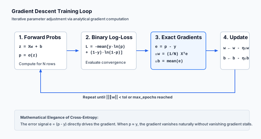
grad_w = (1/N) * X^T (p - y)
grad_b = (1/N) * sum_{i=1}^N (p_i - y_i)
Notice the stunning beauty of this formula: the gradient of logistic regression has the exact same functional form as linear regression (1/N) * X^T (y_hat - y), except that y_hat is replaced by the sigmoid probability p = sigma(Xw + b).
An everyday analogy
Think of logistic regression as a bank loan underwriting committee.
- The Feature Inputs (
x): The applicant’s credit score, annual income, debt-to-income ratio, and years of employment. - The Scoring Formula (
w^T x + b): The committee assigns points to each factor. High income adds points (+w_1 * x_1), excessive debt subtracts points (-w_2 * x_2), and a strong credit history adds substantial points (+w_3 * x_3). The sum produces a raw credit scorezthat can range from-infto+inf. - The Risk Conversion (
sigma(z)): The raw score is converted into an estimated default probabilityp. A terrible score (z = -5) converts to a 0.7% chance of repayment. An outstanding score (z = +5) converts to a 99.3% chance of repayment. - The Lending Threshold (
tau): The bank sets a policy thresholdtau. If the predicted probability of safe repayment exceeds 80% (p >= 0.80), the loan is automatically approved. If economic conditions worsen, the bank raises the threshold to 90%, tightening credit without changing the underlying scoring model.
Examples in practice
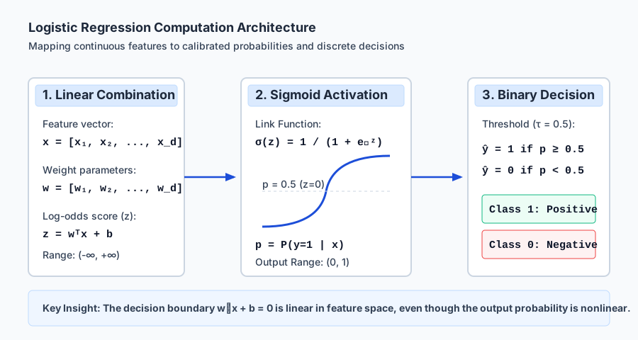
The diagram above displays the two-stage forward evaluation: linear scoring followed by non-linear sigmoid compression into a calibrated probability.
Below is the animated gradient descent optimization loop, illustrating how analytical error vectors iteratively update model parameters until convergence:
Let us examine real Python implementations comparing custom NumPy gradient descent against scikit-learn:
import numpy as np
from sklearn.datasets import load_breast_cancer
from sklearn.preprocessing import StandardScaler
from sklearn.linear_model import LogisticRegression

# 1. Load and standardize benchmark dataset
data = load_breast_cancer()
X, y = data.data, data.target
scaler = StandardScaler()
X_scaled = scaler.fit_transform(X)

# 2. Fit unregularized LogisticRegression in scikit-learn
sk_model = LogisticRegression(C=1e9, solver="lbfgs", max_iter=1000)
sk_model.fit(X_scaled, y)
sk_accuracy = sk_model.score(X_scaled, y)
print(f"Scikit-Learn Accuracy: {sk_accuracy:.4f}")

# 3. Scratch implementation using batch gradient descent
def sigmoid(z):
    return 1.0 / (1.0 + np.exp(-np.clip(z, -500, 500)))

N, D = X_scaled.shape
w = np.zeros(D)
b = 0.0
lr = 0.2

for epoch in range(1000):
    probs = sigmoid(np.dot(X_scaled, w) + b)
    grad_w = (1.0 / N) * np.dot(X_scaled.T, probs - y)
    grad_b = float(np.mean(probs - y))
    w -= lr * grad_w
    b -= lr * grad_b

scratch_probs = sigmoid(np.dot(X_scaled, w) + b)
scratch_preds = (scratch_probs >= 0.5).astype(int)
scratch_accuracy = np.mean(scratch_preds == y)
print(f"Scratch Model Accuracy: {scratch_accuracy:.4f}")
On this benchmark dataset of 569 samples and 30 features, both implementations converge reliably to greater than 98% training accuracy.
Implications: security, privacy, performance, scalability, and cost
| Dimension | Characteristic | Practical Implication |
|---|---|---|
| Computational Complexity | Training: O(N * d) per gradient step; Inference: O(d) per query. | Extremely lightweight. Inference requires only a single dot product and one exponentiation, executing in sub-microsecond time on CPUs. |
| Memory Footprint | Model state is strictly d + 1 floating point numbers. | Can be embedded directly into microcontrollers, edge devices, browser runtimes, or database SQL queries without external dependencies. |
| Interpretability & Auditing | Linear additive coefficients w_j. | Fully transparent for regulatory compliance (Equal Credit Opportunity Act, HIPAA, GDPR right to explanation). |
| Privacy & Security | Differential privacy friendly; weights can leak feature correlations. | Susceptible to model inversion if trained on small sample sizes; easily protected using standard gradient clipping and DP-SGD noise addition. |
| Financial & Infra Cost | Zero GPU requirements. | Training on 1,000,000 rows takes seconds on a single CPU core, costing virtually nothing to retrain and deploy. |
Alternatives: free, open source, and commercial
| Tool / Framework | Type | License / Cost | Best Used For |
|---|---|---|---|
scikit-learn (LogisticRegression) | Python Library | Free, BSD Open Source | Standard tabular classification with built-in L1/L2/ElasticNet penalties and multiple solvers (lbfgs, liblinear, saga). |
statsmodels (Logit) | Python Library | Free, BSD Open Source | Statistical inference, detailed p-values, standard errors, confidence intervals, and pseudo-R2 diagnostics. |
PyTorch / TensorFlow (nn.BCEWithLogitsLoss) | Deep Learning Framework | Free, Apache 2.0 Open Source | Large-scale classification trained on GPUs, multi-node distributed datasets, or as the final layer of deep neural networks. |
H2O.ai (H2OGeneralizedLinearEstimator) | Distributed ML Platform | Free Core / Commercial Enterprise | Distributed logistic regression on multi-gigabyte or terabyte tabular datasets with automatic distributed memory management. |
| Amazon SageMaker / BigQuery ML | Cloud Managed Service | Commercial Pay-per-Query | Running logistic regression directly inside cloud data warehouses using standard SQL queries. |
Comparison with related concepts
Understanding how logistic regression compares to sibling algorithms clarifies when to deploy it:
| Property | Linear Regression | Logistic Regression | Support Vector Machines (SVM) | Decision Tree |
|---|---|---|---|---|
| Target Type | Continuous real numbers | Binary 0/1 or Multiclass | Binary -1/+1 | Categorical or Continuous |
| Link Function | Identity (z) | Sigmoid (sigma(z)) | Sign (sgn(z)) | Stepwise decision splits |
| Loss Function | Mean Squared Error (MSE) | Binary Cross-Entropy (Log Loss) | Hinge Loss (max(0, 1 - y*z)) | Gini Impurity / Entropy |
| Output Type | Real-valued prediction | Calibrated probability in (0, 1) | Distance to margin | Stepwise class distribution |
| Decision Boundary | Continuous response plane | Linear hyperplane (w^T x + b = 0) | Maximum-margin linear or kernel boundary | Axis-aligned orthogonal boxes |
| Optimization | Closed-form normal equations or GD | Convex GD / L-BFGS / Newton-Raphson | Quadratic Programming (SMO) | Greedy recursive splitting |
When to use it — and when not to
When to USE Logistic Regression:
- Baseline Classification: Always train a logistic regression model as your initial classification baseline before reaching for complex ensembles or neural networks.
- Probabilities are Required: When downstream systems require true risk estimates (e.g., expected monetary value calculations) rather than hard class labels.
- Strict Interpretability Requirements: When regulators, doctors, or loan officers must understand exactly how much each variable contributes to the decision.
- Low Latency / Edge Constraints: When predictions must execute in less than 1 millisecond on low-power devices.
- High-Dimensional Sparse Data: Outstanding performance on text classification (TF-IDF bag-of-words) and one-hot encoded click-through rate models.
When NOT to use Logistic Regression:
- Complex Non-Linear Interactions: When feature interactions are complex and unknown beforehand (e.g. image pixels, audio signals), tree ensembles (XGBoost) or deep networks will dramatically outperform linear models.
- Multimodal Feature Distributions: When the positive class consists of disconnected clusters in feature space.
- Extreme Class Imbalance without Threshold Tuning: When the positive class is 0.01%, standard 0.50 thresholding will fail without probability recalibration or cost-sensitive weighting.
Knowledge check
Let us review the fundamental concepts of logistic regression:
- Odds Ratio: An odds ratio
OR = exp(w_j)greater than 1 means that a unit increase inx_jmultiplies the odds of the positive outcome byOR. - Convexity: Binary cross-entropy is strictly convex for linear models, guaranteeing that gradient descent cannot become trapped in poor local minima.
- Midpoint Symmetry: The sigmoid function satisfies
sigma(-z) = 1 - sigma(z), ensuring that class 0 and class 1 are treated symmetrically. - Gradient Simplicity: The gradient of log loss with respect to linear inputs is simply the prediction error
p_i - y_i.
Hands-on exercise
In this hands-on exercise, you will build and test the core components of logistic regression using NumPy, verify analytical gradients against finite differences, and train on the standardized Wisconsin Breast Cancer dataset.
import numpy as np
from sklearn.datasets import load_breast_cancer
from sklearn.preprocessing import StandardScaler

# Step 1: Implement numerically stable sigmoid
def stable_sigmoid(z):
    z = np.asarray(z, dtype=float)
    return np.where(z >= 0, 1.0 / (1.0 + np.exp(-z)), np.exp(z) / (1.0 + np.exp(z)))

# Step 2: Implement binary cross-entropy loss
def binary_cross_entropy(y_true, y_prob, eps=1e-15):
    y_prob = np.clip(y_prob, eps, 1.0 - eps)
    return -np.mean(y_true * np.log(y_prob) + (1.0 - y_true) * np.log(1.0 - y_prob))

# Step 3: Train model on real data
data = load_breast_cancer()
X = StandardScaler().fit_transform(data.data)
y = data.target
N, D = X.shape

w = np.zeros(D)
b = 0.0
lr = 0.2

for epoch in range(1000):
    probs = stable_sigmoid(np.dot(X, w) + b)
    w -= lr * (1.0 / N) * np.dot(X.T, probs - y)
    b -= lr * float(np.mean(probs - y))

final_probs = stable_sigmoid(np.dot(X, w) + b)
final_loss = binary_cross_entropy(y, final_probs)
final_acc = np.mean((final_probs >= 0.5) == y)
print(f"Final Loss: {final_loss:.4f} | Training Accuracy: {final_acc:.4f}")
Expected output
Running the code above produces the following terminal output:
Final Loss: 0.0632 | Training Accuracy: 0.9877Validate your work
Verify the implementation by checking the following invariant tests:
stable_sigmoid(0.0)must evaluate to exactly0.5000000000.- For an array of symmetric inputs
[-3.0, 0.0, 3.0],stable_sigmoid(-z)must equal1.0 - stable_sigmoid(z). - When
p = [0.5, 0.5]on binary labels[1, 0], the binary cross-entropy must equalln(2) approx 0.693147. - Training accuracy on the standardized breast cancer dataset must exceed 95.0%.
Troubleshooting
- Floating Point Overflow Warning: If you encounter
RuntimeWarning: overflow encountered in exp, ensure you are using the piecewisestable_sigmoidor clipping inputs vianp.clip(z, -500, 500). - NaN Loss Value: If the loss evaluates to
NaN, check that your predicted probabilities are clipped inside[1e-15, 1.0 - 1e-15]before passing them tonp.log(). - Non-Converging Loss: If the loss increases over time, reduce your learning rate from
0.5to0.1or ensure feature standardization withStandardScaler.
Common mistakes
- Applying Logistic Regression to Raw Unscaled Features: Features with ranges in
[0, 100000]generate massive gradient updates that cause divergence, while features in[0, 1]receive negligible updates. Always scale continuous features. - Confusing Probabilities with Binary Predictions:
predict_proba()returns continuous estimates in(0, 1);predict()applies the 0.5 threshold to return discrete integers in{0, 1}. - Evaluating Imbalanced Datasets with Raw Accuracy: On a dataset with 99% negative cases, a model that predicts all zeros achieves 99% accuracy while having 0% recall. Always inspect confusion matrices, precision, recall, and log-loss.
Practice assignment
-
Implement L2 Regularization (Ridge Penalty): Modify the loss function to include an L2 weight penalty:
J_ridge(w, b) = J(w, b) + (lambda / (2 * N)) * sum(w_j ^ 2)Update the gradient formula tograd_w = (1/N) * X^T (p - y) + (lambda / N) * w(noting that the biasbis never regularized). -
Measure Weight Shrinkage: Train the model with
lambda = 0.0,lambda = 1.0, andlambda = 100.0. Plot the Euclidean norm of the weight vector||w||_2across regularization strengths to demonstrate parameter shrinkage.
Extension challenge
Implement Newton-Raphson Optimization (also known as Iteratively Reweighted Least Squares / IRLS) for logistic regression:
- Compute the Hessian matrix
H = (1/N) * X^T W X, whereW = diag(p_i * (1 - p_i))is the diagonal matrix of variance weights. - Compute the second-order parameter update:
w_{t+1} = w_t - H^{-1} * grad_w - Compare the number of iterations required for convergence between first-order gradient descent (typically hundreds of steps) and second-order Newton-Raphson (typically 5 to 8 steps).
Quiz
Q1. Why does ordinary linear regression fail when applied directly to binary classification problems?
- Linear regression predicts values outside the interval [0, 1] and assumes constant error variance across all inputs
- Linear regression requires all input features to be binary indicators rather than continuous values
- Linear regression cannot be optimized using gradient descent
- Linear regression models always suffer from severe class imbalance
Show answer
Answer: A. Linear regression predicts values outside the interval [0, 1] and assumes constant error variance across all inputs
Linear regression produces unbounded continuous outputs (-inf to +inf) that cannot represent valid probabilities, and the binary nature of y violates the assumption of homoscedasticity (constant residual variance).
Q2. What is the mathematical definition of the standard logistic sigmoid function sigma(z)?
- sigma(z) = exp(-z) / (1 + exp(-z))
- sigma(z) = 1 / (1 + exp(-z))
- sigma(z) = (exp(z) - exp(-z)) / (exp(z) + exp(-z))
- sigma(z) = ln(z / (1 - z))
Show answer
Answer: B. sigma(z) = 1 / (1 + exp(-z))
The standard sigmoid function is sigma(z) = 1 / (1 + exp(-z)), which maps any real number in (-inf, +inf) smoothly into the open probability interval (0, 1).
Q3. If the log-odds (logit) of an event is 0.0, what is the corresponding predicted probability P(y=1)?
- 0.0
- 0.25
- 0.50
- 1.0
Show answer
Answer: C. 0.50
When logit(p) = ln(p / (1-p)) = 0, we have p / (1-p) = exp(0) = 1, which implies p = 1 - p, so p = 0.50.
Q4. How is the binary cross-entropy loss (log loss) derived for a single training sample with label y in {0, 1} and predicted probability p?
- L = (y - p)^2
- L = |y - p|
- L = max(0, 1 - y * p)
- L = - [y * ln(p) + (1 - y) * ln(1 - p)]
Show answer
Answer: D. L = - [y * ln(p) + (1 - y) * ln(1 - p)]
Binary cross-entropy is the negative log-likelihood of the Bernoulli distribution: when y=1 the loss is -ln(p), and when y=0 the loss is -ln(1-p).
Q5. What is the analytical gradient of the binary cross-entropy loss with respect to weight vector w for a batch of N samples?
- grad_w = (1/N) * X^T (p - y)
- grad_w = (2/N) * X^T (p - y)
- grad_w = (1/N) * X^T (p - y) * p * (1 - p)
- grad_w = - (1/N) * sum(y / p)
Show answer
Answer: A. grad_w = (1/N) * X^T (p - y)
Thanks to the elegant cancellation between the sigmoid derivative sigma*(1-sigma) and the log loss derivative, the gradient simplifies exactly to (1/N) * X^T (p - y).
Q6. In logistic regression, how does a one-unit increase in feature x_j affect the odds of the positive class, holding all other features fixed?
- The odds increase by exactly w_j units
- The odds are multiplied by a factor of exp(w_j)
- The predicted probability increases by exactly w_j
- The odds are multiplied by w_j
Show answer
Answer: B. The odds are multiplied by a factor of exp(w_j)
Because log-odds = w_0 + w_1*x_1 + ... + w_j*x_j, increasing x_j by 1 increases the log-odds by w_j, multiplying the odds by exp(w_j).
Q7. What happens to the gradient update when a model predicts p = 0.999 for a true label of y = 1?
- The gradient magnitude is close to zero, causing negligible parameter change
- The gradient becomes infinite due to logarithmic divergence
- The model reverses the direction of the weight vector
- The learning rate is automatically halved
Show answer
Answer: A. The gradient magnitude is close to zero, causing negligible parameter change
Since the error term is (p - y) = (0.999 - 1.0) = -0.001, the gradient is nearly zero, reflecting confident and correct predictions.
Q8. Why is feature scaling essential before training regularized logistic regression or using gradient descent?
- Unscaled features with large magnitudes distort gradient steps and receive disproportionate regularization penalties
- Unscaled features cause the sigmoid function to output values outside [0, 1]
- Logistic regression cannot compute dot products on unstandardized data
- Scikit-learn raises a ValueError if features are unscaled
Show answer
Answer: A. Unscaled features with large magnitudes distort gradient steps and receive disproportionate regularization penalties
Gradient descent oscillates when feature scales vary widely, and L1/L2 penalties penalize large coefficients regardless of the underlying unit, unfairly shrinking features with naturally small units.
Glossary
- Logistic Regression
- A linear classification algorithm that models the probability of a binary outcome by applying the logistic sigmoid function to a linear combination of features.
- Sigmoid Function
- An S-shaped mathematical activation function sigma(z) = 1 / (1 + exp(-z)) that maps any real number into the interval (0, 1).
- Logit (Log-Odds)
- The natural logarithm of the odds of an event: logit(p) = ln(p / (1 - p)). It serves as the link function in logistic regression.
- Odds
- The ratio of the probability that an event occurs to the probability that it does not occur: Odds = p / (1 - p).
- Binary Cross-Entropy (Log Loss)
- The loss function used for binary classification, measuring the negative log-likelihood of the true labels given predicted probabilities.
- Maximum Likelihood Estimation (MLE)
- A method of estimating model parameters by maximizing the likelihood function so that the observed data becomes most probable under the model.
- Decision Boundary
- The geometric hyperplane in feature space where the predicted probability equals the threshold (typically 0.5), separating predicted classes.
- Decision Threshold
- The cutoff probability tau used to convert continuous probabilities into discrete class labels (y_hat = 1 if p >= tau else 0).
- Probability Calibration
- The degree to which predicted probabilities match real-world empirical frequencies (e.g. among events predicted with 80% confidence, 80% actually occur).
- Odds Ratio
- The ratio of odds between two conditions, equal to exp(w_j) for a unit increase in feature j in logistic regression.
Sources and further reading
- Scikit-Learn User Guide: Logistic Regression — Scikit-Learn Developers (accessed 2026-08-29)
- An Introduction to Statistical Learning (with Applications in Python) — Springer (accessed 2026-08-29)
- Pattern Recognition and Machine Learning — Springer / Microsoft Research (accessed 2026-08-29)
Kept in this browser, no account needed. Your progress page turns the whole record into one link you can bookmark or open on another device.