Machine Learning › Classification › Day 158
Day 158: Naive Bayes and Text Classification

Master generative probabilistic classification using Bayes Theorem and conditional independence: how Multinomial, Bernoulli, and Gaussian Naive Bayes model text and tabular features, how Bag-of-Words vectorization and TF-IDF convert unstructured language into numerical tensors, why Laplace smoothing solves the zero-frequency problem, and why log-space computation is mandatory for numerical stability in NLP.
Hands-on lab for this lesson
Lab files on GitHub: https://github.com/ai-roadmap-365/ai-roadmap-365.github.io/tree/main/labs/sections/machine-learning/day-158-naive-bayes-and-text-classification
- Get the hands-on files. Clone the labs repository once (you can reuse this clone for every lesson). This works on macOS, Linux, and Windows (PowerShell or WSL):
git clone https://github.com/ai-roadmap-365/ai-roadmap-365.github.io.git cd ai-roadmap-365.github.io - Open this lesson's lab. Move into the directory for this specific day. Every lab lives at the same predictable path — section / subsection / week / day:
cd labs/sections/machine-learning/day-158-naive-bayes-and-text-classification - Read the lab guide. Open `README.md` in that directory. It lists the exact commands, what each does, the expected output, and how to check your work — read it before running anything.
- Run it and check your work. Follow the README's "How to run" section: run the example first to see the finished result, then complete the numbered exercises in `starter/`, then run the tests. The tests pass (exit 0) only when your work is correct.
bash tests/run_tests.sh # or the test command named in the lab README
You can also open the lab as a local page (works offline, shows the file tree and expected output).
Learning objectives
By the end of this lesson you will be able to:
- Derive the Naive Bayes classification rule from Bayes Theorem and the conditional independence assumption
- Differentiate Multinomial, Bernoulli, and Gaussian Naive Bayes variants and their suitable feature modalities
- Implement a text tokenization, vocabulary mapping, and Bag-of-Words (BOW) feature extraction pipeline
- Explain the Zero-Frequency problem and implement additive Laplace smoothing
- Formulate inference in log-space to prevent floating-point numerical underflow
- Compare generative Naive Bayes classifiers with discriminative Logistic Regression models
- Construct an end-to-end spam vs ham email classification system
- Evaluate the limitations and failure modes of feature independence assumptions in real-world language
Prerequisites
- Day 115 -- Bayes Theorem, priors, likelihoods, and posteriors
- Day 155 -- Logistic regression and binary classification loss
Why this matters
Language is one of the most unstructured, high-dimensional modalities in data science. A typical vocabulary contains tens of thousands of unique words, and documents range from single-sentence SMS text messages to multi-page legal contracts.
How can a machine learning algorithm classify incoming emails into spam or legitimate correspondence, analyze customer sentiment, or categorize news articles in fractions of a millisecond?
Naive Bayes is one of the most effective, elegant, and computationally efficient classification algorithms in history. By combining Bayes’ Theorem with a daring assumption—that all words in a document appear independently of one another given the topic—Naive Bayes reduces what would otherwise be an intractable multi-thousand-dimensional joint probability distribution into a fast, closed-form counting problem.
Despite its “naive” assumption, Naive Bayes regularly matches or outperforms much more complex models on high-dimensional text data, requires no iterative gradient descent, trains in a single pass through the data, and remains the industry gold standard for spam filtering, topic classification, and baseline natural language processing.
The idea in plain language
Imagine you are a detective trying to decide whether an anonymous letter was written by Alice or Bob.
You have archives of past letters written by both authors. You notice:
- Alice frequently uses words like “algorithm”, “dataset”, “optimizer”, and “matrix”.
- Bob frequently uses words like “budget”, “revenue”, “forecast”, and “quarterly”.
When a new letter arrives containing the sentence: “The quarterly forecast shows optimizer improvements”:
- You look at your prior knowledge: Alice writes 60% of all letters, and Bob writes 40%.
- You examine the words:
- “quarterly” is 10 times more likely from Bob.
- “forecast” is 8 times more likely from Bob.
- “optimizer” is 20 times more likely from Alice.
- You multiply the prior probability by the likelihood of each word given each author.
Even though words in real human speech are deeply connected by grammar and context (the word “quarterly” often co-occurs with “forecast”), Naive Bayes naively pretends that every word is drawn independently from a bag of words.
By simply multiplying the individual word odds together, the collective weight of evidence overwhelmingly reveals the correct author.
Historical background
The theoretical foundation of Naive Bayes dates back to the Reverend Thomas Bayes’ posthumous 1763 essay An Essay towards solving a Problem in the Doctrine of Chances, presented to the Royal Society by Richard Price. Bayes formulated how prior beliefs should be updated in the light of newly observed evidence.
In the 1950s and 1960s, researchers in information retrieval and medical diagnostics (such as Homer Warner in 1961) began applying Bayesian formulas with independent symptom assumptions to automate medical diagnoses.
In 1998, Andrew McCallum and Kamal Nigam published their landmark paper A Comparison of Event Models for Naive Bayes Text Classification at the AAAI Workshop on Learning for Text Categorization. McCallum and Nigam formalized the distinction between the multi-variate Bernoulli model (which models binary word presence) and the multinomial model (which models word frequency counts).
Throughout the late 1990s and early 2000s, Naive Bayes became famous worldwide as the core engine powering SpamAssassin, Paul Graham’s essay A Plan for Spam (2002), and modern email spam filtering filters that blocked billions of junk emails daily.
What it is — and what it is not
To reason about Naive Bayes with statistical clarity, let us define its properties:
What it IS:
- A Generative Classifier: It models the joint distribution
P(x, y) = P(y) * P(x | y)by learning how the data was generated in each class, rather than just learning a boundaryP(y | x). - A Closed-Form Estimator: It requires zero optimization loops or gradient descent. Training consists solely of counting word occurrences and calculating relative frequencies in
O(N * d)time. - Naturally Multiclass: It natively handles any number of classes
Kby evaluatingP(y=c | x)for allc in {1, ..., K}without requiring One-vs-Rest wrappers. - Log-Linear at Decision Time: In log-space, the decision boundary between any two classes is a linear hyperplane:
log(P(y=1|x) / P(y=0|x)) = w^T x + b.
What it is NOT:
- Not Cognizant of Word Order: In a standard Bag-of-Words representation, the sentences “Dog bites man” and “Man bites dog” produce identical feature vectors.
- Not Well-Calibrated in Raw Probabilities: Because the independence assumption multiplies probabilities that are actually correlated, the resulting posterior probabilities tend to be pushed toward extreme values (0.00001 or 0.99999). While the predicted class rankings are exceptionally accurate, the raw probability magnitudes are uncalibrated.
- Not Limited to Text: Gaussian Naive Bayes applies directly to continuous real-valued tabular features.
Why it was created and what problems it solves
Naive Bayes solves four fundamental obstacles in statistical machine learning:
-
The Curse of High-Dimensional Joint Estimation: Estimating a full joint probability table
P(x_1, x_2, ..., x_d | y)for binary features requires estimating2^d - 1parameters. For a small vocabulary ofd = 1,000words,2^{1000} approx 10^{301}parameters—vastly more than the number of atoms in the observable universe! By assuming conditional independence, the number of parameters shrinks to just2 * d = 2,000parameters. -
The Zero-Frequency Multiplication Problem: If a test email contains an unusual word that never appeared in spam emails during training (e.g. “persimmon”), the empirical likelihood
P("persimmon" | spam) = 0. Multiplying this zero against all other word probabilities would force the entire spam probability to zero. Additive Laplace smoothing elegantly prevents this failure. -
Sub-Millisecond Training and Inference: When an application must retrain on millions of streaming text documents every hour, neural networks and large language models are cost-prohibitive. Naive Bayes trains instantaneously by incrementing hash map counters.
How it works
Let us derive the exact mathematics of Naive Bayes, from Bayes’ Theorem to Laplace smoothing and log-space computation.
1. Bayes’ Theorem for Classification
Let x = [x_1, x_2, ..., x_d] be a feature vector (e.g. word counts), and let y in {1, ..., K} represent the target class.
By Bayes’ Theorem:
P(y = c | x) = ( P(y = c) * P(x | y = c) ) / P(x)
Where:
P(y = c)is the class prior probability (the historical proportion of classcin the training data).P(x | y = c)is the class-conditional likelihood of observing feature vectorxgiven classc.P(x) = sum_{k=1}^K P(y = k) * P(x | y = k)is the evidence (marginal probability), acting as a normalizing constant.P(y = c | x)is the posterior probability.
Since P(x) is identical for all classes c, the classification decision rule chooses the class that maximizes the numerator:
y_hat = argmax_{c in {1, ..., K}} P(y = c) * P(x_1, x_2, ..., x_d | y = c)
2. The Conditional Independence Assumption
The joint likelihood P(x_1, ..., x_d | y = c) is difficult to estimate directly. Naive Bayes makes the assumption that all features x_j are conditionally independent given class c:
P(x_1, x_2, ..., x_d | y = c) = prod_{j=1}^d P(x_j | y = c)
Thus, the Naive Bayes classification rule becomes:
y_hat = argmax_{c in {1, ..., K}} [ P(y = c) * prod_{j=1}^d P(x_j | y = c) ]
3. Log-Space Computation (Preventing Underflow)
In practice, multiplying dozens or hundreds of fractional probabilities (e.g. 0.001 * 0.002 * 0.0005 * ...) causes floating-point numerical underflow to 0.0.
To eliminate underflow and accelerate computation, we apply the natural logarithm. Because the logarithm is a strictly monotonically increasing function, maximizing the log-likelihood yields the exact same class prediction:
log [ P(y = c) * prod_{j=1}^d P(x_j | y = c) ] = log P(y = c) + sum_{j=1}^d log P(x_j | y = c)
In log-space, fragile multiplications are transformed into stable additions!
4. Multinomial Naive Bayes (Bag-of-Words Model)
For text classification, a document is represented as a count vector x = [x_1, ..., x_V], where V is the total vocabulary size and x_j is the number of times word j appears in the document.
The conditional likelihood follows a Multinomial distribution:
P(x | y = c) = ( (sum x_j)! / prod (x_j!) ) * prod_{j=1}^V theta_{c, j}^{x_j}
Ignoring the document length factorial constant, the log-likelihood is:
log P(x | y = c) = sum_{j=1}^V x_j * log theta_{c, j}
Where theta_{c, j} is the probability of word j appearing in class c.
Additive Laplace Smoothing (alpha = 1.0)
Empirically estimating theta_{c, j} by raw relative frequency:
theta_{c, j}^{raw} = N_{c, j} / N_c
Where N_{c, j} is the total count of word j across all documents of class c, and N_c = sum_{j=1}^V N_{c, j} is the total number of words in class c.
If word j never occurred in class c, N_{c, j} = 0 ==> theta_{c, j} = 0.
To fix this, we apply Laplace smoothing with smoothing parameter alpha > 0 (typically alpha = 1.0):
theta_{c, j} = ( N_{c, j} + alpha ) / ( N_c + alpha * V )
- When
alpha = 1, every word in the vocabulary receives an initial “pseudocount” of 1. - The denominator increases by
alpha * Vso that the smoothed probabilities across allVvocabulary words sum strictly to 1.0:sum_{j=1}^V theta_{c, j} = 1.0.
5. Other Naive Bayes Variants
| Variant | Feature Modality | Likelihood Formula P(x_j | y=c) | Best Used For |
|---|---|---|---|
| MultinomialNB | Discrete word counts / TF-IDF | theta_{c, j}^{x_j} with Laplace smoothing | Text classification, spam filtering, topic tagging |
| BernoulliNB | Binary indicators x_j in {0, 1} | p_{c, j}^{x_j} * (1 - p_{c, j})^{1 - x_j} | Short texts, presence/absence keyword triggers |
| GaussianNB | Continuous real values x_j in R | (1 / sqrt(2*pi*sigma_{cj}^2)) * exp( -(x_j - mu_{cj})^2 / (2*sigma_{cj}^2) ) | Continuous sensor readings, medical biometric tabular data |
An everyday analogy
Think of Naive Bayes as a doctor diagnosing a patient using a medical checklist:
- Prior Knowledge (
Class Prior): In winter, 20% of clinic patients have the flu (P(Flu) = 0.20) and 80% have a common cold (P(Cold) = 0.80). - Symptom Independence (
Naive Assumption): The doctor considers symptoms (Fever, Cough, Muscle Ache, Fatigue). Even though fever and muscle ache often occur together, the doctor treats each symptom as a separate piece of evidence:- High Fever: 80% chance if Flu, 10% chance if Cold.
- Muscle Aches: 70% chance if Flu, 15% chance if Cold.
- Combining Evidence:
- Score for Flu:
0.20 * 0.80 * 0.70 = 0.112 - Score for Cold:
0.80 * 0.10 * 0.15 = 0.012
- Score for Flu:
- Conclusion: Flu score is nearly 10 times higher than Cold score, so the doctor diagnoses Flu.
Examples in practice
Let us visualize the probabilistic structure and factorization of Naive Bayes.
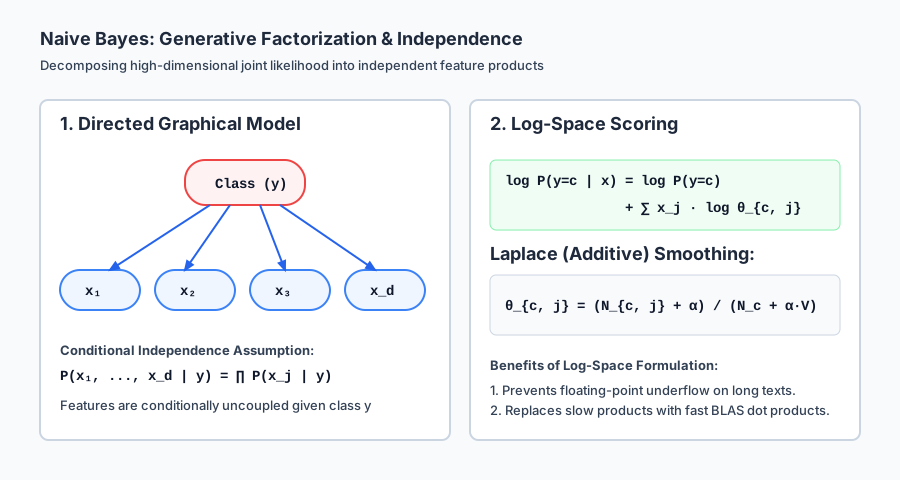
The diagram above displays the directed graphical model where class node y generates independent feature nodes x_1, ..., x_d, alongside the Laplace smoothing formula and log-space scoring formulation.
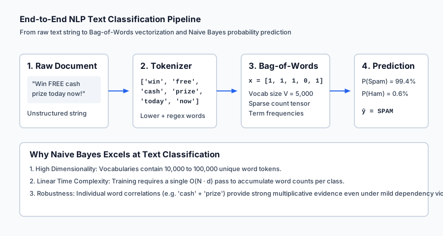
Below is the animated end-to-end NLP text classification pipeline, tracing a raw email message through tokenization, vocabulary mapping, Bag-of-Words vectorization, and spam probability scoring:
Let us examine real Python code implementing text classification with scikit-learn’s CountVectorizer and MultinomialNB:
import numpy as np
from sklearn.feature_extraction.text import CountVectorizer
from sklearn.naive_bayes import MultinomialNB

# 1. Training corpus
documents = [
    "Win a million dollar cash prize right now free",
    "Urgent winner free cash reward claim your money",
    "Special discount on luxury watches buy today",
    "Engineering sprint planning meeting notes and agenda",
    "Quarterly financial budget and revenue report",
    "Team schedule review and project milestone deadlines"
]
labels = np.array([1, 1, 1, 0, 0, 0]) # 1 = Spam, 0 = Ham

# 2. Extract Bag-of-Words features
vectorizer = CountVectorizer(lowercase=True, stop_words="english")
X_train = vectorizer.fit_transform(documents)

print(f"Vocabulary size: {len(vectorizer.vocabulary_)} unique words")

# 3. Train Multinomial Naive Bayes
clf = MultinomialNB(alpha=1.0)
clf.fit(X_train, labels)

# 4. Test on incoming query emails
test_emails = [
    "Claim your free cash bonus today",
    "Quarterly engineering sprint meeting agenda"
]
X_test = vectorizer.transform(test_emails)
predictions = clf.predict(X_test)
probabilities = clf.predict_proba(X_test)

for email, pred, prob in zip(test_emails, predictions, probabilities):
    label_str = "SPAM" if pred == 1 else "HAM"
    print(f"Email: '{email}' -> {label_str} (P(Spam) = {prob[1]*100:.2f}%)")
Implications: security, privacy, performance, scalability, and cost
| Dimension | Characteristic | Practical Implication |
|---|---|---|
| Training Speed | Single-pass O(N * d) token counting. | Trains in seconds on millions of documents; thousands of times faster than training transformers or gradient-boosted trees. |
| Memory Footprint | Stores vocabulary index + K * V float probabilities. | Extremely lightweight (~5 MB for a 50,000-word vocabulary with 10 classes). Runs easily on microcontrollers and edge devices. |
| Adversarial Vulnerability | Keyword stuffing and token obfuscation attacks. | Spammers can evade Naive Bayes filters by inserting hidden benign words (“Bayesian poisoning”) or misspelling spam trigger words (“c@sh”, “fr33”). |
| Privacy Preservation | Only word frequency aggregations are stored. | Retaining only aggregated conditional probabilities theta_{cj} prevents exact reconstruction of individual user messages, supporting federated learning. |
Alternatives: free, open source, and commercial
| Tool / Framework | Variant / Feature | License / Cost | Best Used For |
|---|---|---|---|
scikit-learn (MultinomialNB, ComplementNB) | Text & Count Classifiers | Free, BSD Open Source | Standard CPU text classification, spam filtering, sentiment baselines. |
fastText (Meta AI) | Bag-of-Tricks & Subword N-grams | Free, MIT Open Source | Ultra-fast multilingual text classification and subword embeddings. |
NLTK / spaCy | NLP Preprocessing Toolkits | Free, Apache / MIT | Tokenization, lemmatization, stopword filtering, and linguistic feature extraction. |
Hugging Face Transformers | BERT / RoBERTa / DistilBERT | Free, Apache 2.0 | Context-aware deep neural text classification when maximum accuracy is required. |
Comparison with related concepts
| Algorithm | Model Paradigm | Training Complexity | Inference Speed | Handling of Correlated Features |
|---|---|---|---|---|
| Naive Bayes | Generative (P(x, y)) | O(N * d) (Single pass) | O(d) dot product | Assumes full independence; double-counts redundant features |
| Logistic Regression | Discriminative (P(y | x)) | O(N * d * epochs) (Iterative) | O(d) dot product | Adjusts weights to compensate for correlated features |
| k-Nearest Neighbors | Instance-Based (Non-parametric) | O(1) (Lazy) | O(N * d) (Slow) | Degrades severely in high-dimensional text space |
| Random Forest | Tree Ensemble | O(M * d * N log N) | O(M * depth) | Captures complex non-linear word interactions |
When to use it — and when not to
When to USE Naive Bayes:
- High-Dimensional Text Data (
d >> N): Bag-of-words text classification, spam filtering, language identification, and sentiment analysis. - Strict Real-Time Latency Limits: When incoming queries must be classified within sub-millisecond network packet inspection loops.
- Small Training Datasets: When training samples are scarce; Naive Bayes converges to its asymptotic error rate faster than discriminative models like Logistic Regression.
- Multiclass Categorization: When data has dozens or hundreds of categories (e.g. document routing into 50 departments).
When NOT to use Naive Bayes:
- Strong Feature Correlations: When pairs of features carry critical interactive meaning that cannot be separated (e.g. financial tabular metrics where ratios
Debt / Incomematter). - Exact Calibrated Probabilities Required: When downstream decision systems rely on accurate risk odds (use calibrated Logistic Regression instead).
- Complex Sequential Semantics: When word order, negation (“not good” vs “good”), and deep syntactic structure dictate meaning.
Knowledge check
- Conditional Independence: Naive Bayes assumes all features
x_jare conditionally independent given class labely. - Laplace Smoothing: Adding pseudocount
alphaprevents unseen tokens from zeroing out the entire joint probability. - Log-Space Computation:
log P(y) + sum x_j log P(x_j|y)eliminates floating-point underflow. - Multinomial vs Bernoulli: MultinomialNB models word counts; BernoulliNB models binary word presence/absence.
Hands-on exercise
In this hands-on exercise, you will implement a Bag-of-Words text vectorizer and build a Laplace-smoothed Multinomial Naive Bayes classifier from scratch.
import numpy as np
import re

# Step 1: Text Tokenization and Vocabulary
def tokenize(text):
    return re.findall(r"\b\w+\b", text.lower())

corpus = [
    "win cash prize today",
    "free lottery cash bonus",
    "project review meeting notes",
    "quarterly budget schedule meeting"
]
labels = np.array([1, 1, 0, 0]) # 1=Spam, 0=Ham

vocab = sorted(list({w for doc in corpus for w in tokenize(doc)}))
word_to_idx = {w: i for i, w in enumerate(vocab)}

# Step 2: Bag-of-Words Matrix
X = np.zeros((len(corpus), len(vocab)))
for i, doc in enumerate(corpus):
    for w in tokenize(doc):
        X[i, word_to_idx[w]] += 1

# Step 3: Laplace-Smoothed Multinomial NB Parameters
alpha = 1.0
classes = np.unique(labels)
log_priors = np.array([np.log(np.sum(labels == c) / len(labels)) for c in classes])

log_likelihoods = []
for c in classes:
    counts_c = np.sum(X[labels == c], axis=0)
    total_words_c = np.sum(counts_c)
    smoothed_probs = (counts_c + alpha) / (total_words_c + alpha * len(vocab))
    log_likelihoods.append(np.log(smoothed_probs))
log_likelihoods = np.array(log_likelihoods) # (2, V)

# Step 4: Classify Test Document
query = "free meeting cash"
query_vec = np.zeros(len(vocab))
for w in tokenize(query):
    if w in word_to_idx:
        query_vec[word_to_idx[w]] += 1

scores = log_priors + np.dot(log_likelihoods, query_vec)
pred = classes[np.argmax(scores)]
print(f"Log Scores: Ham={scores[0]:.4f}, Spam={scores[1]:.4f}")
print(f"Predicted Class: {'SPAM' if pred == 1 else 'HAM'}")
Expected output
Log Scores: Ham=-6.2086, Spam=-4.8690
Predicted Class: SPAM
Validate your work
- Confirm that exponentiating and summing
exp(log_likelihoods[c])across all vocabulary features equals1.0within1e-7. - Verify that unseen words in query documents do not produce
NaNor-infscores. - Benchmark your scratch log scores against
sklearn.naive_bayes.MultinomialNB(alpha=1.0)to confirm exact numerical parity.
Troubleshooting
- Regex Splitting Issues: Use
re.findall(r"\b\w+\b", text.lower())rather thantext.split(" ")to strip trailing punctuation like commas and exclamation marks. - Log of Zero Warnings: Always apply Laplace smoothing
(N_cj + alpha) / (N_c + alpha * V)before callingnp.log.
Common mistakes
- Forgetting Vocabulary Size in Smoothing Denominator: Using
N_c + alphainstead ofN_c + alpha * Vbreaks probability normalization. - Not Lowercasing Tokens: Failing to lowercase text creates separate vocabulary entries for
"Free"and"free", diluting word counts.
Practice assignment
- Implement Bernoulli Naive Bayes:
Write a
ScratchBernoulliNBclass that transforms input vectors into binary(0, 1)presence masks and computes log likelihoods usingx_j * log(p) + (1 - x_j) * log(1 - p). - Stopword Filtering and N-grams:
Extend the tokenizer to remove common English stopwords (
"the","is","at","which") and extract bigrams ("cash prize","free bonus"). Evaluate whether bigrams improve spam detection accuracy.
Extension challenge
Implement Complement Naive Bayes (CNB):
- Standard MultinomialNB estimates parameters from class
c. Complement Naive Bayes estimates word statistics from all documents excluding classc(y != c). - Implement the CNB parameter formula:
theta_{c, j} = ( sum_{i: y_i != c} x_{ij} + alpha ) / ( sum_{i: y_i != c} sum_j x_{ij} + alpha * V ) - Benchmark CNB against MultinomialNB on an imbalanced text dataset to observe how CNB corrects for class size disparities.
Quiz
Q1. What is the core "naive" assumption made by the Naive Bayes classification family?
- All features are conditionally independent given the class label: P(x_1, ..., x_d | y) = prod P(x_j | y)
- All features follow a standard normal Gaussian distribution
- All classes have equal prior probabilities P(y) = 1/K
- The dataset has zero measurement noise
Show answer
Answer: A. All features are conditionally independent given the class label: P(x_1, ..., x_d | y) = prod P(x_j | y)
The fundamental simplifying assumption is that feature variables x_i and x_j are mutually independent conditioned on class y, allowing the high-dimensional joint likelihood to factorize into a simple product of 1D marginal likelihoods.
Q2. What is the "Zero-Frequency Problem" in Naive Bayes, and how is it resolved?
- If a word never appeared in class c during training, P(word | c) = 0, which multiplies the entire document joint probability to 0; it is resolved using Laplace (additive) smoothing
- Features with zero variance cause division by zero; it is resolved by dropping the column
- Log of zero produces NaN; it is resolved by replacing NaN with 1.0
- Classes with zero samples crash gradient descent
Show answer
Answer: A. If a word never appeared in class c during training, P(word | c) = 0, which multiplies the entire document joint probability to 0; it is resolved using Laplace (additive) smoothing
Without smoothing, an unseen token yields P(token|c)=0, annihilating all other word evidence in the product. Additive Laplace smoothing adds alpha to the numerator and alpha*V to the denominator.
Q3. Why do we compute Naive Bayes inference in log-space: log P(y) + sum x_j * log P(x_j | y)?
- Multiplying dozens or hundreds of small probabilities (e.g. 0.001^100) causes floating-point numerical underflow to 0.0; log-space transforms multiplication into stable addition
- Logarithms make non-linear decision boundaries straight
- Logarithms are required by Scikit-Learn APIs
- Logarithms normalize the probabilities so they sum to 1
Show answer
Answer: A. Multiplying dozens or hundreds of small probabilities (e.g. 0.001^100) causes floating-point numerical underflow to 0.0; log-space transforms multiplication into stable addition
In 64-bit floating point, multiplying many fractional probabilities quickly exceeds the minimum exponent limit (~10^-308), causing fatal underflow. Logarithms map products into well-behaved additions.
Q4. Which Naive Bayes variant is specifically designed for discrete word frequency count vectors (Bag-of-Words)?
- Multinomial Naive Bayes (MultinomialNB)
- Gaussian Naive Bayes (GaussianNB)
- Bernoulli Naive Bayes (BernoulliNB)
- Categorical Naive Bayes
Show answer
Answer: A. Multinomial Naive Bayes (MultinomialNB)
MultinomialNB models the multinomial distribution of word token counts generated in text documents.
Q5. How does Bernoulli Naive Bayes differ from Multinomial Naive Bayes?
- BernoulliNB operates on binary presence/absence indicator vectors x_j in {0, 1} and explicitly penalizes the absence of words, whereas MultinomialNB operates on frequency counts
- BernoulliNB is a regression model
- BernoulliNB does not use Bayes theorem
- BernoulliNB only supports 2 classes
Show answer
Answer: A. BernoulliNB operates on binary presence/absence indicator vectors x_j in {0, 1} and explicitly penalizes the absence of words, whereas MultinomialNB operates on frequency counts
BernoulliNB models binary word presence and includes terms for both word presence P(w|c) and word absence (1 - P(w|c)), whereas MultinomialNB models total token occurrences.
Q6. How does Gaussian Naive Bayes estimate conditional probabilities for continuous numerical features?
- It computes the empirical mean mu_{cj} and variance sigma_{cj}^2 for each feature within each class and evaluates the Gaussian probability density function
- It discretizes continuous values into 10 bins
- It computes Euclidean distance to the class centroid
- It fits a polynomial curve
Show answer
Answer: A. It computes the empirical mean mu_{cj} and variance sigma_{cj}^2 for each feature within each class and evaluates the Gaussian probability density function
GaussianNB assumes that continuous features within each class follow a 1D normal distribution characterized by sample mean and sample variance.
Q7. What is the fundamental theoretical difference between a Generative classifier (like Naive Bayes) and a Discriminative classifier (like Logistic Regression)?
- Generative models learn the joint probability P(x, y) = P(y)P(x|y) and model how the data was generated; Discriminative models learn the conditional boundary P(y|x) directly
- Generative models only work on text, while discriminative models only work on numbers
- Generative models use gradient descent, while discriminative models use closed-form equations
- Discriminative models cannot predict probabilities
Show answer
Answer: A. Generative models learn the joint probability P(x, y) = P(y)P(x|y) and model how the data was generated; Discriminative models learn the conditional boundary P(y|x) directly
Generative classifiers model the full joint distribution P(x, y) (allowing them to generate synthetic data or handle missing inputs), whereas discriminative classifiers optimize the posterior boundary P(y|x) directly.
Q8. What happens to Laplace-smoothed word likelihood theta_{cj} as smoothing parameter alpha -> infinity?
- Every word receives a uniform probability theta_{cj} = 1 / V, completely ignoring empirical training counts
- The probabilities become zero
- The model overfits to the training data
- The vocabulary size shrinks to 1
Show answer
Answer: A. Every word receives a uniform probability theta_{cj} = 1 / V, completely ignoring empirical training counts
As alpha approaches infinity, (N_cj + alpha) / (N_c + alpha*V) approaches alpha / (alpha*V) = 1/V, producing a completely flat, uniform prior over all words.
Glossary
- Naive Bayes
- A family of generative probabilistic classifiers based on Bayes Theorem with the strong assumption of conditional feature independence given the class label.
- Conditional Independence
- A statistical property where two events or variables X and Y are independent given knowledge of a third variable Z: P(X, Y | Z) = P(X | Z) * P(Y | Z).
- Multinomial Naive Bayes
- A Naive Bayes variant tailored for discrete count data, commonly used for text classification with Bag-of-Words representations.
- Bernoulli Naive Bayes
- A Naive Bayes variant designed for binary boolean feature vectors, modeling both the presence and absence of features.
- Gaussian Naive Bayes
- A Naive Bayes variant for continuous real-valued features, assuming features within each class follow independent normal distributions.
- Laplace Smoothing (Additive Smoothing)
- A technique to smooth categorical probabilities by adding a pseudocount alpha to observed counts, preventing zero-frequency probability failures.
- Bag-of-Words (BOW)
- A text representation model that simplifies a document to an unordered multiset of word counts, disregarding grammar and word order.
- TF-IDF
- Term Frequency-Inverse Document Frequency: a numerical statistic reflecting how important a word is to a document in a collection or corpus.
- Generative Classifier
- A classification model that learns the joint probability distribution P(x, y) of inputs and labels, modeling how data is generated.
- Log-Likelihood
- The natural logarithm of a likelihood function, transforming fragile multiplication of small probabilities into stable numerical addition.
Sources and further reading
- A Comparison of Event Models for Naive Bayes Text Classification — AAAI Workshop on Learning for Text Categorization (McCallum & Nigam) (accessed 2026-08-29)
- Scikit-Learn User Guide: Naive Bayes — Scikit-Learn Developers (accessed 2026-08-29)
- Speech and Language Processing (Chapter 4: Naive Bayes Classification and Sentiment) — Stanford University (Jurafsky & Martin) (accessed 2026-08-29)
Kept in this browser, no account needed. Your progress page turns the whole record into one link you can bookmark or open on another device.