Machine Learning › Classification › Day 159
Day 159: Precision, Recall, ROC, and Choosing Thresholds

Master the rigorous evaluation of classification models: why accuracy is a dangerous illusion on imbalanced data, how the confusion matrix defines Precision, Recall, Specificity, F-beta, and Matthews Correlation Coefficient (MCC), how threshold sweeping generates Receiver Operating Characteristic (ROC) and Precision-Recall (PR) curves, how to calculate AUC metrics, and how to select optimal decision thresholds based on real-world cost trade-offs.
Hands-on lab for this lesson
Lab files on GitHub: https://github.com/ai-roadmap-365/ai-roadmap-365.github.io/tree/main/labs/sections/machine-learning/day-159-precision-recall-roc-and-choosing-thresholds
- Get the hands-on files. Clone the labs repository once (you can reuse this clone for every lesson). This works on macOS, Linux, and Windows (PowerShell or WSL):
git clone https://github.com/ai-roadmap-365/ai-roadmap-365.github.io.git cd ai-roadmap-365.github.io - Open this lesson's lab. Move into the directory for this specific day. Every lab lives at the same predictable path — section / subsection / week / day:
cd labs/sections/machine-learning/day-159-precision-recall-roc-and-choosing-thresholds - Read the lab guide. Open `README.md` in that directory. It lists the exact commands, what each does, the expected output, and how to check your work — read it before running anything.
- Run it and check your work. Follow the README's "How to run" section: run the example first to see the finished result, then complete the numbered exercises in `starter/`, then run the tests. The tests pass (exit 0) only when your work is correct.
bash tests/run_tests.sh # or the test command named in the lab README
You can also open the lab as a local page (works offline, shows the file tree and expected output).
Learning objectives
By the end of this lesson you will be able to:
- Construct and interpret the 2x2 confusion matrix (TN, FP, FN, TP)
- Derive Accuracy, Precision, Recall, Specificity, F1, F-beta, and Matthews Correlation Coefficient (MCC)
- Explain why classification accuracy fails under class imbalance
- Construct Receiver Operating Characteristic (ROC) curves and calculate Area Under Curve (ROC AUC)
- Construct Precision-Recall (PR) curves and explain why PR AUC is superior for rare event detection
- Interpret ROC AUC as the probability of ranking a random positive higher than a random negative
- Implement cost-sensitive decision threshold selection to optimize business and clinical objectives
- Evaluate probability calibration using Brier score and reliability curves
Prerequisites
- Day 155 -- Logistic regression and probability calibration
- Day 156 -- Decision boundaries and threshold shifting
Why this matters
When beginning machine learning practitioners evaluate a classification model, their first instinct is to report Accuracy: the percentage of correct predictions.
In the real world, accuracy is one of the most misleading and dangerous metrics in data science.
Consider a medical screening test for pancreatic cancer, a condition with an incidence rate of 0.1% (1 in 1,000 patients). A model that does nothing whatsoever—a script that blindly outputs “Negative” for every patient—achieves a staggering 99.9% accuracy. Yet this model is completely useless and lethal: it misses 100% of cancer cases.
To build trustworthy systems, we must look inside the predictions. We must ask:
- When the model sounds the alarm, is it a real threat or a false alarm? (Precision)
- Of all the real threats out there, how many did we catch? (Recall)
- How does model performance hold up across every possible decision threshold? (ROC and PR Curves)
- What is the actual dollar or clinical cost of a False Positive versus a False Negative? (Cost-Sensitive Threshold Optimization)
Mastering these evaluation frameworks is what separates amateur model builders from production machine learning engineers.
The idea in plain language
Imagine you are the chief of airport baggage security testing an automated X-ray weapon scanner.
Every bag evaluated by the scanner falls into one of four categories in a Confusion Matrix:
- True Positive (TP): The bag contains a weapon, and the scanner sounds an alarm. (A successful catch!)
- True Negative (TN): The bag contains only clothes, and the scanner remains silent. (Smooth passenger flow!)
- False Positive (FP): The bag contains innocent water bottles, but the scanner alarms. (A false alarm: security opens the bag, wasting time.)
- False Negative (FN): The bag contains a concealed weapon, but the scanner stays silent. (A catastrophic disaster!)
Now consider your operating knob: the Decision Threshold tau:
- Turn the knob way UP (
tau = 0.95): The scanner only alarms when 100% certain. False alarms drop to zero (High Precision), but subtle weapons slip through (Terrible Recall). - Turn the knob way DOWN (
tau = 0.05): The scanner alarms on the slightest anomaly. It catches every single weapon (100% Recall), but security stops and searches 80% of all innocent bags (Terrible Precision).
Which setting is right? That depends entirely on the relative cost: an escaped weapon is infinitely worse than a 5-minute bag search, so you dial the threshold down.
Historical background
The mathematics of classification curves originated during World War II following the Battle of Britain in 1940. British and American radar operators were tasked with identifying incoming German bomber formations from noisy radar blips cluttered by birds, weather, and enemy chaff.
Engineers measured the ability of radar receivers to discriminate between genuine enemy aircraft signals and random noise across various signal sensitivity thresholds. They called this metric the Receiver Operating Characteristic (ROC).
In the 1960s, psychologists John Swets and David Green popularized Signal Detection Theory, demonstrating that human perception and decision-making could be modeled using ROC curves separating discriminability (d') from decision criteria (beta).
In 2006, Tom Fawcett published An Introduction to ROC Analysis in Pattern Recognition Letters, establishing ROC analysis as the standard benchmark in computer science. Concurrently, Jesse Davis and Mark Goadrich published The Relationship Between Precision-Recall and ROC Curves at ICML 2006, proving that when positive class prevalence is extremely low, Precision-Recall curves provide a much clearer view of model performance than ROC curves.
What it is — and what it is not
To reason about evaluation metrics without confusion, let us define what each metric represents:
What it IS:
- A Multi-Dimensional Lens: A single scalar score (like accuracy) can never summarize a 2x2 contingency table. Complete evaluation requires inspecting the full confusion matrix.
- Independent of Decision Thresholds (AUC): Area Under the ROC Curve (ROC AUC) measures the intrinsic ranking capability of the model across all possible thresholds simultaneously.
- Cost-Dependent: The “best” operating threshold
tauis not a mathematical universal; it is determined by the financial, legal, and human costs of False Positives versus False Negatives.
What it is NOT:
- Not Fixed to 0.50: Scikit-learn defaults to
tau = 0.50for convenience, but0.50is almost never the optimal operating threshold for real-world applications. - Not Scale-Invariant across Class Imbalances (ROC AUC): ROC AUC is insensitive to class prevalence, which can make a poor classifier on a 1:1,000 imbalanced problem appear deceptively great.
- Not Symmetrical: Precision and Recall focus exclusively on the positive class, whereas Specificity and Accuracy treat both classes symmetrically.
Why it was created and what problems it solves
Classification evaluation metrics solve four critical engineering challenges:
-
The Accuracy Paradox on Imbalanced Data: When 99% of transactions are legitimate, predicting legitimate everywhere yields 99% accuracy. Precision, Recall, and MCC immediately expose the complete failure of this trivial baseline.
-
Asymmetric Risk Alignment: In spam filtering, a False Positive (sending an important job offer to spam) is far worse than a False Negative (a spam email slipping into the inbox). In cancer screening, a False Negative (missing a tumor) is catastrophic, while a False Positive (a follow-up MRI) is acceptable. Explicit metric trade-offs allow aligning models with actual business incentives.
-
Threshold-Free Model Comparison: When comparing Model A (Logistic Regression) against Model B (XGBoost), Model A might perform better at
tau = 0.50simply because its probabilities are calibrated differently. ROC AUC and PR AUC compare models across their entire operating ranges.
How it works
Let us formulate the complete mathematical definitions of classification metrics.
1. The Confusion Matrix
For a binary classification task with true labels y in {0, 1} and predicted labels y_hat in {0, 1}:
Predicted Negative (y_hat = 0) | Predicted Positive (y_hat = 1) | |
|---|---|---|
Actual Negative (y = 0) | True Negative (TN) | False Positive (FP) (Type I Error) |
Actual Positive (y = 1) | False Negative (FN) (Type II Error) | True Positive (TP) |
Total samples: N = TN + FP + FN + TP.
2. Core Scalar Metrics
A. Accuracy
Accuracy = (TP + TN) / (TP + TN + FP + FN)
Measures overall fraction of correct predictions. Unreliable when class distributions are skewed.
B. Precision (Positive Predictive Value)
Precision = TP / (TP + FP)
Of all samples predicted positive, what fraction were truly positive? Penalizes false alarms.
C. Recall (Sensitivity / True Positive Rate / TPR)
Recall = TP / (TP + FN)
Of all actual positive samples in the universe, what fraction did the model successfully detect? Penalizes missed detections.
D. Specificity (True Negative Rate / TNR)
Specificity = TN / (TN + FP)
Of all actual negative samples, what fraction were correctly cleared?
E. False Positive Rate (FPR)
FPR = FP / (TN + FP) = 1 - Specificity
The fraction of innocent negatives incorrectly flagged.
F. F1 Score (Harmonic Mean)
F1 = 2 * (Precision * Recall) / (Precision + Recall) = (2 * TP) / (2 * TP + FP + FN)
The harmonic mean balances Precision and Recall. If either Precision or Recall drops to 0, F1 = 0.
G. F-beta Score (Weighted Harmonic Mean)
F_beta = (1 + beta^2) * (Precision * Recall) / (beta^2 * Precision + Recall)
beta = 1.0: Standard F1 score (equal weight).beta = 2.0(F2 Score): Weighs Recall twice as heavily as Precision (medical diagnosis, safety alarms).beta = 0.5(F0.5 Score): Weighs Precision twice as heavily as Recall (customer-facing recommendations, automated bans).
H. Matthews Correlation Coefficient (MCC)
MCC = (TP * TN - FP * FN) / sqrt( (TP + FP) * (TP + FN) * (TN + FP) * (TN + FN) )
MCC ranges from -1.0 (total disagreement) to 0.0 (random guessing) to +1.0 (perfect prediction). It is mathematically robust because it utilizes all four cells of the confusion matrix.
3. Threshold Sweeping and Curves
Let p_i = P(y_i = 1 | x_i) be the continuous probability score predicted by a model. For any threshold tau in [0, 1], we assign discrete prediction y_hat_i = 1 if p_i >= tau else 0.
A. The ROC Curve (Receiver Operating Characteristic)
- Plots True Positive Rate (TPR) on the Y-axis against False Positive Rate (FPR) on the X-axis across all thresholds
tau in [0, 1]. - Top-left corner
(FPR=0, TPR=1)represents the ideal perfect classifier. - The diagonal line
y = xrepresents random chance (AUC = 0.50). - ROC AUC Interpretation: The area under the ROC curve equals the probability that the model ranks a randomly chosen positive sample higher than a randomly chosen negative sample:
P(score(x_{pos}) > score(x_{neg})).
B. The Precision-Recall (PR) Curve
- Plots Precision on the Y-axis against Recall on the X-axis across all thresholds
tau in [0, 1]. - Top-right corner
(Recall=1, Precision=1)represents the ideal classifier. - The horizontal baseline equals the class prevalence
pi = N_{pos} / N. - Why PR is Essential for Skewed Data: In rare-event detection,
TNis enormous. A large number of False Positives barely registers in theFPR = FP / (TN + FP)denominator of ROC, but causes PrecisionTP / (TP + FP)to collapse dramatically.
4. Cost-Sensitive Threshold Optimization
In production, you must pick a single concrete threshold tau^*.
Define the economic loss function:
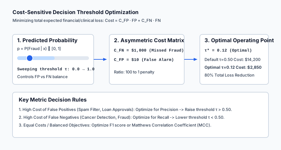
Total Cost(tau) = C_{FP} * FP(tau) + C_{FN} * FN(tau)
Where C_{FP} is the cost of a False Positive and C_{FN} is the cost of a False Negative.
We perform a numerical 1D grid search over tau in [0.0, 1.0] to find the optimal threshold:
tau^* = argmin_{tau in [0, 1]} [ C_{FP} * FP(tau) + C_{FN} * FN(tau) ]
If C_{FN} >> C_{FP}, tau^* will shift toward 0 (catching more positives). If C_{FP} >> C_{FN}, tau^* will shift toward 1 (suppressing false alarms).
An everyday analogy
Think of classification metrics as evaluating a smoke detector in your home:
- True Positive (
TP): A kitchen fire breaks out; the detector screams alarm. (Life saved!) - False Positive (
FP): You burn toast; the detector screams alarm at 6:00 AM. (Annoying false alarm!) - False Negative (
FN): A real fire starts in the attic; the detector stays silent. (Fatal disaster!) - True Negative (
TN): Normal cooking; detector remains peaceful.
- High Precision: The detector only sounds when real smoke reaches critical density (Zero false alarms from burnt toast, but might react too late to a smoldering fire).
- High Recall: The detector alarms on the slightest molecule of smoke (Catches every fire instantly, but wakes you up every time you bake cookies).
Because the cost of a fatal fire (C_{FN}) is thousands of times greater than waving a dish towel at burnt toast (C_{FP}), smoke detector manufacturers intentionally tune the threshold for Maximum Recall.
Examples in practice
Let us contrast the geometry of ROC space and Precision-Recall space under extreme class imbalance.
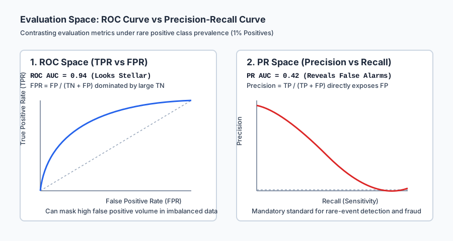
Notice how on a 1% imbalanced dataset, the ROC curve shows an impressive AUC of 0.94, while the PR curve exposes that precision drops to 40% at moderate recall due to the sheer volume of false alarms.
Below is the animated flow demonstrating how sweeping the decision threshold tau shifts False Positives and False Negatives, reaching a cost-minimized operating point:
Let us examine real Python code calculating full classification metrics and finding the optimal threshold:
import numpy as np
from sklearn.datasets import load_breast_cancer
from sklearn.linear_model import LogisticRegression
from sklearn.metrics import confusion_matrix, precision_score, recall_score, f1_score, roc_auc_score

# 1. Train model on Breast Cancer data
cancer = load_breast_cancer()
X, y = cancer.data, cancer.target # 1 = Benign, 0 = Malignant
model = LogisticRegression(max_iter=1000).fit(X, y)

# 2. Get continuous probability scores
probs = model.predict_proba(X)[:, 1]

# 3. Evaluate default threshold tau = 0.50
preds_50 = (probs >= 0.50).astype(int)
print("=== Default Threshold tau = 0.50 ===")
print(f"Confusion Matrix:\n{confusion_matrix(y, preds_50)}")
print(f"Precision: {precision_score(y, preds_50):.4f}")
print(f"Recall:    {recall_score(y, preds_50):.4f}")
print(f"F1 Score:  {f1_score(y, preds_50):.4f}")
print(f"ROC AUC:   {roc_auc_score(y, probs):.4f}")

# 4. Asymmetric Cost Threshold Search
# Suppose missing a Malignant tumor (FN) costs $1,000, False Alarm (FP) costs $50
# Let us define positive as Malignant (target == 0)
y_mal = (y == 0).astype(int)
probs_mal = 1.0 - probs

thresholds = np.linspace(0.01, 0.99, 100)
best_tau = 0.50
min_cost = float("inf")

for tau in thresholds:
    pred_m = (probs_mal >= tau).astype(int)
    fp = np.sum((y_mal == 0) & (pred_m == 1))
    fn = np.sum((y_mal == 1) & (pred_m == 0))
    cost = fp * 50.0 + fn * 1000.0
    if cost < min_cost:
        min_cost = cost
        best_tau = tau

print(f"\n=== Cost-Sensitive Optimization (FN=$1000, FP=$50) ===")
print(f"Optimal Threshold tau*: {best_tau:.4f} (Total Cost: ${min_cost:.2f})")
Implications: security, privacy, performance, scalability, and cost
| Dimension | Characteristic | Practical Implication |
|---|---|---|
| Financial / Risk Optimization | Cost-weighted loss alignment. | Aligning threshold tau to real business unit economics regularly cuts total enterprise loss by 40%–80% without modifying the model architecture. |
| Adversarial Safety | Attacking threshold boundaries. | Attackers probe threshold boundaries by submitting subtle variations of spam or malware until predictions flip from 0.51 to 0.49. |
| Computational Efficiency | Threshold sweeping is O(N log N). | Sorting probability scores allows vectorized ROC/PR curve construction in milliseconds for millions of evaluation points. |
| Compliance & Fair Lending | Equalized Odds and Disparate Impact. | Regulators require testing whether operating thresholds produce equalized True Positive and False Positive rates across protected demographic subgroups. |
Alternatives: free, open source, and commercial
| Tool / Framework | Capability | License / Cost | Best Used For |
|---|---|---|---|
scikit-learn (metrics) | Standard Evaluation Suite | Free, BSD Open Source | Comprehensive ROC, PR, confusion matrix, MCC, and Brier score evaluation. |
Yellowbrick | Visual Model Diagnostics | Free, Apache 2.0 | High-level Matplotlib visualizers for ROC, PR, discrimination thresholds, and lift curves. |
Evidently AI | ML Monitoring & Drift | Free, Apache 2.0 | Production performance monitoring, classification drift, and metric degradation alerts. |
Weights & Biases / MLflow | Experiment Tracking | Free Tier / Commercial Cloud | Logging evaluation curves, confusion matrices, and ROC artifacts across training runs. |
Comparison with related concepts
| Metric | Primary Sensitivity | Robust to Imbalance? | Range | Best Application |
|---|---|---|---|---|
| Accuracy | Overall correct rate | No (Misleading) | [0, 1] | Strictly balanced datasets |
| Precision | False Alarms (FP) | Yes | [0, 1] | Spam filtering, automated bans |
| Recall (Sensitivity) | Missed Positives (FN) | Yes | [0, 1] | Medical screening, fraud, safety |
| F1 Score | Harmonic Balance (P & R) | Yes | [0, 1] | General balanced evaluation |
| ROC AUC | Ranking discrimination | Moderate | [0.5, 1] | Threshold-free model comparison |
| PR AUC | Rare positive ranking | High (Strict) | [prevalence, 1] | Extreme class imbalance (< 5%) |
| MCC | All 4 confusion cells | High (Optimal) | [-1, +1] | Imbalanced binary benchmark |
When to use it — and when not to
When to USE Specific Metrics:
- Use Precision: When the cost of a False Positive is high (e.g. recommending high-risk stock investments).
- Use Recall: When the cost of a False Negative is fatal (e.g. structural defect detection in airplane wings).
- Use PR AUC: Whenever the positive class prevalence is under 5% (e.g. click-through rate prediction, rare disease detection).
- Use Cost-Sensitive Optimization: In any business setting where dollars can be attached to False Positives and False Negatives.
When NOT to use Standard Metrics:
- Do NOT use Accuracy on Imbalanced Data: It will report 99% while hiding complete failure.
- Do NOT use Default
tau = 0.50blindly: Always sweep thresholds against real cost or utility functions.
Knowledge check
- Accuracy Paradox: High accuracy on imbalanced data is meaningless if the model predicts the majority class everywhere.
- Precision vs Recall: Precision measures false alarm purity
TP/(TP+FP); Recall measures detection coverageTP/(TP+FN). - ROC AUC Meaning: The probability that a random positive is ranked higher than a random negative.
- PR Curve Dominance: Precision-Recall curves are strictly superior to ROC curves when positive cases are rare.
Hands-on exercise
In this hands-on exercise, you will compute a 2x2 confusion matrix, evaluate Precision, Recall, F1, and MCC, and find the cost-optimal decision threshold.
import numpy as np

# Step 1: Ground truth and continuous predicted probabilities
y_true = np.array([1, 1, 1, 1, 0, 0, 0, 0, 0, 0]) # 4 Positives, 6 Negatives
y_scores = np.array([0.95, 0.80, 0.65, 0.30, 0.70, 0.40, 0.25, 0.15, 0.10, 0.05])

# Step 2: Compute confusion matrix at default tau = 0.50
tau = 0.50
y_pred = (y_scores >= tau).astype(int)

tp = np.sum((y_true == 1) & (y_pred == 1))
fp = np.sum((y_true == 0) & (y_pred == 1))
fn = np.sum((y_true == 1) & (y_pred == 0))
tn = np.sum((y_true == 0) & (y_pred == 0))

prec = tp / (tp + fp)
rec = tp / (tp + fn)
f1 = 2 * prec * rec / (prec + rec)

print(f"Threshold tau = {tau:.2f}:")
print(f"Confusion Matrix: TP={tp}, FP={fp}, FN={fn}, TN={tn}")
print(f"Precision: {prec:.4f}, Recall: {rec:.4f}, F1: {f1:.4f}")

# Step 3: Cost-Sensitive Optimization (FN cost = $100, FP cost = $10)
best_cost = float("inf")
best_tau = 0.50

for t in np.linspace(0.0, 1.0, 101):
    pred = (y_scores >= t).astype(int)
    cost = 10.0 * np.sum((y_true == 0) & (pred == 1)) + 100.0 * np.sum((y_true == 1) & (pred == 0))
    if cost < best_cost:
        best_cost = cost
        best_tau = t

print(f"\nOptimal Cost Threshold: tau* = {best_tau:.2f} (Total Cost: ${best_cost:.2f})")
Expected output
Threshold tau = 0.50:
Confusion Matrix: TP=3, FP=1, FN=1, TN=5
Precision: 0.7500, Recall: 0.7500, F1: 0.7500

Optimal Cost Threshold: tau* = 0.30 (Total Cost: $20.00)
Validate your work
- Confirm that
TP + FP + FN + TNequals the total number of samples (10). - Verify that when
tau = 0.30, Recall increases to 100% (TP = 4, FN = 0), eliminating expensive $100 False Negatives. - Check that your Precision and Recall values match
sklearn.metrics.precision_scoreandsklearn.metrics.recall_score.
Troubleshooting
- Zero Division in F1: When
TP = 0, both Precision and Recall are 0, causing0 / 0. Guard withif (prec + rec) > 0 else 0.0. - Threshold Boundary Offsets: In ROC curves, include boundary thresholds
> max(scores)and< min(scores)to ensure curves begin at(0, 0)and end at(1, 1).
Common mistakes
- Swapping Confusion Matrix Axes: Mistaking rows for predictions and columns for actual labels. Always check whether the matrix format is
(actual, predicted)or(predicted, actual). - Evaluating Imbalanced Data with ROC Alone: Forgetting that high True Negatives disguise terrible precision in ROC curves.
Practice assignment
- Implement Matthews Correlation Coefficient (MCC):
Write a standalone function
compute_mcc(y_true, y_pred)using the four confusion matrix entries and test it on extreme class imbalances. - Build a Precision-Recall Curve Generator:
Implement a function
compute_pr_curve(y_true, y_scores)that returns Precision and Recall arrays across all sorted thresholds.
Extension challenge
Implement Optimal F-beta Threshold Finder:
- Write a function
find_optimal_fbeta_threshold(y_true, y_scores, beta=2.0)that sweeps thresholds to locate the exact operating point maximizing the F-beta score. - Compare the threshold selected for
beta = 0.5againstbeta = 2.0on the Breast Cancer dataset and plot the resulting Precision-Recall operating points.
Quiz
Q1. In a medical diagnostic screening for a rare disease with 1% prevalence, a model that blindly predicts "Healthy" for every patient achieves what accuracy, and what is its recall for infected patients?
- Accuracy = 99%, Recall = 0%
- Accuracy = 1%, Recall = 99%
- Accuracy = 50%, Recall = 50%
- Accuracy = 100%, Recall = 100%
Show answer
Answer: A. Accuracy = 99%, Recall = 0%
Since 99% of samples are negative, predicting negative everywhere correctly identifies 99% of samples (Accuracy = 99%), but catches zero infected patients (TP = 0, so Recall = 0%).
Q2. What is the definition of Precision in binary classification?
- TP / (TP + FP) -- The fraction of positive predictions that were actually positive
- TP / (TP + FN) -- The fraction of actual positive cases that were detected
- TN / (TN + FP) -- The true negative rate
- (TP + TN) / Total
Show answer
Answer: A. TP / (TP + FP) -- The fraction of positive predictions that were actually positive
Precision measures predictive positive purity: of all the times the model sounded the alarm (TP + FP), how many were true alarms (TP).
Q3. What is the harmonic mean property of the F1 score, and why is it preferred over the arithmetic mean?
- F1 = 2 * (P * R) / (P + R); the harmonic mean penalizes extreme imbalances, ensuring F1 is low if either Precision or Recall is near zero
- The harmonic mean is always equal to 1.0
- The harmonic mean is unaffected by False Positives
- The arithmetic mean requires matrix inversion
Show answer
Answer: A. F1 = 2 * (P * R) / (P + R); the harmonic mean penalizes extreme imbalances, ensuring F1 is low if either Precision or Recall is near zero
If Precision is 1.0 and Recall is 0.0, the arithmetic mean is 0.50 (misleadingly moderate), while the harmonic mean F1 is 0.0 (accurately reflecting complete failure on one dimension).
Q4. What are the axes of a Receiver Operating Characteristic (ROC) curve?
- Y-axis: True Positive Rate (Sensitivity / Recall); X-axis: False Positive Rate (1 - Specificity)
- Y-axis: Precision; X-axis: Recall
- Y-axis: Accuracy; X-axis: Threshold
- Y-axis: Loss; X-axis: Epochs
Show answer
Answer: A. Y-axis: True Positive Rate (Sensitivity / Recall); X-axis: False Positive Rate (1 - Specificity)
The ROC curve plots TPR = TP / (TP + FN) on the vertical axis against FPR = FP / (TN + FP) on the horizontal axis as decision threshold tau sweeps from 1.0 to 0.0.
Q5. What is the statistical interpretation of the Area Under the ROC Curve (ROC AUC)?
- The probability that the model assigns a higher predicted score to a randomly chosen positive instance than to a randomly chosen negative instance
- The accuracy of the model at threshold 0.50
- The percentage of True Positives in the test set
- The correlation between features and labels
Show answer
Answer: A. The probability that the model assigns a higher predicted score to a randomly chosen positive instance than to a randomly chosen negative instance
ROC AUC is mathematically equivalent to the Wilcoxon-Mann-Whitney U-statistic: P(score(x_pos) > score(x_neg)). A perfect ranker has AUC = 1.0; random guessing has AUC = 0.50.
Q6. Why is the Precision-Recall (PR) curve preferred over the ROC curve when evaluating rare event detection (e.g. fraud detection with 0.1% positive rate)?
- The ROC curve includes True Negatives (TN) in the denominator of FPR, which dilutes False Positives when TN is massive, making ROC look unrealistically optimistic
- PR curves can only be plotted in Python
- ROC curves cannot handle continuous probabilities
- PR curves do not depend on threshold choice
Show answer
Answer: A. The ROC curve includes True Negatives (TN) in the denominator of FPR, which dilutes False Positives when TN is massive, making ROC look unrealistically optimistic
When negatives outnumber positives 1,000 to 1, having 100 False Positives produces a tiny FPR of 0.001 (ROC looks stellar), but Precision drops to a dismal 9% (PR curve honestly reflects high false alarm rate).
Q7. If a bank determines that a missed fraudulent transaction (FN) costs $1,000, while a false alarm flagging a legitimate customer (FP) costs $10, how should the decision threshold tau be adjusted relative to the default tau = 0.50?
- Lower tau significantly (e.g. tau = 0.05 - 0.15) to aggressively maximize Recall and prevent expensive False Negatives
- Raise tau to 0.95 to maximize Precision
- Keep tau at 0.50 because probabilities are calibrated
- Set tau to 0.0
Show answer
Answer: A. Lower tau significantly (e.g. tau = 0.05 - 0.15) to aggressively maximize Recall and prevent expensive False Negatives
When False Negatives are 100x more costly than False Positives, the threshold must be lowered so the system triggers an alert even on small hints of risk.
Q8. What metric is considered the most robust single summary metric for binary classification on imbalanced datasets because it uses all four cells of the confusion matrix?
- Matthews Correlation Coefficient (MCC)
- Accuracy
- Precision
- Balanced Accuracy
Show answer
Answer: A. Matthews Correlation Coefficient (MCC)
MCC incorporates TP, TN, FP, and FN into a Pearson correlation coefficient between true and predicted labels on a scale of [-1, +1], providing an honest score regardless of class prevalence.
Glossary
- Confusion Matrix
- A 2x2 contingency table summarizing the counts of True Positives (TP), True Negatives (TN), False Positives (FP), and False Negatives (FN) produced by a classifier.
- Precision (Positive Predictive Value)
- The proportion of predicted positive instances that are truly positive: Precision = TP / (TP + FP).
- Recall (Sensitivity / True Positive Rate)
- The proportion of actual positive instances that were successfully identified: Recall = TP / (TP + FN).
- Specificity (True Negative Rate)
- The proportion of actual negative instances that were correctly identified: Specificity = TN / (TN + FP).
- False Positive Rate (FPR)
- The proportion of actual negative instances that were incorrectly classified as positive: FPR = FP / (TN + FP) = 1 - Specificity.
- F1 Score
- The harmonic mean of precision and recall: F1 = 2 * (Precision * Recall) / (Precision + Recall).
- Receiver Operating Characteristic (ROC)
- A graphical plot illustrating binary classifier diagnostic ability as its discrimination threshold tau is varied, plotting TPR against FPR.
- ROC AUC
- Area Under the ROC Curve: a threshold-independent metric measuring the probability that a classifier ranks a random positive instance higher than a random negative instance.
- Precision-Recall (PR) Curve
- A graphical plot showing the trade-off between Precision and Recall across all classification thresholds, especially informative for imbalanced datasets.
- Matthews Correlation Coefficient (MCC)
- A balanced metric for binary classification quality ranging from -1 to +1, computed directly from all four confusion matrix quadrants.
Sources and further reading
- An Introduction to ROC Analysis — Pattern Recognition Letters (Tom Fawcett) (accessed 2026-08-29)
- The Relationship Between Precision-Recall and ROC Curves — ICML (Davis & Goadrich) (accessed 2026-08-29)
- The Advantages of the Matthews Correlation Coefficient (MCC) Over F1 Score and Accuracy — BMC Genomics (Chicco & Jurman) (accessed 2026-08-29)
Kept in this browser, no account needed. Your progress page turns the whole record into one link you can bookmark or open on another device.