Machine Learning › Trees and Ensembles › Day 162
Day 162: Decision Trees
Master the theory, mathematics, and implementation of Decision Trees from first principles: why trees partition feature space into axis-aligned hyper-rectangles, how Gini impurity and Shannon entropy measure node homogeneity, how the CART algorithm searches greedily for optimal split thresholds, why unpruned trees suffer from high variance and overfitting, and how hyperparameter constraints and pruning restore generalization.
Hands-on lab for this lesson
Lab files on GitHub: https://github.com/ai-roadmap-365/ai-roadmap-365.github.io/tree/main/labs/sections/machine-learning/day-162-decision-trees
- Get the hands-on files. Clone the labs repository once (you can reuse this clone for every lesson). This works on macOS, Linux, and Windows (PowerShell or WSL):
git clone https://github.com/ai-roadmap-365/ai-roadmap-365.github.io.git cd ai-roadmap-365.github.io - Open this lesson's lab. Move into the directory for this specific day. Every lab lives at the same predictable path — section / subsection / week / day:
cd labs/sections/machine-learning/day-162-decision-trees - Read the lab guide. Open `README.md` in that directory. It lists the exact commands, what each does, the expected output, and how to check your work — read it before running anything.
- Run it and check your work. Follow the README's "How to run" section: run the example first to see the finished result, then complete the numbered exercises in `starter/`, then run the tests. The tests pass (exit 0) only when your work is correct.
bash tests/run_tests.sh # or the test command named in the lab README
You can also open the lab as a local page (works offline, shows the file tree and expected output).
Learning objectives
By the end of this lesson you will be able to:
- Explain how decision trees recursively partition continuous feature space into axis-aligned rectangular regions
- Derive and compute Gini Impurity, Shannon Entropy, and Information Gain
- Formulate the greedy CART split optimization objective function
- Implement a complete binary decision tree classifier from scratch using recursive tree structures
- Analyze the inductive bias, non-parametric nature, and scale invariance of decision trees
- Diagnose overfitting mechanisms in unconstrained trees and identify high-variance failure modes
- Apply pre-pruning hyperparameters (max_depth, min_samples_split, min_samples_leaf) to prevent memorization
- Benchmark custom decision trees against scikit-learn DecisionTreeClassifier on real multiclass data
Prerequisites
- Day 156 -- Decision boundaries and non-linear partitions
- Day 159 -- Classification metrics and confusion matrices
Why this matters
In Weeks 21 through 23, we studied linear models: linear regression, logistic regression, and their regularized variants. Linear models possess an undeniable elegance: they compute a weighted sum of inputs w^T x + b, evaluate a scalar threshold, and produce decisions with microsecond latency.
Yet linear models carry a severe structural limitation: they can only separate classes with flat, linear hyperplanes.
If your data contains non-linear interactions (for example, high blood pressure is only dangerous if cholesterol is also elevated), linear models require manual polynomial feature engineering. If your data contains categorical variables with complex hierarchies, linear models require high-dimensional one-hot encodings. If your features have vastly different scales (e.g. income in dollars vs age in years), linear models require standardizing scalers.
Decision Trees break free from these geometric restrictions entirely.
A decision tree is a non-parametric model that recursively partitions feature space into axis-aligned rectangular boxes. Trees automatically discover non-linear relationships and high-order feature interactions, accept numerical and categorical features without scaling, handle missing values seamlessly, and present their learned logic as human-readable if-then-else decision rules.
Furthermore, decision trees serve as the foundational atomic building blocks for the most powerful tabular learning algorithms in history: Random Forests (Day 163) and Gradient Boosted Trees (Days 164–165). Understanding how a single tree splits, grows, and overfits is the prerequisite for mastering all modern tabular machine learning.
The idea in plain language
Imagine playing a game of 20 Questions with a doctor who is diagnosing a patient:
- Question 1: “Is the patient’s resting heart rate above 100 beats per minute?”
- If No: The doctor moves down the left branch and asks: “Is body temperature above 38.5°C?”
- If Yes: The doctor moves down the right branch and asks: “Is blood oxygen saturation below 92%?”
Each question is a simple binary split on a single feature: x_j <= threshold.
As you follow the questions from the root of the tree down to the leaves, each step narrows down the diagnosis. When you reach a terminal leaf node, the tree makes a final prediction: “Class = Influenza” or “Class = Healthy”.
In geometric terms, each question draws an orthogonal, axis-aligned line across your feature space. Two questions carve the 2D plane into four rectangles; three questions carve 3D space into eight rectangular boxes. Inside each box, the tree predicts the majority class of the training samples that landed there.
Historical background
The conceptual origins of decision trees trace back to the Morgan and Sonquist 1963 Automatic Interaction Detection (AID) program.
In 1984, Leo Breiman, Jerome Friedman, Richard Olshen, and Charles Stone published their monumental book Classification and Regression Trees (CART). The CART framework introduced the modern algorithm used across machine learning: binary recursive splitting using Gini Impurity for classification, variance reduction for regression, and Cost-Complexity Pruning to regularize tree growth.
Concurrently in computer science, J. Ross Quinlan developed ID3 (Iterative Dichotomiser 3, 1986) and its successor C4.5 (1993), which used information theory and Shannon Entropy to evaluate multi-way splits.
In 2000, Breiman and Friedman’s insights culminated in ensemble tree algorithms that continue to dominate tabular Kaggle competitions and commercial predictive modeling pipelines worldwide.
What it is — and what it is not
To reason about decision trees with rigorous engineering clarity, let us define what a decision tree is and is not:
What it IS:
- A Non-Parametric Hierarchical Model: It makes no assumptions about the underlying distribution of data (unlike Gaussian Naive Bayes or linear models).
- An Axis-Aligned Space Partitioner: Every internal split evaluates a single feature inequality
x_j <= t, carving feature space into hyper-rectangles. - Scale Invariant: It depends strictly on the rank-order sorting of feature values. Standardizing, normalizing, or taking logarithms of features has zero impact on split locations.
- A Greedy Recursive Optimizer: At each node, CART finds the locally optimal single split that maximizes immediate impurity reduction, without looking ahead to future splits.
What it is NOT:
- Not Smooth or Differentiable: Decision tree predictions are piecewise-constant step functions. They cannot extrapolate smooth linear trends beyond the bounding box of the training data.
- Not a Global Optimizer: The greedy split selection cannot guarantee a globally optimal tree. Finding the optimal decision tree is mathematically NP-complete.
- Not Low-Variance: A single decision tree is notorious for high variance. Changing a single training sample can drastically alter the root split, creating an entirely different downstream tree structure.
Why it was created and what problems it solves
Decision trees solve five pervasive challenges in tabular machine learning:
- Automatic Discovery of Feature Interactions: If feature A only matters when feature B is true, a tree captures this interaction naturally by placing feature A’s split inside feature B’s subtree.
- Zero Feature Preprocessing Overhead: Trees require no scaling, no centering, no outlier clipping, and no monotonic transformations.
- Intrinsic Multi-Class Support:
Impurity metrics (Gini and Entropy) generalize naturally to
Kclasses without requiring One-vs-Rest or One-vs-One wrappers. - Complete Interpretability and Auditability: Every prediction can be explained by tracing a single deterministic path of if-then rules from root to leaf.
- Robust Non-Linear Modeling: Trees model complex non-linear decision boundaries with zero manual kernel expansions.
How it works
Let us formulate the mathematics of decision tree induction, impurity functions, greedy split selection, and regularization.
1. Impurity Metrics: Quantifying Node Homogeneity
Let node m contain N_m training samples belonging to K distinct classes. The empirical class probability distribution at node m is:
p_{mk} = (1 / N_m) * sum_{i in Q_m} I(y_i == k)
Where Q_m is the set of samples in node m, and sum_{k=1}^K p_{mk} = 1.0.
How do we measure whether node m is pure (all samples belong to one class) or mixed (samples are evenly scattered)?
A. Gini Impurity (CART Default)
Gini impurity measures the probability that a randomly chosen element from the set would be incorrectly labeled if it were randomly labeled according to the class distribution in the node:
G(Q_m) = 1 - sum_{k=1}^K p_{mk}^2 = sum_{k=1}^K p_{mk} (1 - p_{mk})
- Pure Node (All Class 1):
p_1 = 1.0 ==> G = 1 - (1.0)^2 = 0.0(Minimum Impurity). - Evenly Split Binary Node (50% / 50%):
p_1 = 0.5, p_2 = 0.5 ==> G = 1 - (0.25 + 0.25) = 0.50(Maximum Binary Impurity). - Evenly Split K-Class Node:
p_k = 1/K ==> G = 1 - K * (1/K)^2 = 1 - 1/K.
B. Shannon Entropy (Information Theory)
Shannon entropy measures the expected information (in bits) required to describe the class label of a sample in node m:
H(Q_m) = - sum_{k=1}^K p_{mk} * log_2(p_{mk})
- Pure Node:
H = - 1.0 * log_2(1.0) = 0.0 bits. - Evenly Split Binary Node:
H = - 2 * (0.5 * log_2(0.5)) = - 2 * (0.5 * (-1.0)) = 1.0 bit. - Evenly Split K-Class Node:
H = log_2(K) bits.
Gini and Entropy produce nearly identical split rankings in practice. Gini is computationally faster because it requires simple squarings rather than expensive logarithmic evaluations.
2. Greedy Split Selection in CART
At node m, we wish to find a split theta = (j, t) where j is a feature index (1 <= j <= D) and t is a real-valued scalar threshold (t in R).
The candidate split partitions the N_m samples into left and right child subsets:
Q_{left}(j, t) = { x in Q_m | x_j <= t }
Q_{right}(j, t) = { x in Q_m | x_j > t }
Let N_L = |Q_{left}| and N_R = |Q_{right}|, with N_L + N_R = N_m.
The weighted child impurity of split (j, t) is:
G(Q_m, j, t) = (N_L / N_m) * H(Q_{left}) + (N_R / N_m) * H(Q_{right})
The Impurity Reduction (Information Gain) is:
Delta H(m, j, t) = H(Q_m) - G(Q_m, j, t)
The CART algorithm evaluates all features j in {1, ..., D} and all candidate midpoint thresholds t, selecting the optimal split:
(j^*, t^*) = argmin_{j, t} G(Q_m, j, t) = argmax_{j, t} Delta H(m, j, t)
3. Recursive Tree Induction Algorithm
Algorithm: BuildTree(Data X, Labels y, current_depth)
1. Check Termination Base Cases:
   - If current_depth >= max_depth
   - Or len(y) < min_samples_split
   - Or all y belong to the same class (Impurity == 0.0)
   - Then Return LeafNode(class = MajorityClass(y))

2. Find Optimal Split:
   - (j*, t*, min_cost) = FindBestSplit(X, y)
   - If no valid split found (e.g. all features identical):
       Return LeafNode(class = MajorityClass(y))

3. Partition Data:
   - Left_Mask = (X[:, j*] <= t*)
   - Right_Mask = ~Left_Mask

4. Recursive Children:
   - LeftChild = BuildTree(X[Left_Mask], y[Left_Mask], current_depth + 1)
   - RightChild = BuildTree(X[Right_Mask], y[Right_Mask], current_depth + 1)

5. Return InternalNode(feature = j*, threshold = t*, Left = LeftChild, Right = RightChild)
4. Overfitting Mechanisms and Regularization
If left unconstrained, a decision tree will continue splitting until every single training sample occupies its own private leaf node (Gini = 0.0, 100% Training Accuracy).
An unpruned tree memorizes noisy training points, outliers, and spurious correlations, creating tiny, jagged decision regions that fail completely on unseen test data.
┌────────────────────────────────────────────────────────────────────────┐
│               DECISION TREE REGULARIZATION TECHNIQUES                  │
├────────────────────────────────────────────────────────────────────────┤
│ 1. max_depth: Limits tree height (e.g. depth 3 to 6).                  │
│ 2. min_samples_split: Minimum samples required to attempt a split.    │
│ 3. min_samples_leaf: Minimum samples required in any leaf node.        │
│ 4. max_leaf_nodes: Maximum total number of terminal leaves allowed.   │
│ 5. ccp_alpha: Minimal Cost-Complexity Pruning penalty.                 │
└────────────────────────────────────────────────────────────────────────┘
Cost-Complexity Pruning (ccp_alpha):
Finds the subtree T that minimizes the penalized cost function:
R_alpha(T) = R(T) + alpha * |T|
Where R(T) is the total misclassification rate of tree T, |T| is the number of terminal leaf nodes, and alpha >= 0 is the complexity parameter governing the trade-off between tree size and fit quality.
An everyday analogy
Think of a decision tree as an expert game of 20 Questions:
- The Root Question: The player asks the single question that splits the universe of possibilities in half with maximum certainty (“Is it alive?”).
- The Branching Logic: Depending on the answer, the next question adapts entirely (“Is it an animal?” vs “Is it made of metal?”).
- The Leaf Conclusion: After 5 or 6 well-chosen questions, the player arrives at a high-confidence answer (“It is a Golden Retriever”).
- The Overfitting Danger: If the player is allowed 1,000 questions, they will ask: “Was it sitting on the corner of 5th and Main at 3:14 PM yesterday wearing a blue collar?” This question perfectly identifies the specific dog in the training sample, but fails to recognize any other dog in the world.
Examples in practice
Let us visualize the equivalence between binary tree hierarchies and orthogonal 2D feature space partitioning.
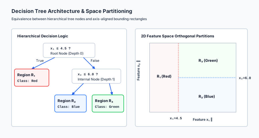
The diagram contrasts hierarchical branching rules with the geometric bounding boxes carved out in feature space.
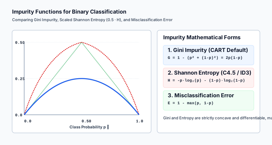
Below is the comparison between Gini Impurity, Scaled Shannon Entropy, and Misclassification Error:
Let us examine real Python code fitting a decision tree from scratch and comparing it against scikit-learn:
import numpy as np
from sklearn.datasets import load_iris
from sklearn.tree import DecisionTreeClassifier
from sklearn.model_selection import train_test_split
from sklearn.metrics import accuracy_score

# 1. Load Iris Data
iris = load_iris()
X, y = iris.data, iris.target

X_train, X_test, y_train, y_test = train_test_split(
    X, y, test_size=0.30, stratify=y, random_state=42
)

# 2. Fit Decision Tree with Depth Constraint
tree_clf = DecisionTreeClassifier(
    criterion="gini",
    max_depth=3,
    min_samples_split=4,
    min_samples_leaf=2,
    random_state=42
)
tree_clf.fit(X_train, y_train)

# 3. Evaluate Predictions
train_acc = accuracy_score(y_train, tree_clf.predict(X_train))
test_acc = accuracy_score(y_test, tree_clf.predict(X_test))

print("=== Decision Tree Performance ===")
print(f"Training Accuracy: {train_acc * 100:.2f}%")
print(f"Test Accuracy:     {test_acc * 100:.2f}%")
print(f"Tree Depth:        {tree_clf.get_depth()}")
print(f"Number of Leaves:  {tree_clf.get_n_leaves()}")
print("\nFeature Importances (MDI):")
for name, imp in zip(iris.feature_names, tree_clf.feature_importances_):
    print(f"• {name:20s}: {imp:.4f}")
Implications: security, privacy, performance, scalability, and cost
| Dimension | Characteristic | Practical Implication |
|---|---|---|
| Inference Latency & Cost | O(depth) integer comparisons. | Evaluating a decision tree involves 3 to 10 numerical comparisons, executing in < 10 microseconds with zero matrix multiplications. |
| Training Complexity | O(D * N * log N * depth). | Finding splits requires sorting feature columns. On massive datasets (N > 10M), training a single tree can become memory-intensive. |
| Data Privacy & Leakage | Single-sample leaf memorization. | In unpruned trees, individual leaf nodes can isolate single private records, allowing attackers to infer sensitive user attributes. |
| Explainability & Compliance | Full rule extraction. | Tree logic can be exported directly into SQL CASE WHEN statements, satisfying strict regulatory transparency requirements. |
Alternatives: free, open source, and commercial
| Tool / Framework | Architecture | License / Cost | Best Used For |
|---|---|---|---|
scikit-learn (DecisionTreeClassifier) | Optimized C-accelerated CART | Free, BSD Open Source | Baseline tree modeling, fast prototyping, and visualization with plot_tree. |
XGBoost / LightGBM / CatBoost | Boosted Tree Ensembles | Free, Apache / MIT | Production tabular modeling; combines hundreds of shallow trees for state-of-the-art accuracy. |
treelite | Tree Model Compiler | Free, Apache 2.0 | Compiling tree models into standalone C code for microsecond edge deployment. |
RuleFit | Rule-Extraction Sparse Linear Models | Free, Open Source | Extracting linear sparse combinations of tree decision rules for high interpretability. |
Comparison with related concepts
| Characteristic | Linear / Logistic Regression | k-Nearest Neighbors (KNN) | Single Decision Tree |
|---|---|---|---|
| Decision Boundary | Flat linear hyperplane | Complex curved Voronoi cells | Axis-aligned rectangular boxes |
| Feature Scaling | Strictly required | Strictly required | Not required (Scale invariant) |
| Interpretability | High (Weights w_j) | Low (Black box distances) | High (If-then rule paths) |
| Non-Linear Relationships | Requires manual interactions | Natural non-linear fitting | Natural non-linear fitting |
| Variance / Overfitting | Low variance | Sensitive to k | Very high variance (Needs pruning) |
When to use it — and when not to
When to USE a Single Decision Tree:
- Maximum Interpretability is Required: When business stakeholders or regulators require human-auditable if-then rules.
- Fast Exploratory Baseline: To quickly discover key feature interactions without data scaling.
- Edge Devices with Constrained Compute: Where model size must be
< 50 KBand evaluate without linear algebra libraries.
When NOT to use a Single Decision Tree:
- When Maximum Predictive Accuracy is Needed: A single tree is almost always beaten by ensembles (Random Forests, XGBoost).
- Linear or Diagonal Trends: Trees approximate diagonal hyperplanes with jagged step functions, requiring excessive depth.
- Continuous Extrapolation: Trees output constant step values outside the training bounding box and cannot extrapolate trends.
Knowledge check
- Axis-Aligned Splits: Trees evaluate
x_j <= t, creating orthogonal rectangular boundaries. - Gini vs Entropy:
G = 1 - sum(p_k^2)is fast and polynomial;H = - sum(p_k log2 p_k)is information-theoretic. - Scale Invariance: Trees depend solely on rank ordering; feature scaling has zero effect.
- Regularization:
max_depth,min_samples_split, andccp_alphaprevent leaf-level memorization.
Hands-on exercise
In this hands-on exercise, you will compute Gini impurity, find the optimal split on a 2D dataset, and construct a recursive binary tree node.
import numpy as np

# Step 1: Implement Gini Impurity
def gini(y):
    if len(y) == 0:
        return 0.0
    _, counts = np.unique(y, return_counts=True)
    return float(1.0 - np.sum((counts / len(y)) ** 2))

print("Gini of pure node [0, 0, 0]:", gini(np.array([0, 0, 0])))
print("Gini of balanced node [0, 1]:", gini(np.array([0, 1])))
print("Gini of 70/30 split:", gini(np.array([0]*7 + [1]*3)))

# Step 2: Optimal Split Search
X = np.array([[1.0, 5.0], [2.0, 6.0], [5.0, 2.0], [6.0, 1.0]])
y = np.array([0, 0, 1, 1])

def find_best_split(X, y):
    N, D = X.shape
    best_feat, best_t, best_cost = -1, 0.0, float("inf")
    for j in range(D):
        vals = np.unique(X[:, j])
        threshs = (vals[:-1] + vals[1:]) / 2.0
        for t in threshs:
            l_mask = X[:, j] <= t
            r_mask = ~l_mask
            cost = (np.sum(l_mask)/N) * gini(y[l_mask]) + (np.sum(r_mask)/N) * gini(y[r_mask])
            if cost < best_cost:
                best_cost, best_feat, best_t = cost, j, t
    return best_feat, best_t, best_cost

feat, thresh, cost = find_best_split(X, y)
print(f"\nOptimal Split: Feature x_{feat} <= {thresh:.2f} (Weighted Gini = {cost:.4f})")
Expected output
Gini of pure node [0, 0, 0]: 0.0
Gini of balanced node [0, 1]: 0.5
Gini of 70/30 split: 0.42

Optimal Split: Feature x_0 <= 3.50 (Weighted Gini = 0.0000)
Validate your work
- Verify that
gini([0, 1]) == 0.50andgini([0, 1, 2]) == 2/3. - Confirm that
find_best_splitreturnsfeat = 0andthreshold = 3.50withGini = 0.0. - Verify that fitting
DecisionTreeClassifier(max_depth=3)achieves>= 95%accuracy on Iris.
Troubleshooting
- Empty Split Mask: Ensure you skip thresholds where
sum(l_mask) == 0orsum(r_mask) == 0. - Single Unique Value in Column: Check
len(np.unique(X[:, j])) >= 2before computing midpoint thresholds.
Common mistakes
- Normalizing Features Before Trees: Unnecessary computation that provides zero accuracy benefit.
- Growing Unconstrained Trees: Forgetting
max_depthormin_samples_leafleads to severe test-set overfitting.
Practice assignment
- Implement Regression Trees (Variance Reduction):
Replace Gini impurity with Mean Squared Error
MSE = (1/N) * sum (y_i - y_bar)^2and build a decision tree regressor from scratch. - Implement Feature Importance Calculation:
Traverse a fitted tree and compute Mean Decrease in Impurity (MDI) for each feature by summing the impurity drops
N_m * Delta H(m)across all internal nodes.
Extension challenge
Implement Minimal Cost-Complexity Pruning from Scratch:
- Implement the weakest-link pruning algorithm that iteratively collapses internal nodes with the smallest effective alpha
g(t) = (R(t) - R(T_t)) / (|T_t| - 1). - Generate the cost-complexity pruning path
(alpha_1, ..., alpha_k)and use 5-fold cross-validation to select the optimal pruning parameteralpha^*.
Quiz
Q1. What is the geometric nature of the decision boundary produced by a standard single-feature Decision Tree?
- A piecewise-constant, axis-aligned orthogonal step boundary separating feature space into hyper-rectangles
- A smooth diagonal linear hyperplane
- A set of concentric circular Voronoi cells
- A high-degree smooth polynomial curve
Show answer
Answer: A. A piecewise-constant, axis-aligned orthogonal step boundary separating feature space into hyper-rectangles
Because each internal tree node splits on a single feature using an inequality x_j <= t, all decision boundaries are strictly orthogonal (perpendicular) to the feature axes.
Q2. What is the Gini Impurity of a binary classification node containing 70 Positive samples and 30 Negative samples?
- G = 1 - (0.7^2 + 0.3^2) = 1 - (0.49 + 0.09) = 0.42
- G = 0.70
- G = 0.50
- G = 0.21
Show answer
Answer: A. G = 1 - (0.7^2 + 0.3^2) = 1 - (0.49 + 0.09) = 0.42
Gini impurity is defined as 1 - sum(p_k^2). Here, p_pos = 0.7 and p_neg = 0.3, so G = 1 - (0.49 + 0.09) = 1 - 0.58 = 0.42.
Q3. Why are Decision Trees completely invariant to monotonic feature transformations (e.g. scaling, log-transforms, standardizing)?
- Because split evaluation depends solely on the relative rank ordering of feature values; transforming x to log(x) or 100*x preserves the exact same sample ordering and split point
- Because trees multiply all inputs by a learned weight matrix
- Because the Gini formula normalizes all values to [0, 1]
- Because decision trees only accept categorical variables
Show answer
Answer: A. Because split evaluation depends solely on the relative rank ordering of feature values; transforming x to log(x) or 100*x preserves the exact same sample ordering and split point
Tree splits evaluate inequalities like x_j <= t based on sample sorting. Any monotonic transformation preserves rank order, leaving the tree structure and predictions completely unchanged.
Q4. What is the primary fundamental weakness (failure mode) of an unconstrained, deeply grown Decision Tree?
- High variance and severe overfitting: an unpruned tree will grow until every leaf contains a single sample, memorizing noise and training artifacts
- High bias: the tree cannot fit non-linear patterns
- Extreme sensitivity to feature scaling
- Inability to handle multiclass classification
Show answer
Answer: A. High variance and severe overfitting: an unpruned tree will grow until every leaf contains a single sample, memorizing noise and training artifacts
Without stopping criteria or pruning, a decision tree will split until every training point is isolated in its own pure leaf, achieving 100% training accuracy but failing to generalize to new data.
Q5. How does the CART algorithm select the best feature j* and threshold t* at an internal node m?
- It exhaustively evaluates all features and candidate split thresholds, selecting the pair (j*, t*) that minimizes the weighted sum of child node impurities: (N_L / N_m) * Impurity(L) + (N_R / N_m) * Impurity(R)
- It computes the gradient of log-loss with respect to feature weights
- It randomly selects a feature and places the threshold at the median
- It solves the normal equation (X^T X)^-1 X^T y
Show answer
Answer: A. It exhaustively evaluates all features and candidate split thresholds, selecting the pair (j*, t*) that minimizes the weighted sum of child node impurities: (N_L / N_m) * Impurity(L) + (N_R / N_m) * Impurity(R)
CART is a greedy recursive partitioning algorithm that evaluates all possible midpoint thresholds across all features to minimize the weighted child impurity at each step.
Q6. What is the maximum possible value of Gini Impurity for a K-class classification problem?
- G_max = 1 - (1/K)
- G_max = 1.0
- G_max = K
- G_max = log2(K)
Show answer
Answer: A. G_max = 1 - (1/K)
When all K classes are equally likely (p_k = 1/K for all k), Gini impurity reaches its maximum: G_max = 1 - sum_{k=1}^K (1/K)^2 = 1 - K * (1/K^2) = 1 - (1/K).
Q7. What is the difference between Pre-Pruning (early stopping) and Post-Pruning (cost-complexity pruning)?
- Pre-pruning halts tree growth during training using hyperparameter limits (max_depth, min_samples_leaf); post-pruning grows a full tree first and then collapses subtrees that contribute less impurity reduction than penalty alpha
- Pre-pruning applies to classification; post-pruning applies to regression
- Pre-pruning uses Gini; post-pruning uses Entropy
- There is no mathematical difference
Show answer
Answer: A. Pre-pruning halts tree growth during training using hyperparameter limits (max_depth, min_samples_leaf); post-pruning grows a full tree first and then collapses subtrees that contribute less impurity reduction than penalty alpha
Pre-pruning stops splitting early (which can suffer from premature stopping when complex interactions require multiple splits). Post-pruning builds the full tree and prunes back weak branches using cost-complexity optimization.
Q8. Why is it difficult for a standard Decision Tree to model a simple diagonal linear boundary like x_1 + x_2 = 1?
- Because the tree can only make axis-aligned vertical and horizontal splits, forcing it to approximate the smooth diagonal line with a jagged staircase of many rectangular splits
- Because decision trees cannot compute addition
- Because linear boundaries require negative thresholds
- Because diagonal lines have zero Gini impurity
Show answer
Answer: A. Because the tree can only make axis-aligned vertical and horizontal splits, forcing it to approximate the smooth diagonal line with a jagged staircase of many rectangular splits
Axis-aligned splits must approximate continuous diagonal lines using a high-variance staircase approximation, requiring dozens of deep nodes where a single logistic regression hyperplane would suffice.
Glossary
- Decision Tree
- A non-parametric hierarchical supervised learning model that recursively partitions feature space into axis-aligned rectangular regions based on feature threshold tests.
- Gini Impurity
- A measure of node label heterogeneity in classification trees: G = 1 - sum(p_k^2), equal to 0.0 for pure nodes and maximized for uniform distributions.
- Shannon Entropy
- An information-theoretic measure of uncertainty: H = - sum(p_k * log2(p_k)), measuring the expected bits required to encode class labels.
- Information Gain
- The reduction in entropy achieved by partitioning a node into child subsets: IG = H(Parent) - sum((N_child / N_parent) * H(Child)).
- CART (Classification and Regression Trees)
- The standard greedy binary recursive partitioning algorithm developed by Breiman et al. using Gini impurity for classification and variance reduction for regression.
- Leaf Node
- A terminal node in a decision tree that contains no child branches and assigns a final class prediction (or continuous average) to all arriving samples.
- Axis-Aligned Split
- A decision rule evaluating a single feature against a scalar threshold (x_j <= t), creating boundaries strictly orthogonal to coordinate axes.
- Pre-Pruning (Early Stopping)
- Regularizing a decision tree by halting recursive growth when predefined stopping thresholds (max_depth, min_samples_split) are met.
- Cost-Complexity Pruning
- A post-pruning technique that minimizes a cost function balancing tree misclassification error against tree size parameterized by alpha.
- Scale Invariance
- The property of decision trees where monotonic feature transformations (e.g. scaling or log-transforms) have zero effect on split choices or model predictions.
Sources and further reading
- Classification and Regression Trees — CRC Press / Wadsworth (Breiman, Friedman, Olshen, Stone) (accessed 2026-08-29)
- Induction of Decision Trees — Machine Learning (J. Ross Quinlan) (accessed 2026-08-29)
- Scikit-Learn User Guide: Decision Trees — Scikit-Learn Developers (accessed 2026-08-29)
Kept in this browser, no account needed. Your progress page turns the whole record into one link you can bookmark or open on another device.