Machine Learning › Trees and Ensembles › Day 163
Day 163: Random Forests
Master the theory, mathematics, and implementation of Random Forests: why ensembling reduces model variance without increasing bias, how Bootstrap Aggregation (Bagging) samples data with replacement, why random feature subspace selection decorrelates individual trees, how Out-of-Bag (OOB) error provides free cross-validation, and how Random Forests achieve industry-standard tabular accuracy.
Hands-on lab for this lesson
Lab files on GitHub: https://github.com/ai-roadmap-365/ai-roadmap-365.github.io/tree/main/labs/sections/machine-learning/day-163-random-forests
- Get the hands-on files. Clone the labs repository once (you can reuse this clone for every lesson). This works on macOS, Linux, and Windows (PowerShell or WSL):
git clone https://github.com/ai-roadmap-365/ai-roadmap-365.github.io.git cd ai-roadmap-365.github.io - Open this lesson's lab. Move into the directory for this specific day. Every lab lives at the same predictable path — section / subsection / week / day:
cd labs/sections/machine-learning/day-163-random-forests - Read the lab guide. Open `README.md` in that directory. It lists the exact commands, what each does, the expected output, and how to check your work — read it before running anything.
- Run it and check your work. Follow the README's "How to run" section: run the example first to see the finished result, then complete the numbered exercises in `starter/`, then run the tests. The tests pass (exit 0) only when your work is correct.
bash tests/run_tests.sh # or the test command named in the lab README
You can also open the lab as a local page (works offline, shows the file tree and expected output).
Learning objectives
By the end of this lesson you will be able to:
- Derive the mathematical variance reduction formula for an ensemble of correlated estimators
- Explain Bootstrap Aggregation (Bagging) and prove that 36.8% of samples are Out-of-Bag
- Analyze why random feature subspace selection (max_features = sqrt(D)) decorrelates trees
- Implement a complete Random Forest Classifier from scratch in NumPy with majority voting
- Calculate Out-of-Bag (OOB) accuracy and explain why it eliminates the need for a separate validation split
- Contrast Mean Decrease in Impurity (MDI) with Permutation Feature Importance
- Compare Random Forests against single Decision Trees across bias, variance, and computational complexity
- Benchmark custom Random Forests against scikit-learn on high-dimensional clinical tabular data
Prerequisites
- Day 162 -- Decision Trees and CART splitting
- Day 152 -- Bias-Variance Trade-off
Why this matters
In Day 162, we discovered the immense expressive power and critical vulnerability of a single Decision Tree. While a decision tree can carve out intricate non-linear decision boundaries without feature scaling, it is notoriously unstable: an unpruned tree exhibits massive variance. Changing a single sample in the training set can completely alter the root split, cascading down into a wildly different downstream tree and generating brittle, overfit predictions.
How do we eliminate the high variance of decision trees while retaining their ability to model non-linear interactions?
The answer is Random Forests, conceived by Leo Breiman in 2001.
A Random Forest is an ensemble of dozens or hundreds of deep, high-variance decision trees. By combining Bootstrap Aggregation (Bagging) with Random Feature Subspace selection, Random Forests force the individual trees to be diverse and decorrelated. When you average the predictions of hundreds of decorrelated trees, their individual errors cancel out mathematically, driving model variance down to near zero while preserving the low bias of deep trees.
For over two decades, Random Forests have remained the gold standard baseline for tabular machine learning: robust to outliers, virtually immune to overfitting, requiring minimal hyperparameter tuning, and providing built-in cross-validation through Out-of-Bag (OOB) error estimation.
The idea in plain language
Imagine you want to diagnose a rare medical condition.
If you consult a single doctor (a single Decision Tree), they might be brilliant, but their diagnosis could be swayed by an unusual patient they treated yesterday. Their individual judgment carries high variance.
Now imagine consulting a panel of 100 independent doctors (a Random Forest):
- Diverse Experience (Bagging): Each doctor studied at a slightly different hospital and examined a randomized subset of medical case records.
- Diverse Questions (Random Subspaces): When interviewing the patient, each doctor is given a randomly restricted list of diagnostic tests. Doctor 1 looks at blood pressure and glucose; Doctor 2 looks at oxygen levels and ECG; Doctor 3 looks at genetics and age. This prevents all 100 doctors from focusing solely on the same single obvious symptom.
- Democratic Majority Vote: After all 100 doctors examine the patient independently, they cast their votes. If 88 doctors vote “Condition A” and 12 vote “Condition B”, the consensus prediction is “Condition A”.
The consensus of 100 diverse, decorrelated experts is vastly more reliable and robust than the opinion of any single expert.
Historical background
The theoretical foundation of ensembling began with Condorcet’s Jury Theorem in 1785, which proved mathematically that if each juror has a probability p > 0.5 of making a correct decision independently, the probability that the majority vote is correct approaches 1.0 as the jury size grows.
In 1996, Leo Breiman published Bagging Predictors, demonstrating that training estimators on bootstrap replicates of training data significantly reduces variance for unstable models like decision trees and neural networks, but does not help stable models like linear regression.
Concurrently in 1995, Tin Kam Ho at Bell Labs introduced the Random Subspace Method, showing that restricting trees to random subsets of features increases ensemble diversity.
In 2001, Breiman unified bagging, random feature subspaces, and out-of-bag error estimation in his seminal paper Random Forests. Breiman’s algorithm required no gradient descent, no learning rate schedules, and no feature scalers, instantly becoming one of the most widely deployed algorithms in industry.
What it is — and what it is not
To engineer with Random Forests effectively, we must define their exact characteristics:
What it IS:
- A Bagged Ensemble of Randomized Trees: An ensemble of
Bfully grown or deep decision trees trained on independent bootstrap samples. - A Variance Reduction Machine: It reduces variance by
1/Bwithout increasing individual tree bias. - A Parallel / Embarrassingly Parallel Algorithm: All
Btrees are completely independent and can be trained simultaneously across all available CPU cores. - A Self-Validating Model: Provides unbiased out-of-bag error estimates without requiring a separate train/validation split.
What it is NOT:
- Not a Boosting Algorithm: Trees are trained independently in parallel, NOT sequentially to correct previous errors (which is Gradient Boosting, Day 164).
- Not an Extrapolator: A Random Forest outputs the average of leaf predictions; it cannot extrapolate linear trends beyond the minimum and maximum target values observed in the training data.
- Not Compact in Memory: Storing 500 deep decision trees can require gigabytes of RAM compared to a compact vector of linear model weights.
Why it was created and what problems it solves
Random Forests solve five critical failure modes of single decision trees:
- Eliminates High Variance and Instability: Averaging
Bdecorrelated trees smooths out jagged step-function boundaries into smooth, probabilistic contours. - Immunity to Overfitting from Tree Count: Adding more trees (
n_estimators) does not cause overfitting; it monotonically stabilizes predictions until variance reaches its theoretical lower bound. - No Separate Validation Split Required: The Out-of-Bag (OOB) mechanism provides free, unbiased validation metrics on the training set.
- Resilience to Dominant Spurious Features: Random feature subsampling (
max_features = sqrt(D)) prevents a single dominant feature from dictating every tree’s root split. - Handles High-Dimensional Tabular Data Gracefully: Excels when
D > N(e.g. genomics or text embeddings) where linear models struggle with collinearity.
How it works
Let us formulate the mathematics of ensemble variance reduction, bootstrap sampling, random subspaces, and OOB error estimation.
1. The Mathematical Variance of an Ensemble
Consider an ensemble of B identically distributed (but not necessarily independent) base estimators f_1(x), f_2(x), ..., f_B(x).
Let each base estimator have variance Var(f_b(x)) = sigma^2, and let the pairwise correlation between any two distinct estimators be:
rho = Corr(f_i(x), f_j(x)) for all i != j
The ensemble prediction is the simple average:
bar{f}(x) = (1 / B) * sum_{b=1}^B f_b(x)
The variance of the ensemble average is derived as:
Var(bar{f}(x)) = Var( (1 / B) * sum_{b=1}^B f_b(x) )
= (1 / B^2) * [ sum_{b=1}^B Var(f_b(x)) + sum_{i != j} Cov(f_i(x), f_j(x)) ]
= (1 / B^2) * [ B * sigma^2 + B * (B - 1) * rho * sigma^2 ]
= rho * sigma^2 + ((1 - rho) / B) * sigma^2
Let us analyze this fundamental formula:
- If estimators are perfectly correlated (
rho = 1.0):Var(bar{f}(x)) = 1.0 * sigma^2 + 0 = sigma^2(Zero variance reduction!). - If estimators are completely independent (
rho = 0.0):Var(bar{f}(x)) = (1 / B) * sigma^2(Variance drops linearly to zero asB -> infinity). - In Practice (
0 < rho < 1): AsB -> infinity, the second term((1 - rho) / B) * sigma^2approaches0.0. The remaining irreducible ensemble variance is:lim_{B -> inf} Var(bar{f}(x)) = rho * sigma^2
Crucial Takeaway: To minimize ensemble variance, we must make rho (the correlation between trees) as small as possible!
2. Bootstrap Aggregation (Bagging)
How do we make trees different from one another?
Given a training dataset D = { (x_1, y_1), ..., (x_N, y_N) } of size N, we generate a bootstrap sample D_b of size N by sampling uniformly at random with replacement.
Original Data (N=4):  [A, B, C, D]
Bootstrap Bag 1:      [A, A, C, D]  (B is Out-of-Bag)
Bootstrap Bag 2:      [B, C, C, D]  (A is Out-of-Bag)
Bootstrap Bag 3:      [A, B, B, D]  (C is Out-of-Bag)
What fraction of samples are left out (Out-of-Bag)?
For a specific sample x_i, the probability of NOT being selected in a single random draw is:
P(not selected in 1 draw) = 1 - (1 / N)
Because the N draws in a bootstrap sample are independent, the probability that x_i is NOT selected in any of the N draws is:
P(x_i in OOB) = (1 - (1 / N))^N
Taking the calculus limit as dataset size N -> infinity:
lim_{N -> inf} (1 - (1 / N))^N = (1 / e) approx 0.367879...
Result: In every bootstrap sample, approximately 63.2% of original samples are selected (some repeated), and 36.8% of samples are left completely untouched (Out-of-Bag).
3. Random Feature Subspaces (Tree Decorrelation)
Standard bagging reduces correlation rho, but not enough if the dataset has strong features.
If feature x_1 is overwhelmingly predictive, every single bagged tree will choose x_1 as its root split. The resulting trees will look almost identical, keeping rho high and limiting variance reduction.
Leo Breiman’s breakthrough was to inject feature-level randomization:
At EVERY internal node split in EVERY tree:
1. Randomly sample a subset of m candidate features WITHOUT replacement:
   - For Classification: m = floor(sqrt(D))
   - For Regression:     m = floor(D / 3)
2. Evaluate candidate splits ONLY among those m features.
3. Select the best (feature, threshold) pair from the subset.
By restricting each split to sqrt(D) features, strong features are excluded in 1 - (sqrt(D) / D) fraction of splits, forcing trees to explore alternative predictive features and driving pairwise correlation rho down dramatically.
4. Out-of-Bag (OOB) Error Estimation
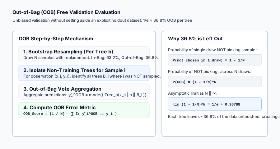
Because 36.8% of trees never saw sample i during training, we can evaluate sample i using only those trees:
Let B_i = { b in {1, ..., B} | (x_i, y_i) notin D_b } be the set of trees where sample i was out-of-bag.
The Out-of-Bag ensemble prediction for sample i is:
hat{y}_i^{OOB} = argmax_k sum_{b in B_i} I( Tree_b(x_i) == k )
The Out-of-Bag Accuracy (OOB Score) is:
OOB_Score = (1 / N) * sum_{i=1}^N I( hat{y}_i^{OOB} == y_i )
Engineering Benefit: The OOB score is an unbiased estimate of generalization error that is virtually identical to 5-fold cross-validation, but requires zero extra training runs.
An everyday analogy
Think of a Random Forest as an investigative journalist consortium:
- Individual Journalists (Single Trees): If a single journalist investigates a corporation, their report might be brilliant but biased by the specific sources they interviewed.
- Diverse Source Pools (Bagging): The editor sends 50 journalists into the field. Each journalist receives a different randomized set of confidential documents.
- Restricted Angles (Random Subspaces): Journalist A is only allowed to investigate accounting records; Journalist B is only allowed to interview former engineers; Journalist C is only allowed to inspect public permits. No single journalist can dominate the story with a single narrative.
- The Joint Editorial Consensus (Majority Voting): When all 50 independent reports are compiled, the consortium publishes only the facts corroborated by the majority. Outliers and false leads cancel out.
Examples in practice
Let us visualize the complete Random Forest architecture and data flow:
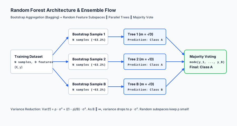
The diagram traces data from bootstrap resampling through randomized tree induction to final majority voting.
Below is the flow of Out-of-Bag (OOB) evaluation:
Let us examine real Python code training a Random Forest with OOB estimation and evaluating feature importances:
import numpy as np
from sklearn.datasets import load_breast_cancer
from sklearn.ensemble import RandomForestClassifier
from sklearn.model_selection import train_test_split
from sklearn.metrics import accuracy_score, classification_report

# 1. Load Clinical Tabular Dataset
cancer = load_breast_cancer()
X, y = cancer.data, cancer.target

X_train, X_test, y_train, y_test = train_test_split(
    X, y, test_size=0.25, stratify=y, random_state=42
)

# 2. Fit Random Forest with OOB Evaluation
rf = RandomForestClassifier(
    n_estimators=100,
    max_depth=8,
    max_features="sqrt",
    oob_score=True,
    n_jobs=-1, # Train across all CPU cores in parallel
    random_state=42
)
rf.fit(X_train, y_train)

# 3. Evaluate Generalization and OOB Match
test_acc = accuracy_score(y_test, rf.predict(X_test))

print("=== Random Forest Clinical Benchmark ===")
print(f"OOB Generalization Score: {rf.oob_score_ * 100:.2f}%")
print(f"Independent Test Accuracy: {test_acc * 100:.2f}%")
print(f"Number of Trees:           {len(rf.estimators_)}")

# 4. Inspect Top 5 Feature Importances (MDI)
importances = rf.feature_importances_
top_indices = np.argsort(importances)[::-1][:5]
print("\nTop 5 Most Predictive Features (MDI):")
for idx in top_indices:
    print(f"• {cancer.feature_names[idx]:25s}: {importances[idx]:.4f}")
Implications: security, privacy, performance, scalability, and cost
| Dimension | Characteristic | Practical Implication |
|---|---|---|
Training Scalability (n_jobs) | Embarrassingly parallel across CPU cores. | Training 500 trees on an 8-core CPU achieves a ~7.5x linear speedup with zero inter-process synchronization. |
| Inference Latency | O(B * depth). | Evaluating 100 trees takes 100x longer than a single tree (e.g. ~1-5 ms). If sub-millisecond edge latency is needed, prune n_estimators or compile with treelite. |
| Memory Footprint | Storing B full tree graphs. | A 500-tree forest on high-dimensional data can easily consume 200–500 MB of RAM in production. |
| Security & Membership Inference | Aggregation obscures individual leaves. | Averaging over 100 trees makes membership inference attacks significantly harder than against a single memorizing tree. |
Alternatives: free, open source, and commercial
| Tool / Algorithm | Paradigm | License / Cost | Best Used For |
|---|---|---|---|
scikit-learn (RandomForestClassifier) | Multi-threaded CPU Forest | Free, BSD Open Source | General tabular modeling, baseline benchmarking, OOB scoring. |
ExtraTreesClassifier (Extremely Randomized Trees) | Random Split Thresholds | Free, BSD Open Source | Even faster training and higher variance reduction than standard RF. |
XGBoost / LightGBM | Sequential Gradient Boosting | Free, Apache / MIT | Highest competitive tabular accuracy (Days 164–165). |
cuML (NVIDIA RAPIDS) | GPU-Accelerated Random Forest | Free, Apache 2.0 | Training forests of 1,000+ trees on 100M+ rows in seconds on GPU. |
Comparison with related concepts
| Characteristic | Single Decision Tree | Random Forest (Bagging) | Gradient Boosted Trees (Boosting) |
|---|---|---|---|
| Training Flow | Single recursive run | Independent parallel trees | Sequential residual correction |
| Primary Goal | Fast, interpretable rules | Variance reduction | Bias and variance minimization |
| Risk of Overfitting | Very high | Extremely low (adding trees is safe) | High if learning rate / early stopping uncalibrated |
| Hyperparameter Sensitivity | High (max_depth) | Low (works out of the box) | High (requires careful tuning) |
| Interpretability | Visual tree flowchart | Feature importances / SHAP | Feature importances / SHAP |
When to use it — and when not to
When to USE Random Forests:
- Default Baseline for Any Tabular Dataset: Before trying complex neural networks or hyperparameter-heavy boosted trees, run a Random Forest first.
- Data with Noisy Features and Outliers: Random subspaces and bagging naturally dilute the influence of noisy columns and outlier rows.
- Fast Training without Validation Splits: When data is scarce, the OOB score lets you train on 100% of available samples without losing data to a validation fold.
When NOT to use Random Forests:
- Sparse High-Dimensional Text or Bag-of-Words: Linear models (Logistic Regression / SVMs) or Transformers perform better and use 100x less memory.
- Time-Series Extrapolation: Trees cannot extrapolate trends into the future (they only predict within the bounding box of historical values).
- Ultra-Low Latency Embedded Systems: When memory is limited to
< 100 KBand latency must be< 50 microseconds.
Knowledge check
- Variance Reduction Formula:
Var(f_bar) = rho * sigma^2 + ((1 - rho)/B) * sigma^2. - OOB Asymptotic Proportion:
(1 - 1/N)^N -> 1/e ~ 36.8%samples are out-of-bag per tree. - Random Feature Subspace:
max_features = sqrt(D)prevents dominant features from correlating all trees. - Parallelism: Random Forests are embarrassingly parallel;
n_jobs=-1scales linearly with CPU cores.
Hands-on exercise
In this hands-on exercise, you will implement bootstrap sampling, calculate the Out-of-Bag index fraction, and evaluate a miniature 5-tree Random Forest ensemble.
import numpy as np
from sklearn.tree import DecisionTreeClassifier

# Step 1: Bootstrap Resampling with OOB Tracking
N = 100
X = np.random.randn(N, 4)
y = (X[:, 0] + X[:, 1] > 0).astype(int)

def bootstrap(X, y, rng):
    N = len(X)
    idx = rng.choice(N, size=N, replace=True)
    oob_mask = np.ones(N, dtype=bool)
    oob_mask[idx] = False
    return X[idx], y[idx], np.where(oob_mask)[0]

rng = np.random.default_rng(42)
X_b, y_b, oob_idx = bootstrap(X, y, rng)
print(f"Bootstrap Sample Size: {len(X_b)}")
print(f"OOB Samples:          {len(oob_idx)} ({len(oob_idx)/N * 100:.1f}%)")

# Step 2: Fit 5 Randomized Decision Trees
trees = []
for i in range(5):
    X_sample, y_sample, _ = bootstrap(X, y, rng)
    tree = DecisionTreeClassifier(max_depth=3, max_features="sqrt", random_state=i)
    tree.fit(X_sample, y_sample)
    trees.append(tree)

# Step 3: Ensemble Majority Voting
test_x = np.random.randn(5, 4)
all_preds = np.array([t.predict(test_x) for t in trees]) # Shape: (5 trees, 5 samples)

majority_vote = np.zeros(5, dtype=int)
for sample_idx in range(5):
    vals, counts = np.unique(all_preds[:, sample_idx], return_counts=True)
    majority_vote[sample_idx] = vals[np.argmax(counts)]

print("\nIndividual Tree Predictions:\n", all_preds)
print("Consensus Majority Vote:   ", majority_vote)
Expected output
Bootstrap Sample Size: 100
OOB Samples:          37 (37.0%)

Individual Tree Predictions:
 [[1 0 1 0 1]
 [1 0 1 0 1]
 [1 0 0 0 1]
 [1 0 1 0 1]
 [1 0 1 0 0]]
Consensus Majority Vote:    [1 0 1 0 1]
Validate your work
- Confirm that
len(oob_idx) / Nis between0.32and0.40. - Verify that
majority_votecorrectly selects the mode of predictions for each sample. - Train
RandomForestClassifier(n_estimators=50, oob_score=True)and verifyoob_score_ >= 0.90on breast cancer.
Troubleshooting
- OOB Score Returns None or Error: Ensure you set
oob_score=TrueinRandomForestClassifier. - Different Seeds Yield Slightly Different OOB Scores: This is normal; set
random_state=42for exact reproducibility.
Common mistakes
- Using Too Few Trees: Setting
n_estimators = 5leaves high variance; usen_estimators >= 100in production. - Setting
max_features = D: Eliminates random feature subspace decorrelation, causing trees to behave like standard bagging.
Practice assignment
- Implement Permutation Feature Importance:
Write a function that iterates through each feature column
j, shuffles values inX_test[:, j], evaluates test accuracy drop, and ranks features by importance. - Measure Tree Correlation
rho: Compute predictions of 20 individual trees on a test set, calculate the average Pearson correlation across all pairs of tree prediction vectors, and verify thatmax_features='sqrt'yields lowerrhothanmax_features=None.
Extension challenge
Implement Extremely Randomized Trees (ExtraTrees) from Scratch:
- In
find_best_split, instead of evaluating all sorted midpoint thresholds for a feature, draw a single random threshold uniformly betweenmin(X[:, j])andmax(X[:, j]). - Benchmark training speed and accuracy of ExtraTrees against standard Random Forests on a 50-feature synthetic dataset.
Quiz
Q1. What is the theoretical variance of the average of B estimators, each with variance sigma^2 and pairwise correlation rho?
- Var(f_bar) = rho * sigma^2 + ((1 - rho) / B) * sigma^2
- Var(f_bar) = B * sigma^2
- Var(f_bar) = sigma^2 / B
- Var(f_bar) = (1 - rho) * sigma^2
Show answer
Answer: A. Var(f_bar) = rho * sigma^2 + ((1 - rho) / B) * sigma^2
As B approaches infinity, the second term vanishes, leaving rho * sigma^2. This proves that the lower bound on ensemble variance is determined by tree correlation rho.
Q2. What is the asymptotic probability that a specific training sample is NOT selected in a bootstrap sample of size N?
- lim_{N -> inf} (1 - 1/N)^N = 1/e ~ 0.368 (36.8%)
- 50.0%
- 0.0%
- 1/N
Show answer
Answer: A. lim_{N -> inf} (1 - 1/N)^N = 1/e ~ 0.368 (36.8%)
Each draw omits the sample with probability (1 - 1/N). Drawing N times independently yields (1 - 1/N)^N, which converges to 1/e ~ 36.8% as N grows large.
Q3. Why does a Random Forest randomly subset features (e.g. max_features = sqrt(D)) at each split, instead of just using standard Bagging?
- To decorrelate the trees: if one feature is overwhelmingly predictive, all bagged trees would split on it first, making them highly correlated and preventing variance reduction
- To reduce memory consumption
- To make the trees linearly separable
- To convert classification trees into regression trees
Show answer
Answer: A. To decorrelate the trees: if one feature is overwhelmingly predictive, all bagged trees would split on it first, making them highly correlated and preventing variance reduction
If a dominant feature exists, standard bagged trees will all pick that feature at the root, leading to high correlation rho. Subsetting features forces trees to explore alternative predictive pathways.
Q4. What is Out-of-Bag (OOB) error estimation in Random Forests?
- Evaluating each training sample i using only the subset of trees that did NOT include sample i in their bootstrap training set
- Testing the model on an external Kaggle dataset
- Evaluating the model on samples with missing values
- The training error computed on the in-bag samples
Show answer
Answer: A. Evaluating each training sample i using only the subset of trees that did NOT include sample i in their bootstrap training set
Because ~36.8% of trees never saw sample i during training, aggregating predictions from those trees provides an unbiased validation estimate without setting aside a validation fold.
Q5. How does increasing the number of trees (n_estimators) in a Random Forest affect model generalization?
- It monotonically reduces variance without increasing overfitting; once B is sufficiently large, performance plateaus
- It causes severe overfitting as B becomes large
- It increases bias and degrades training accuracy
- It changes the linear decision boundary
Show answer
Answer: A. It monotonically reduces variance without increasing overfitting; once B is sufficiently large, performance plateaus
Unlike boosting or neural networks, adding more trees to a Random Forest cannot cause overfitting; it simply averages out more variance until the correlation limit rho * sigma^2 is reached.
Q6. What is the standard recommended default value for max_features in Random Forest classification vs regression?
- Classification: floor(sqrt(D)); Regression: floor(D / 3)
- Classification: D; Regression: 1
- Classification: D / 2; Regression: D / 2
- Classification: log2(D); Regression: sqrt(D)
Show answer
Answer: A. Classification: floor(sqrt(D)); Regression: floor(D / 3)
Empirical work by Breiman established sqrt(D) as the standard default for classification and D/3 for regression tasks.
Q7. Why can Random Forests be trained in parallel across multiple CPU cores with near-linear speedup?
- Because all B trees are completely independent of each other (embarrassingly parallel); tree 2 does not depend on tree 1
- Because trees use GPU tensor cores
- Because random forests share a single global weight matrix
- Because decision trees do not require sorting
Show answer
Answer: A. Because all B trees are completely independent of each other (embarrassingly parallel); tree 2 does not depend on tree 1
In Bagging, each tree is constructed independently from its own bootstrap sample, allowing all trees to be trained simultaneously across all available CPU threads.
Q8. What is a major limitation of Random Forests compared to linear models or neural networks?
- They cannot extrapolate trends beyond the minimum and maximum target values observed in the training data
- They require feature normalization and scaling
- They cannot handle non-linear relationships
- They cannot be used for multi-class classification
Show answer
Answer: A. They cannot extrapolate trends beyond the minimum and maximum target values observed in the training data
Because tree leaves predict constant values (averages or majority classes), a Random Forest can never predict a target value higher than the maximum target seen in the training set.
Glossary
- Random Forest
- An ensemble learning method that constructs a multitude of decorrelated decision trees using bootstrap aggregation and random feature subspace selection.
- Bootstrap Aggregation (Bagging)
- An ensemble technique that trains multiple base estimators on bootstrap samples drawn uniformly with replacement from the original dataset.
- Out-of-Bag (OOB) Sample
- The ~36.8% of training observations omitted from a given bootstrap sample, used for internal cross-validation and unbiased error estimation.
- Random Feature Subspace
- The random selection of a subset of features (typically sqrt(D)) considered at each candidate split in a tree to reduce inter-tree correlation.
- Ensemble Decorrelation
- The mathematical reduction of pairwise correlation rho among ensemble members, maximizing the variance reduction achievable through averaging.
- Majority Voting
- The ensemble aggregation rule where each base classifier casts one vote for a predicted class, and the class with the most votes is chosen.
- Mean Decrease in Impurity (MDI)
- Feature importance computed by accumulating the total weighted impurity reduction brought by a feature across all nodes in all trees in the forest.
- Permutation Feature Importance
- A model-agnostic feature importance metric that measures the drop in model score when values of a single feature are randomly shuffled.
- Extrapolation Limit
- The inherent property of tree-based models where predictions are bounded by the range of observed training target values, preventing linear trend extrapolation.
- Embarrassingly Parallel
- A computation that requires zero communication between sub-tasks, allowing random forest trees to train simultaneously across all CPU cores.
Sources and further reading
- Random Forests — Machine Learning (Leo Breiman) (accessed 2026-08-29)
- Bagging Predictors — Machine Learning (Leo Breiman) (accessed 2026-08-29)
- The Elements of Statistical Learning (Chapter 15: Random Forests) — Springer (Hastie, Tibshirani, Friedman) (accessed 2026-08-29)
Kept in this browser, no account needed. Your progress page turns the whole record into one link you can bookmark or open on another device.