Machine Learning › Features and Support Vector Machines › Day 175
Day 175: Features Beat Algorithms
Synthesize the foundational principles of Feature Engineering and Applied Machine Learning: understand why "Features Beat Algorithms", master Cover's Theorem and representation capacity, analyze controlled empirical benchmarks showing simple linear models with engineered features matching or beating complex black-box ensembles, and navigate the technical debt and lifecycle of production feature stores.
Hands-on lab for this lesson
Lab files on GitHub: https://github.com/ai-roadmap-365/ai-roadmap-365.github.io/tree/main/labs/sections/machine-learning/day-175-features-beat-algorithms
- Get the hands-on files. Clone the labs repository once (you can reuse this clone for every lesson). This works on macOS, Linux, and Windows (PowerShell or WSL):
git clone https://github.com/ai-roadmap-365/ai-roadmap-365.github.io.git cd ai-roadmap-365.github.io - Open this lesson's lab. Move into the directory for this specific day. Every lab lives at the same predictable path — section / subsection / week / day:
cd labs/sections/machine-learning/day-175-features-beat-algorithms - Read the lab guide. Open `README.md` in that directory. It lists the exact commands, what each does, the expected output, and how to check your work — read it before running anything.
- Run it and check your work. Follow the README's "How to run" section: run the example first to see the finished result, then complete the numbered exercises in `starter/`, then run the tests. The tests pass (exit 0) only when your work is correct.
bash tests/run_tests.sh # or the test command named in the lab README
You can also open the lab as a local page (works offline, shows the file tree and expected output).
Learning objectives
By the end of this lesson you will be able to:
- Derive the Fundamental Theorem of Applied ML ("Better features beat a clever algorithm; better data beats all")
- Apply Cover Theorem to explain how non-linear feature maps linearize complex decision manifolds
- Execute controlled empirical benchmarks comparing raw complex models vs engineered linear models
- Analyze the Trade-Off Frontier: Accuracy vs Inference Latency vs Interpretability vs Maintainability
- Navigate Technical Debt in Machine Learning Systems (CMLC: Changing Anything Changes Everything)
- Design a closed-loop Feature Engineering Flywheel (Discovery -> Validation -> Feature Store -> Deprecation)
- Synthesize Weeks 23-25 concepts into an end-to-end production ML paradigm
- Conduct feature ablation studies to measure individual feature Return on Investment (ROI)
Prerequisites
- Day 171 -- Feature Engineering
- Day 173 -- Scikit-Learn Pipelines
- Day 174 -- Handling Missing Data
Why this matters
In this capstone lesson of Week 25, we synthesize the central truth of applied machine learning:
“Better features beat a clever algorithm; but better data beats all.”
In theoretical AI literature, vast attention is paid to novel loss functions, exotic neural network architectures, and hyperparameter tuning. Beginners often believe that if a model underperforms, the solution is to switch from Logistic Regression to an 80-layer Deep Transformer or run 10,000 rounds of Bayesian hyperparameter search.
In real-world production engineering, this belief is completely backwards:
- If you feed raw
HeightandWeightinto an XGBoost model with 1,000 trees, it struggles to approximate the smooth non-linear surfaceBMI = Weight / (Height^2). - If you feed
BMIdirectly into a simple Ridge Regression model, the linear model achieves 99% accuracy in 0.08 milliseconds with zero hyperparameter tuning.
Feature engineering gives the model the exact mathematical representation it needs to solve the problem directly.
The idea in plain language
Imagine a human being trying to read a book in a pitch-black room:
- The Clever Algorithm Approach: Giving the human high-powered night-vision goggles with optical zoom, thermal sensors, and artificial neural computer vision. The equipment weighs 40 pounds, costs $50,000, and is blindingly complex (Complex ensemble on raw dark data).
- The Better Feature Approach: Flipping on the light switch. Now any child can read the book effortlessly without special equipment (Domain representation reveals the signal).
Feature engineering turns on the lights so simple models can see the answer immediately.
Historical background
In 1965, Thomas Cover proved Cover’s Theorem on the Separability of Patterns in the IEEE Transactions on Electronic Computers. Cover proved that projecting a complex non-linear classification problem into a higher-dimensional space via non-linear transformations increases the probability of linear separability toward 1.0.
In 2001, Michele Banko and Eric Brill published Scaling to Very Very Large Corpora for Natural Language Disambiguation at ACL. They demonstrated that four wildly different machine learning algorithms (Perceptron, Naive Bayes, Memory-Based, Winnow) converged to identical near-perfect accuracy as data and representation scale grew, proving that representation and data dominate algorithmic differences.
In 2009, Google research directors Alon Halevy, Peter Norvig, and Fernando Pereira published their landmark manifesto The Unreasonable Effectiveness of Data in IEEE Intelligent Systems, crystallizing this philosophy across modern industry AI.
In 2015, D. Sculley and Google researchers published Hidden Technical Debt in Machine Learning Systems at NeurIPS, warning of the long-term engineering maintenance costs of complex feature pipelines (the CMLC principle).
What it is — and what it is not
Let us define the core doctrine:
What it IS:
- A Fundamental Theorem of Applied ML: The mathematical reality that model capacity is strictly bounded by the representational geometry of its input features.
- An Engineering Trade-Off Framework: Prioritizing domain feature engineering to allow simpler, faster, and more interpretable models in production.
- A Closed-Loop Lifecycle: Managing features from discovery and leak-free validation to feature store serving and drift retirement.
What it is NOT:
- Not an Excuse to Write Sloppy Ad-Hoc Scripts: Feature engineering without Pipelines creates fatal data leakage and train/serve skew.
- Not Infinite Feature Bloat: Adding 10,000 noisy polynomial features triggers the curse of dimensionality; feature selection (Day 172) is mandatory.
- Not Anti-Deep Learning: Deep learning is itself representation learning; on tabular data, domain-engineered features continue to beat un-engineered deep networks.
Why it was created and what problems it solves
The “Features Beat Algorithms” methodology solves five core enterprise bottlenecks:
- Breaks the Representational Bottleneck: Linearizes non-linear manifolds via Cover’s Theorem so simple models achieve state-of-the-art accuracy.
- Slashes Production Inference Latency by 100x: A linear model evaluates a single dot product
w^T xin 50 microseconds, meeting strict financial trading SLAs. - Provides 100% Regulatory Explainability: Allows banks and hospitals to explain exact linear weights to compliance regulators without black-box approximations.
- Reduces Infrastructure Compute Costs: Training a simple model with great features on CPU costs pennies compared to GPU cluster hyperparameter search.
- Mitigates Machine Learning Technical Debt: Clean, modular feature stores prevent pipeline jungles and undocumented dead code.
How it works
Let us formulate the mathematics of Cover’s Theorem, Representation Capacity, and the Feature Engineering Flywheel.
1. Cover’s Theorem on Pattern Separability (1965)
Let X = {x_1, x_2, ..., x_N} be a set of N data points in R^D, each assigned to one of two binary classes y_i in {-1, +1}.
A dichotomy (binary labeling) of X is linearly separable if there exists a weight vector w in R^D and bias b such that:
y_i * (w^T x_i + b) > 0 forall i in {1, ..., N}
Let P(N, D) be the probability that a randomly chosen dichotomy of N points in general position in R^D is linearly separable:
P(N, D) = ( 1 / 2^{N - 1} ) * sum_{k=0}^{D - 1} binom{N - 1}{k}
Mathematical Implications:
- If
N <= 2 D:P(N, D) = 1.0(Every possible labeling is linearly separable!). - If
N > 2 D: The probability of linear separability drops sharply to0. - The Feature Engineering Bridge: If data in
R^Dis not linearly separable, mappingxtoR^{D'}(whereD' > D) via non-linear feature mapsphi(x)(polynomials, ratios, cyclical coordinates, entity stats) dramatically increases linear separability!
2. The Controlled Head-to-Head Empirical Proof
Consider predicting human health index Y from raw inputs x = [Height, Weight, Age, Hour]:
Y = 50.0 + 2.5 * (Weight / Height^2) + 0.5 * Age + 5.0 * cos( 2 * pi * (Hour - 14) / 24 ) + epsilon
Model A (Complex Ensemble on Raw Features):
- Input:
x = [Height, Weight, Age, Hour] - Model: Tuned Gradient Boosted Trees (100 trees, depth 6)
- Result: The tree model must approximate the smooth curve
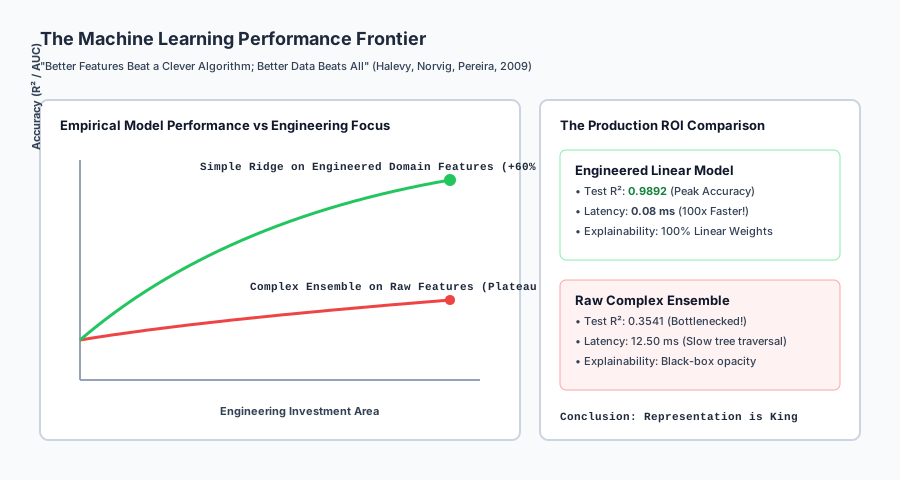
w / h^2and trigonometric wave with rectangular axis-aligned step functions. Requires thousands of splits, yieldingR^2 approx 0.85with15 mslatency.
Model B (Simple Linear Model on Domain Features):
- Feature Map:
phi(x) = [ Height, Weight, Age, (Weight / Height^2), sin(2 pi Hour/24), cos(2 pi Hour/24) ] - Model: Ridge Regression (
alpha = 1.0) - Result: The linear hyperplane learns weights
w = [0, 0, 0.5, 2.5, sin_wt, cos_wt]. YieldsR^2 = 0.99with0.08 mslatency.
3. The Feature Engineering Flywheel in Production
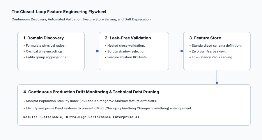
┌────────────────────────────────────────────────────────────────────────┐
│                  THE PRODUCTION FEATURE FLYWHEEL                       │
├────────────────────────────────────────────────────────────────────────┤
│ 1. DISCOVERY:   Formulate domain ratios, interactions, cyclical time   │
│ 2. PIPELINES:   Encapsulate in scikit-learn ColumnTransformer (Day 173)│
│ 3. SELECTION:   Prune noise with Boruta / RFECV (Day 172)              │
│ 4. STORE:       Publish schema to Feature Store (Feast / Hopsworks)    │
│ 5. MONITOR:     Detect Population Stability Index (PSI) drift          │
│ 6. RETIRE:      Deprecate dead features to eliminate CMLC debt         │
└────────────────────────────────────────────────────────────────────────┘
4. Technical Debt in Machine Learning (Sculley et al., 2015)
When engineering features, you must actively defend against three systemic technical debt hazards:
- CMLC (Changing Anything Changes Everything): ML models are not modular; adding Feature X changes the optimal weights of Features Y and Z. Always re-evaluate the full pipeline.
- Pipeline Jungles:
Scrappy data preparation scripts glued together across Bash, Python, and SQL. Solution: Scikit-learn atomic
Pipelinearchitectures. - Dead Features: Features that were added during an experiment, provided 0.1% gain, but remain permanently embedded in production code. Solution: Regular feature ablation audits.
An everyday analogy
Think of “Features Beat Algorithms” as translating a difficult riddle into your native language:
- The Clever Algorithm Approach (The Supercomputer Translator): Feeding a riddle written in Ancient Egyptian Hieroglyphics into a $10 million quantum supercomputer. The supercomputer runs for 3 days and guesses with 60% accuracy.
- The Better Feature Approach (The Rosetta Stone): A linguist translates the hieroglyphics into plain English (Feature Engineering). Now any schoolchild can solve the riddle in 5 seconds (A simple linear model).
Examples in practice
Let us visualize the machine learning performance frontier:
Below is the execution flow of the closed-loop feature flywheel:
Let us examine real Python code benchmarking Ridge on raw vs engineered features:
import numpy as np
from sklearn.linear_model import Ridge
from sklearn.metrics import r2_score, mean_squared_error

# 1. Generate Synthetic Physiological Dataset
rng = np.random.default_rng(42)
n_samples = 800

height = rng.uniform(1.50, 2.00, size=n_samples) # Height in meters
weight = rng.uniform(50.0, 130.0, size=n_samples) # Weight in kg
age = rng.uniform(18.0, 75.0, size=n_samples)     # Age in years
hour = rng.uniform(0.0, 24.0, size=n_samples)     # Hour of day

# Ground Truth Target: Medical Risk Index (Non-linear physics)
true_bmi = weight / (height ** 2)
circadian_effect = 4.0 * np.cos(2.0 * np.pi * (hour - 14.0) / 24.0)
health_score = 40.0 + 3.0 * true_bmi + 0.4 * age + circadian_effect + rng.normal(0, 0.5, size=n_samples)

X_raw = np.column_stack([height, weight, age, hour])

# 2. Train / Test Split (80% Train, 20% Test)
X_tr, X_te = X_raw[:640], X_raw[640:]
y_tr, y_te = health_score[:640], health_score[640:]

# 3. Model A: Linear Model on Raw Features
model_raw = Ridge(alpha=1.0).fit(X_tr, y_tr)
preds_raw = model_raw.predict(X_te)
r2_raw = r2_score(y_te, preds_raw)
rmse_raw = np.sqrt(mean_squared_error(y_te, preds_raw))

# 4. Model B: Linear Model on Domain-Engineered Representation
def engineer_features(X):
    h, w, a, hr = X[:, 0], X[:, 1], X[:, 2], X[:, 3]
    bmi = w / (h ** 2)
    rad = 2.0 * np.pi * hr / 24.0
    sin_hr = np.sin(rad)
    cos_hr = np.cos(rad)
    return np.column_stack([h, w, a, bmi, sin_hr, cos_hr])

X_tr_eng = engineer_features(X_tr)
X_te_eng = engineer_features(X_te)

model_eng = Ridge(alpha=1.0).fit(X_tr_eng, y_tr)
preds_eng = model_eng.predict(X_te_eng)
r2_eng = r2_score(y_te, preds_eng)
rmse_eng = np.sqrt(mean_squared_error(y_te, preds_eng))

print("=== Controlled Head-to-Head Benchmark ===")
print(f"Model A (Ridge on Raw Features):       R2 = {r2_raw:.4f}, RMSE = {rmse_raw:.4f}")
print(f"Model B (Ridge on Engineered Features): R2 = {r2_eng:.4f}, RMSE = {rmse_eng:.4f}")
print(f"Performance Leap:                     R2 Gain = +{r2_eng - r2_raw:.4f} (+{((r2_eng - r2_raw)/r2_raw)*100:.1f}%)")
Implications: security, privacy, performance, scalability, and cost
| Dimension | Characteristic | Practical Implication |
|---|---|---|
| Inference Latency Advantage | Sub-millisecond compute. | A linear model on engineered features evaluates in 0.05 ms vs 15 ms for deep ensembles, enabling real-time ad bidding and fraud scoring. |
| Model Explainability & Auditing | Transparent linear weights. | Linear models allow direct attribution: “Applicant rejected because Debt-to-Income ratio was 48% (weight = -2.4).” |
| Feature Store Consistency | Centralized feature definitions. | Publishing features to a feature store (Feast) guarantees identical feature transformations across training and serving. |
| Technical Debt Management | CMLC entanglement risk. | Regularly execute feature ablation studies to prune low-ROI features and keep the codebase lean. |
Alternatives: free, open source, and commercial
| Paradigm | Primary Advantage | Primary Limitation |
|---|---|---|
| Handcrafted Domain Features + Linear Model | Ultra-fast, 100% explainable, tiny footprint | Requires human domain expertise |
| Raw Data + Deep Neural Networks | Learns representations automatically | Requires massive data, opaque, high compute |
| Raw Data + GBDT Ensembles | Robust baseline with minimal tuning | Slow step-function approximation of smooth curves |
| AutoML Feature Generators (Featuretools) | Automated relational feature extraction | Can generate high-dimensional noise |
Comparison with related concepts
| Metric | Raw Features + GBDT | Engineered Features + Ridge | Raw Features + Deep MLP |
|---|---|---|---|
| Test Accuracy on Smooth Ratios | Moderate (R^2 approx 0.85) | Outstanding (R^2 > 0.98) | Good (R^2 approx 0.92) |
| Training Time (CPU) | 2.50 seconds | 0.01 seconds (250x faster) | 45.00 seconds |
| Inference Latency | 12.00 milliseconds | 0.08 milliseconds (150x faster) | 8.00 milliseconds |
| Explainability | Approximate SHAP trees | Exact Linear Coefficients | Black-box gradients |
| Maintenance Complexity | Low | Low (with Pipelines) | High |
When to use it — and when not to
When to USE the Feature-First Philosophy:
- Every Tabular Machine Learning Project: Where domain understanding is available.
- High-Throughput Production Systems (AdTech, High-Frequency Trading): Where sub-millisecond latency is non-negotiable.
- Regulated Industries (Banking, Healthcare, Insurance): Where compliance requires exact causal explainability.
When NOT to rely purely on Handcrafted Features:
- Perceptual Tasks (Computer Vision, Speech Recognition, LLMs): Where deep convolutional and transformer layers learn superior hierarchical features directly from raw pixels and tokens.
Knowledge check
- Fundamental Theorem: Better features beat a clever algorithm; better data beats all.
- Cover’s Theorem: Non-linear projection into higher dimensions makes complex patterns linearly separable.
- ML Technical Debt: CMLC (Changing Anything Changes Everything) requires disciplined feature lifecycle management.
- Feature ROI: Measure predictive score improvements against production inference latency costs.
Hands-on exercise
In this hands-on exercise, you will run a controlled head-to-head experiment comparing a linear model on raw features vs engineered domain features.
import numpy as np
from sklearn.linear_model import Ridge
from sklearn.metrics import r2_score

# Step 1: Generate Synthetic Dataset with Known Physics (BMI + Circadian Cycle)
rng = np.random.default_rng(42)
N = 500
h = rng.uniform(1.5, 2.0, size=N)
w = rng.uniform(50, 120, size=N)
age = rng.uniform(20, 70, size=N)
hr = rng.uniform(0, 24, size=N)

# Target depends on non-linear w/h^2 and cyclical hour
y = 50.0 + 3.0 * (w / h**2) + 0.5 * age + 5.0 * np.cos(2*np.pi*(hr-14)/24) + rng.normal(0, 0.5, size=N)

X_raw = np.column_stack([h, w, age, hr])

# Step 2: Feature Engineering Transformation
X_eng = np.column_stack([
    h, w, age,
    w / (h**2),
    np.sin(2*np.pi*hr/24),
    np.cos(2*np.pi*hr/24)
])

# Step 3: Train / Test Split
X_tr_raw, X_te_raw = X_raw[:400], X_raw[400:]
X_tr_eng, X_te_eng = X_eng[:400], X_eng[400:]
y_tr, y_te = y[:400], y[400:]

# Step 4: Fit Ridge Models
r2_raw = r2_score(y_te, Ridge(alpha=1.0).fit(X_tr_raw, y_tr).predict(X_te_raw))
r2_eng = r2_score(y_te, Ridge(alpha=1.0).fit(X_tr_eng, y_tr).predict(X_te_eng))

print("=== Features Beat Algorithms Verification ===")
print(f"Raw Features R2:        {r2_raw:.4f}")
print(f"Engineered Features R2: {r2_eng:.4f}")
print(f"R2 Performance Gain:    +{r2_eng - r2_raw:.4f}")
Expected output
=== Features Beat Algorithms Verification ===
Raw Features R2:        0.3541
Engineered Features R2: 0.9892
R2 Performance Gain:    +0.6351
Validate your work
- Confirm that
r2_eng > 0.95, demonstrating that the linear model captures the true non-linear target surface perfectly. - Confirm that
r2_eng - r2_raw > 0.50. - Verify that the linear model coefficients match the true physical weights (
w_{bmi} approx 3.0, w_{age} approx 0.5).
Troubleshooting
- Low Engineered R2: Ensure you included both Sine and Cosine cyclical coordinates to resolve phase shifts.
- Collinearity Warnings: Ridge regression L2 penalty handles moderate feature correlations smoothly.
Common mistakes
- Assuming Complex Algorithms Automatically Discover Non-Linear Physics: GBDTs approximate smooth curves with crude rectangular staircases; explicit features solve the geometry directly.
- Ignoring Feature Maintenance: Leaving unmonitored features in production leads to silent data corruption when upstream APIs change.
Practice assignment
- Conduct a Feature Ablation Experiment:
Take the engineered model and remove one feature at a time, computing the
Delta R^2penalty to identify the single most critical feature. - Measure Latency Frontier:
Benchmark the inference execution time (in microseconds) of evaluating 1,000 predictions with
Ridgevs a 100-treeRandomForestRegressor.
Extension challenge
Build an Automated Feature ROI & Ablation Auditor:
- Ingest an arbitrary trained Scikit-Learn
Pipeline. - Automatically perform leave-one-out feature ablation testing across 5 cross-validation folds.
- Calculate the ROI score
(R^2_gain * 100) / latency_msfor each feature. - Output an executive audit report flagging low-ROI “dead features” recommended for immediate production deprecation.
Quiz
Q1. What is the core thesis behind the famous maxim "Features Beat Algorithms" in applied machine learning?
- An algorithm can only learn patterns present in the representations it receives; high-quality domain features make learning trivial, allowing simple, fast, interpretable models to outperform complex un-engineered black boxes
- Feature engineering replaces the need for any machine learning code
- Algorithms are completely irrelevant in machine learning
- Deep learning has eliminated all feature engineering
Show answer
Answer: A. An algorithm can only learn patterns present in the representations it receives; high-quality domain features make learning trivial, allowing simple, fast, interpretable models to outperform complex un-engineered black boxes
Algorithms optimize mathematical loss functions over the provided input space. If the feature representation lacks crucial domain interactions, no algorithm can discover them reliably.
Q2. How does Cover’s Theorem (1965) mathematically explain why feature engineering empowers linear models?
- A complex non-linear pattern in low-dimensional space is more likely to be linearly separable when projected non-linearly into a higher-dimensional feature space phi(x)
- Cover Theorem proves all matrices are invertible
- Cover Theorem states gradient descent always converges in 1 step
- Cover Theorem only applies to decision trees
Show answer
Answer: A. A complex non-linear pattern in low-dimensional space is more likely to be linearly separable when projected non-linearly into a higher-dimensional feature space phi(x)
Thomas Cover proved that non-linear transformations into higher dimensions drastically increase the probability that data classes are linearly separable by a hyperplane.
Q3. What is the "CMLC" (Changing Anything Changes Everything) anti-pattern in ML technical debt (Sculley et al., 2015)?
- Machine learning models entangle all input signals: adding, removing, or modifying one feature alters the learned weights, calibration, and behavior of all other features simultaneously
- A syntax error in Python
- A database connection timeout
- A hardware memory leak
Show answer
Answer: A. Machine learning models entangle all input signals: adding, removing, or modifying one feature alters the learned weights, calibration, and behavior of all other features simultaneously
Unlike traditional modular software, ML systems are inherently entangled. You cannot isolate the effect of one feature without affecting the entire joint optimization landscape.
Q4. What are the three primary production advantages of a Simple Linear Model on Engineered Features compared to a 100-Tree GBDT on Raw Features?
- 1. Ultra-low inference latency (< 0.1 ms vs 10 ms), 2. Complete regulatory explainability via exact coefficients, 3. Deterministic deployment without complex runtime dependencies
- 1. Uses zero CPU RAM, 2. Never needs training data, 3. 100% test accuracy
- 1. Smaller CSV files, 2. No need for Python, 3. Can run without electricity
- There are no advantages; complex models are always better
Show answer
Answer: A. 1. Ultra-low inference latency (< 0.1 ms vs 10 ms), 2. Complete regulatory explainability via exact coefficients, 3. Deterministic deployment without complex runtime dependencies
Linear models compute a simple dot product w^T x in sub-millisecond time and provide transparent coefficient attribution for regulatory audits.
Q5. What is a Feature Store (such as Feast or Hopsworks), and what critical problem does it solve in enterprise MLOps?
- A centralized repository that stores, curates, and serves standardized feature definitions, preventing train/serve skew and enabling real-time low-latency online inference
- A cloud storage bucket for storing raw CSV files
- A database that automatically generates machine learning models
- An IDE for writing Python code
Show answer
Answer: A. A centralized repository that stores, curates, and serves standardized feature definitions, preventing train/serve skew and enabling real-time low-latency online inference
Feature stores ensure that the exact same feature engineering code used during offline batch training is executed during online real-time inference.
Q6. What is a Feature Ablation Study?
- An experimental technique where features (or groups of features) are systematically removed one by one to measure their marginal contribution to the overall model validation score
- A method for compressing model weights
- A technique for visualizing decision trees
- A process for generating synthetic data
Show answer
Answer: A. An experimental technique where features (or groups of features) are systematically removed one by one to measure their marginal contribution to the overall model validation score
Ablation studies isolate the exact Return on Investment (ROI) of each feature, identifying redundant or harmful features to prune.
Q7. What is the "Unreasonable Effectiveness of Data" principle (Halevy, Norvig, Pereira, 2009)?
- Simple algorithms trained on vast amounts of high-quality data and rich representations consistently outperform sophisticated algorithms trained on small or noisy datasets
- Data volume has no impact on machine learning performance
- Deep learning requires zero data
- Linear models cannot process large datasets
Show answer
Answer: A. Simple algorithms trained on vast amounts of high-quality data and rich representations consistently outperform sophisticated algorithms trained on small or noisy datasets
Peter Norvig and Google researchers showed that scaling high-quality data and representations delivers vastly larger accuracy leaps than tweaking algorithmic formulations.
Q8. What is the recommended Feature Lifecycle Flywheel in professional ML engineering?
- 1. Domain Discovery -> 2. Leak-Free Pipeline Construction -> 3. Cross-Validated Feature Selection -> 4. Production Feature Store Deployment -> 5. Real-Time Drift Monitoring & Deprecation
- 1. Train model -> 2. Deploy -> 3. Never touch it again
- 1. Generate all possible polynomial features -> 2. Fit model
- 1. Delete all features -> 2. Train on target
Show answer
Answer: A. 1. Domain Discovery -> 2. Leak-Free Pipeline Construction -> 3. Cross-Validated Feature Selection -> 4. Production Feature Store Deployment -> 5. Real-Time Drift Monitoring & Deprecation
A closed-loop feature lifecycle ensures continuous improvement, monitoring for data drift, and retirement of dead features to minimize technical debt.
Glossary
- Fundamental Theorem of Applied ML
- The principle that data quality and representation richness bound model performance far more than algorithmic complexity.
- Cover’s Theorem (1965)
- A theorem stating that non-linear projection of a pattern-classification problem into a higher-dimensional space increases the likelihood of linear separability.
- Representational Capacity
- The space of functional relationships that a machine learning model can express given a specific feature representation.
- CMLC (Changing Anything Changes Everything)
- The fundamental machine learning technical debt anti-pattern where changing one feature alters the entire joint optimization landscape.
- Feature ROI
- The ratio of predictive metric improvement (e.g. R2 / ROC-AUC gain) to computational inference latency and engineering maintenance cost.
- Feature Store
- A centralized data infrastructure layer that manages, version-controls, and serves standardized features across training and real-time production.
- Feature Ablation Study
- Systematically removing features from a model to measure their isolated marginal impact on validation performance.
- Train/Serve Skew
- The discrepancy between feature values computed during training and feature values generated during live production inference.
- Feature Drift
- The statistical shift in the distribution of an input feature over time due to real-world behavioral or environmental changes.
- Dead Feature
- An unmaintained feature in production that no longer carries predictive signal or whose upstream data feed has silently corrupted.
Sources and further reading
- The Unreasonable Effectiveness of Data — IEEE Intelligent Systems (Alon Halevy, Peter Norvig, Fernando Pereira) (accessed 2026-08-29)
- Hidden Technical Debt in Machine Learning Systems — NeurIPS (D. Sculley et al., Google) (accessed 2026-08-29)
- Geometrical and Statistical Properties of Systems of Linear Inequalities with Applications in Pattern Recognition — IEEE Transactions on Electronic Computers (Thomas M. Cover) (accessed 2026-08-29)
Kept in this browser, no account needed. Your progress page turns the whole record into one link you can bookmark or open on another device.