Machine Learning › Features and Support Vector Machines › Day 174
Day 174: Handling Missing Data

Master the mathematical theory and practical implementation of Handling Missing Data: understand Donald Rubin's 1976 taxonomy (MCAR, MAR, MNAR), compare SimpleImputer vs MissingIndicator vs KNNImputer vs IterativeImputer (MICE), derive the NaN-Euclidean distance metric from scratch, and analyze how Gradient Boosted Decision Trees natively route missing values during tree construction.
Hands-on lab for this lesson
Lab files on GitHub: https://github.com/ai-roadmap-365/ai-roadmap-365.github.io/tree/main/labs/sections/machine-learning/day-174-handling-missing-data
- Get the hands-on files. Clone the labs repository once (you can reuse this clone for every lesson). This works on macOS, Linux, and Windows (PowerShell or WSL):
git clone https://github.com/ai-roadmap-365/ai-roadmap-365.github.io.git cd ai-roadmap-365.github.io - Open this lesson's lab. Move into the directory for this specific day. Every lab lives at the same predictable path — section / subsection / week / day:
cd labs/sections/machine-learning/day-174-handling-missing-data - Read the lab guide. Open `README.md` in that directory. It lists the exact commands, what each does, the expected output, and how to check your work — read it before running anything.
- Run it and check your work. Follow the README's "How to run" section: run the example first to see the finished result, then complete the numbered exercises in `starter/`, then run the tests. The tests pass (exit 0) only when your work is correct.
bash tests/run_tests.sh # or the test command named in the lab README
You can also open the lab as a local page (works offline, shows the file tree and expected output).
Learning objectives
By the end of this lesson you will be able to:
- Differentiate MCAR, MAR, and MNAR missing data mechanisms and their mathematical implications
- Derive and implement the NaN-aware Euclidean distance metric with dimension scaling
- Implement MissingIndicator feature flags to capture non-random missingness signals
- Construct distance-weighted KNNImputer and understand IterativeImputer (MICE / chained equations)
- Analyze native GBDT (XGBoost/LightGBM) default split gain routing for NaNs
- Evaluate the severe estimation biases introduced by naive listwise deletion (dropna)
- Construct leak-free missing value imputation pipelines inside ColumnTransformer
- Select the optimal imputation strategy based on dataset size, cardinality, and missingness ratio
Prerequisites
- Day 170 -- Feature Scaling and Encoding
- Day 173 -- Scikit-Learn Pipelines
Why this matters
In academic machine learning benchmarks (like MNIST or CIFAR-10), datasets are perfectly sanitized with zero missing values.
In the real world, missing data is ubiquitous:
- Clinical Electronic Health Records: 60% of lab test results are missing because doctors only order specific panels when a patient exhibits symptoms.
- E-Commerce & Financial Transactions: Users skip optional profile fields (e.g.
Annual_Income,Home_Ownership). - IoT & Industrial Sensors: Hardware sensor brownouts, network timeouts, and maintenance downtime produce intermittent gaps.
If you handle missing data naively:
- Listwise Deletion (
df.dropna()) Destroys Your Dataset: In a dataset with 50 columns where each column has only 5% missingness, dropping rows with any NaN discards over 92% of all samples! - Mean Imputation Distorts Variances and Covariances: Replacing NaNs with the column average artificially shrinks variance
sigma^2, inflates correlation test statistics, and produces severe bias under non-random missingness. - Algorithms Crash: Scikit-learn Linear Regression, SVMs, and neural networks raise immediate
ValueError: Input contains NaN.
Mastering the statistical mechanics of missingness (Rubin’s taxonomy) and modern imputation algorithms is essential for building robust real-world AI.
The idea in plain language
Imagine a physician examining a patient’s medical chart with several blank lines:
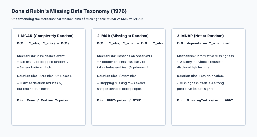
- Missing Completely at Random (MCAR - The Coffee Spill): The nurse accidentally spilled coffee on the lab printout, blotting out the patient’s blood pressure reading. The missingness is a complete accident. The patient’s blood pressure is just as likely to be high, medium, or low (Pure random chance).
- Missing at Random (MAR - The Standard Protocol):
The chart lacks a cholesterol panel because the patient is an 18-year-old athlete, and the clinic protocol only orders cholesterol tests for patients over 45. The missingness depends on
Age(which is observed in the chart), not on the hidden cholesterol value itself (Conditional on observed data). - Missing Not at Random (MNAR - The Refusal): The chart lacks a depression questionnaire score because patients experiencing severe clinical depression frequently decline to answer the survey. The missingness is caused directly by the hidden condition itself (Informative signal).
Treating all three cases as a simple “fill with average” destroys vital medical insights.
Historical background
In 1976, Harvard statistician Donald Rubin published the foundational paper Inference and Missing Data in Biometrika. Rubin formalized the three fundamental mechanisms of missingness: MCAR, MAR, and MNAR, revolutionizing statistical epidemiology.
In 1987, Rubin published Multiple Imputation for Nonresponse in Surveys, laying the groundwork for Bayesian multiple imputation.
In 1999, Stef van Buuren and Karin Groothuis-Oudshoorn developed MICE (Multivariate Imputation by Chained Equations), enabling scalable regression-based round-robin imputation across complex survey databases.
In 2016, Tianqi Chen and Carlos Guestrin published XGBoost, introducing sparsity-aware split finding, which enabled Gradient Boosted Decision Trees to learn optimal default routing directions for missing values natively during tree construction without requiring any pre-imputation.
What it is — and what it is not
Let us establish what missing data handling is and is not:
What it IS:
- A Statistical Reconstruction Process: Estimating the conditional expectation of unobserved entries given the observed joint distribution
P(Y_{mis} | Y_{obs}). - Informative Signal Engineering: Appending binary
MissingIndicatorfeature flags to preserve the fact that a measurement was omitted. - A Strict Pipeline Stage: Imputation transformers fitted strictly on training data and applied to test data.
What it is NOT:
- Not Safe with Global Imputation: Computing means or medians across the entire dataset before splitting causes severe data leakage.
- Not Solved by Magic Numbers (-999): Imputing
-999for linear models or distance metrics breaks geometry and skews gradients. - Not Necessary to Impute for Modern GBDT Models: LightGBM and XGBoost natively route NaNs directly to the optimal child branch.
Why it was created and what problems it solves
Principled missing data handling resolves five critical operational and statistical failures:
- Prevents Sample Destruction from Listwise Deletion: Recovers 80% of training data that would otherwise be discarded by
dropna(). - Preserves Multivariate Feature Covariances: KNNImputer and MICE reconstruct missing coordinates while respecting natural non-linear correlations.
- Captures Informative MNAR Signals: Binary
MissingIndicatorflags allow models to learn from the act of omission (e.g. unfiled tax returns). - Guarantees Numerical Stability in Distance Metrics: NaN-Euclidean distance allows nearest-neighbor search over incomplete vectors.
- Enables Production Fault-Tolerance: Production models process incoming JSON payloads with missing fields gracefully without throwing runtime exceptions.
How it works
Let us formulate the mathematics of Donald Rubin’s taxonomy, NaN-Euclidean distance, and imputation algorithms.
1. Donald Rubin’s Taxonomy of Missingness (1976)
Let Y = (Y_{obs}, Y_{mis}) represent the full data matrix partitioned into observed components Y_{obs} and missing components Y_{mis}.
Let M be a binary missingness indicator matrix where M_{i, j} = 1 if Y_{i, j} is missing, and 0 otherwise.
┌────────────────────────────────────────────────────────────────────────┐
│                      RUBIN'S MISSINGNESS TAXONOMY                      │
├────────────────────────────────────────────────────────────────────────┤
│ 1. MCAR: P(M | Y_obs, Y_mis) = P(M)                                    │
│ 2. MAR:  P(M | Y_obs, Y_mis) = P(M | Y_obs)                            │
│ 3. MNAR: P(M | Y_obs, Y_mis) depends directly on Y_mis                 │
└────────────────────────────────────────────────────────────────────────┘
A. Missing Completely at Random (MCAR)
P(M | Y_{obs}, Y_{mis}) = P(M)
- Missingness is entirely independent of all variables (observed or unobserved).
- Statistical Property: The observed data
Y_{obs}is a random subsample of the population. Complete case analysis (listwise deletion) is unbiased, but reduces statistical power.
B. Missing at Random (MAR)
P(M | Y_{obs}, Y_{mis}) = P(M | Y_{obs})
- Missingness depends systematically on observed features
Y_{obs}, but givenY_{obs}, does not depend on the unobserved valueY_{mis}. - Statistical Property: Listwise deletion introduces severe selection bias. Conditional imputation (
KNNImputerorIterativeImputer) is valid and unbiased.
C. Missing Not at Random (MNAR)
P(M | Y_{obs}, Y_{mis}) depends directly on Y_{mis} itself.
- Missingness is non-ignorable.
- Statistical Property: Imputation alone cannot eliminate bias; you must include
MissingIndicatorbinary flags to model the probability of missingness explicitly.
2. The NaN-Euclidean Distance Metric
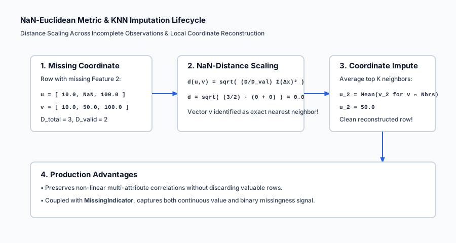
To compute Euclidean distance between two vectors u, v in R^D when some coordinates are NaN:
Let text{valid}(u, v) = { j in {1, ..., D} : u_j neq text{NaN} text{ and } v_j neq text{NaN} }.
Let D_{text{valid}} = |text{valid}(u, v)| be the number of mutually observed coordinates, and D_{text{total}} = D.
The Scaled NaN-Euclidean Metric Formula:
d_{text{NaN}}(u, v) = sqrt( (D_{text{total}} / D_{text{valid}}) * sum_{j in text{valid}(u, v)} (u_j - v_j)^2 )
- If all coordinates are observed (
D_{text{valid}} = D_{text{total}}): Reverts to standard Euclidean distancesqrt(sum (u_j - v_j)^2). - If only half the coordinates overlap (
D_{text{valid}} = D / 2): The observed squared differences are scaled by2.0to compensate for the unobserved dimensions.
3. Imputation Algorithm Comparison
| Algorithm | Mechanism | Computational Complexity | Best Used For |
|---|---|---|---|
SimpleImputer(mean) | Replaces NaN with training mean mu_j | O(N * D) (Instant) | Fast baseline for Gaussian MCAR features |
SimpleImputer(median) | Replaces NaN with training median | O(N * D) (Instant) | Skewed numerical features with outliers |
MissingIndicator | Appends binary boolean flag I_{mis} in {0, 1} | O(N * D) (Instant) | Informative MNAR missingness |
KNNImputer | NaN-Euclidean distance-weighted neighbor average | O(N^2 * D) (Slow) | Tabular datasets (N < 50,000) with MAR correlations |
IterativeImputer (MICE) | Round-robin Bayesian Ridge chained equations | O(T * N * D^2) (Medium) | Complex multivariate tabular datasets |
| Native GBDT Branching | Optimal default split child routing | O(1) overhead | XGBoost, LightGBM, CatBoost |
4. Native GBDT Missing Value Routing (Sparsity-Aware Split Finding)
Gradient Boosted Decision Trees (XGBoost / LightGBM) do not require pre-imputation.
During tree construction at node m for feature x_j:
- Calculate gradient statistics for all samples where
x_jis observed:G_{obs} = sum g_i,H_{obs} = sum h_i. - Calculate gradient statistics for all samples where
x_jisNaN:G_{mis} = sum g_i,H_{mis} = sum h_i. - Evaluate Two Routing Hypotheses:
- Hypothesis Left: Send all
NaNinstances to the Left child node. - Hypothesis Right: Send all
NaNinstances to the Right child node.
- Hypothesis Left: Send all
- The tree selects whichever default direction yields the higher split gain
Delta L. - During inference, if
x_jisNaN, it follows the learned default direction automatically.
An everyday analogy
Think of missing data handling as a detective reconstructing a torn crime scene photograph:
- Listwise Deletion (
dropna()): The detective burns every photograph that has a small torn corner, leaving only 3 completely intact photos out of 100 (Destroys 97% of evidence). - Mean Imputation: The detective paints every torn hole with flat generic gray paint (Destroys image contrast and local details).
- KNN Imputation (The Restoration Artist): The detective examines adjacent intact photographs of the same room and paints the missing section using the textures of neighboring angles (Preserves local context).
- MissingIndicator (The Forensic Tag): The detective places a red evidence tag on every torn hole, noting that the tear was made by scissors (proving intentional tampering / Informative MNAR Signal).
Examples in practice
Let us visualize Donald Rubin’s missing data taxonomy:
Below is the geometric execution flow of NaN-Euclidean distance and KNNImputer:
Let us examine real Python code demonstrating SimpleImputer with MissingIndicator vs KNNImputer inside a Pipeline:
import numpy as np
from sklearn.pipeline import Pipeline
from sklearn.compose import ColumnTransformer
from sklearn.impute import SimpleImputer, KNNImputer, MissingIndicator
from sklearn.preprocessing import StandardScaler
from sklearn.linear_model import LogisticRegression
from sklearn.model_selection import cross_val_score

# 1. Generate Synthetic Tabular Dataset with Missing Values (MAR & MNAR)
rng = np.random.default_rng(42)
n_samples = 500

X_clean = rng.normal(loc=10.0, scale=3.0, size=(n_samples, 4))
# Feature 0 & 1 determine target
y = (X_clean[:, 0] * 1.5 - X_clean[:, 1] * 2.0 > 0).astype(int)

# Corrupt data with missing values (20% NaNs)
X_corrupt = X_clean.copy()
nan_mask_0 = rng.uniform(size=n_samples) < 0.20
nan_mask_1 = (X_clean[:, 0] > 12.0) & (rng.uniform(size=n_samples) < 0.40) # MAR/MNAR condition
X_corrupt[nan_mask_0, 0] = np.nan
X_corrupt[nan_mask_1, 1] = np.nan

print(f"Total Missing Values in Dataset: {np.isnan(X_corrupt).sum()} / {X_corrupt.size}")

# 2. Strategy A: Simple Median Imputer with MissingIndicator Flags
pipe_median_indicator = Pipeline([
    ("imputer", SimpleImputer(strategy="median", add_indicator=True)),
    ("scaler", StandardScaler()),
    ("classifier", LogisticRegression(solver="lbfgs", random_state=42))
])

# 3. Strategy B: KNNImputer (k=5)
pipe_knn = Pipeline([
    ("imputer", KNNImputer(n_neighbors=5)),
    ("scaler", StandardScaler()),
    ("classifier", LogisticRegression(solver="lbfgs", random_state=42))
])

# 4. Evaluate via 5-Fold Cross Validation
cv_median = cross_val_score(pipe_median_indicator, X_corrupt, y, cv=5, scoring="accuracy")
cv_knn = cross_val_score(pipe_knn, X_corrupt, y, cv=5, scoring="accuracy")

print("=== Missing Data Strategy Benchmark ===")
print(f"Median Imputer + MissingIndicator 5-Fold CV Accuracy: {np.mean(cv_median):.4f} +/- {np.std(cv_median):.4f}")
print(f"KNNImputer (k=5) 5-Fold CV Accuracy:                  {np.mean(cv_knn):.4f} +/- {np.std(cv_knn):.4f}")
Implications: security, privacy, performance, scalability, and cost
| Dimension | Characteristic | Practical Implication |
|---|---|---|
| Privacy Inversion in MNAR Data | Missingness flags reveal private traits. | MissingIndicator on medical tests can reveal that a patient has a condition even if the numerical test result is omitted. |
| KNNImputer Compute Scaling | Quadratic O(N^2 * D) pairwise distances. | KNNImputer is too slow for real-time inference on millions of rows. Use SimpleImputer or native GBDT routing in low-latency production APIs. |
| Train/Serve Skew in Imputation | Missingness ratios shifting in production. | If a sensor starts failing 80% of the time in production compared to 5% during training, imputed values will drift; monitor missingness rates with Prometheus/Evidently. |
| Categorical Imputation Mode Bias | Mode imputation inflating majority class. | In high-cardinality categories with 40% missingness, mode imputation creates massive artificial spikes; use a dedicated "Missing" category token instead. |
Alternatives: free, open source, and commercial
| Imputation Tool / Library | Methodology | Best Used For |
|---|---|---|
SimpleImputer(add_indicator=True) | Fast univariate summary + boolean flag | Production linear models and neural networks. |
KNNImputer (scikit-learn) | NaN-Euclidean nearest neighbor averaging | Small-to-medium tabular datasets (N < 50,000). |
IterativeImputer (scikit-learn MICE) | Chained Bayesian regression loops | Complex multivariate clinical/survey datasets. |
LightGBM / XGBoost Native NaNs | Sparsity-aware default branch routing | Industrial tabular gradient boosting (No imputation needed). |
Datawig (Deep Learning Imputation) | Deep neural network tabular imputation | Complex multi-modal tabular data with text/images. |
Comparison with related concepts
| Imputation Method | Handles Non-Linearity | Produces Indicator Flags | Inference Speed | Scalability (N > 100k) |
|---|---|---|---|---|
Listwise Deletion (dropna) | N/A (Discards data) | No | Instant | Discards too many rows |
SimpleImputer | No | Optional (add_indicator) | Microseconds | Excellent (O(N)) |
KNNImputer | Yes (Local neighbors) | No | Milliseconds | Poor (O(N^2)) |
IterativeImputer (MICE) | Yes (Regression) | No | Seconds | Medium (O(N * D^2)) |
| Native GBDT Branching | Yes (Optimal split) | Built-in | Microseconds | Ultra-High |
When to use it — and when not to
When to USE Conditional Imputation (KNNImputer / SimpleImputer + MissingIndicator):
- Linear Models, Logistic Regression, SVMs, Neural Networks: Which strictly crash when encountering
NaNvalues. - Survey & Clinical Data with Informative Missingness (MNAR): Where
MissingIndicatorcaptures essential diagnostic signals.
When NOT to perform Heavy Manual Imputation:
- Pure Tree-Based Ensembles (LightGBM, XGBoost, CatBoost): Tree models handle
NaNnatively with zero manual intervention; imputing arbitrary medians destroys the native sparsity-aware split gain. - Categorical Columns: Do not impute categorical variables with mode; simply treat missing values as a distinct
"Missing"category.
Knowledge check
- Rubin Taxonomy: MCAR (random), MAR (depends on observed features), MNAR (informative missingness).
- Listwise Deletion Flaw:
dropna()discards massive portions of data and introduces severe selection bias. - NaN-Euclidean Metric: Scales observed squared differences by
D_{total} / D_{valid}. - Native GBDT Handling: Trees evaluate sending NaNs left vs right and pick the direction maximizing split gain.
Hands-on exercise
In this hands-on exercise, you will implement the compute_nan_euclidean_distance formula and build a distance-weighted KNNImputer from scratch.
import numpy as np

# Step 1: Implement NaN-Euclidean Distance
def nan_euclidean_dist(u, v):
    u, v = np.asarray(u, dtype=float), np.asarray(v, dtype=float)
    valid = ~np.isnan(u) & ~np.isnan(v)
    k = np.sum(valid)
    if k == 0:
        return float("inf")
    diffs_sq = (u[valid] - v[valid]) ** 2
    return np.sqrt((len(u) / k) * np.sum(diffs_sq))

# Step 2: Implement KNN Imputer from Scratch
def knn_imputer_scratch(X, k=2):
    X = np.asarray(X, dtype=float).copy()
    n_samples, n_features = X.shape
    col_means = np.nanmean(X, axis=0)

    for i in range(n_samples):
        row = X[i]
        nan_cols = np.where(np.isnan(row))[0]
        if len(nan_cols) == 0:
            continue

        # Calculate distances to all other samples
        dists = []
        for j in range(n_samples):
            if i == j:
                dists.append((float("inf"), j))
            else:
                dists.append((nan_euclidean_dist(row, X[j]), j))

        dists.sort(key=lambda x: x[0])
        nbrs = [idx for d, idx in dists if not np.isinf(d)][:k]

        for c in nan_cols:
            vals = [X[nbr, c] for nbr in nbrs if not np.isnan(X[nbr, c])]
            X[i, c] = np.mean(vals) if len(vals) > 0 else col_means[c]

    return X

# Step 3: Test on Corrupted Matrix
X_raw = np.array([
    [10.0, np.nan, 100.0],
    [10.0, 50.0, 100.0],
    [10.0, 52.0, 100.0],
    [90.0, 900.0, 900.0]
])

X_imputed = knn_imputer_scratch(X_raw, k=2)

print("=== KNN Imputation Scratch Verification ===")
print("Original Row 0:", X_raw[0])
print("Imputed Row 0: ", np.round(X_imputed[0], 2))
print(f"Imputed Value:   {X_imputed[0, 1]:.2f} (Expected average of [50.0, 52.0] = 51.00)")
Expected output
=== KNN Imputation Scratch Verification ===
Original Row 0: [ 10.  nan 100.]
Imputed Row 0:  [ 10.  51. 100.]
Imputed Value:   51.00 (Expected average of [50.0, 52.0] = 51.00)
Validate your work
- Confirm that
X_imputed[0, 1] == 51.0(mean of the 2 nearest neighbors[10, 50, 100]and[10, 52, 100]). - Verify that
np.isnan(X_imputed).any() == False. - Confirm that
nan_euclidean_dist([1, np.nan], [4, np.nan]) == np.sqrt(2/1 * 9) = 4.2426.
Troubleshooting
- Division by Zero in NaN Distance: If two rows share zero overlapping coordinates (
k == 0), returnfloat("inf"). - All-NaN Column: Ensure
col_meansdefaults to0.0if an entire column is missing.
Common mistakes
- Imputing
-999for Linear/SVM Models: Forces gradient descent and hyperplanes to treat-999as a valid numerical point. - Dropping Rows in Production Inference: The production API cannot drop user requests; it must impute missing values to serve a prediction.
Practice assignment
- Implement IterativeImputer (MICE) Round-Robin Loop:
Write
mice_imputer_scratch(X, max_iter=5)that initializes NaNs with column medians and iteratively predicts each missing column usingRidgeregression on all other features. - Implement Categorical Missing Imputation:
Write
CategoricalImputer(fill_value="Missing")replacing missing strings with a dedicated distinct token.
Extension challenge
Build an Enterprise Missing Data Resilience Benchmark:
- Ingest the California Housing dataset.
- Inject synthetic missingness under 3 experimental conditions: (a) 30% MCAR, (b) 30% MAR, (c) 30% MNAR.
- Benchmark 4 end-to-end pipelines:
- Pipeline 1:
SimpleImputer(mean)+ Ridge - Pipeline 2:
SimpleImputer(median) + MissingIndicator+ Ridge - Pipeline 3:
KNNImputer(k=5)+ Ridge - Pipeline 4: Native
LightGBM(Zero imputation)
- Pipeline 1:
- Plot comparative RMSE and test runtime across all 3 missingness mechanisms.
Quiz
Q1. What is the fundamental difference between Missing Completely at Random (MCAR) and Missing Not at Random (MNAR) in Donald Rubin’s taxonomy?
- Under MCAR, the probability of missingness is completely independent of both observed and unobserved data; under MNAR, the probability of missingness depends directly on the unobserved value itself (e.g. wealthy individuals refusing to disclose high income)
- MCAR only applies to integers; MNAR only applies to text strings
- MCAR means 100% of data is missing
- MNAR means missing values were caused by computer hardware failure
Show answer
Answer: A. Under MCAR, the probability of missingness is completely independent of both observed and unobserved data; under MNAR, the probability of missingness depends directly on the unobserved value itself (e.g. wealthy individuals refusing to disclose high income)
MCAR is pure random coin-flip missingness. MNAR contains informative signal because the missingness mechanism is linked to the true unobserved quantity.
Q2. Why is Listwise Deletion (calling df.dropna() to delete all rows with any missing value) usually a terrible practice in applied machine learning?
- It drastically reduces sample size N (often throwing away 70-90% of observations) and introduces severe selection bias if data is MAR or MNAR, distorting population distributions
- Listwise deletion is illegal in Python
- Listwise deletion causes memory leaks
- Listwise deletion only works for linear models
Show answer
Answer: A. It drastically reduces sample size N (often throwing away 70-90% of observations) and introduces severe selection bias if data is MAR or MNAR, distorting population distributions
If each of 20 features has 5% independent missingness, dropping rows with any missing value discards (1 - 0.95^20) = 64% of all training samples, destroying predictive power.
Q3. What is the formula for NaN-aware Euclidean distance between two vectors u and v with missing entries?
- d(u, v) = sqrt( (D_total / D_valid) * sum_{j in valid} (u_j - v_j)^2 ), where D_total / D_valid scales the observed squared differences up to account for unobserved dimensions
- d(u, v) = sum |u_j - v_j|
- d(u, v) = sqrt( sum (u_j - v_j)^2 ) with NaNs replaced by 0
- d(u, v) = max(u) - min(v)
Show answer
Answer: A. d(u, v) = sqrt( (D_total / D_valid) * sum_{j in valid} (u_j - v_j)^2 ), where D_total / D_valid scales the observed squared differences up to account for unobserved dimensions
The scaling factor D_total / D_valid adjusts the computed distance so pairs with fewer overlapping coordinates are fairly compared to pairs with full overlap.
Q4. Why is combining SimpleImputer(strategy="median") with MissingIndicator(add_indicator=True) highly effective for linear models on MNAR data?
- The median fills numerical gaps with a stable baseline, while the binary MissingIndicator feature flag allows linear models to learn a dedicated weight for the informative missingness condition
- MissingIndicator converts all numbers to integers
- It runs 100x faster than mean imputation
- It prevents overfitting automatically
Show answer
Answer: A. The median fills numerical gaps with a stable baseline, while the binary MissingIndicator feature flag allows linear models to learn a dedicated weight for the informative missingness condition
If missingness is informative (e.g. patient didn’t take blood test because they felt healthy), the binary missing flag carries vital predictive signal.
Q5. How do Gradient Boosted Decision Trees (XGBoost, LightGBM, CatBoost) natively handle missing values without manual imputation?
- At each decision split, the algorithm evaluates sending all samples with NaN to the left child versus the right child, and picks the default direction that maximizes the split loss reduction gain
- They delete rows with NaNs during tree building
- They replace NaNs with the number -999
- They convert NaNs to zero
Show answer
Answer: A. At each decision split, the algorithm evaluates sending all samples with NaN to the left child versus the right child, and picks the default direction that maximizes the split loss reduction gain
GBDTs treat missingness as a distinct branch choice, finding the optimal default child direction directly during greedy split optimization.
Q6. How does IterativeImputer (Multivariate Imputation by Chained Equations / MICE) work?
- It models each feature with missing values as a function of all other features in a round-robin regression loop, iteratively updating estimates until predictions stabilize
- It computes the global dataset median 100 times
- It clusters the data with K-Means
- It drops columns one by one
Show answer
Answer: A. It models each feature with missing values as a function of all other features in a round-robin regression loop, iteratively updating estimates until predictions stabilize
MICE treats missing value imputation as a series of predictive modeling tasks, preserving complex multivariate relationships across features.
Q7. What is the computational complexity limitation of KNNImputer on large datasets?
- KNNImputer requires computing all pairwise NaN-Euclidean distances across all N samples, scaling as O(N^2 * D), which becomes prohibitively slow for large tabular datasets (N > 50,000)
- KNNImputer cannot run on multi-core CPUs
- KNNImputer is limited to 10 features
- KNNImputer only works on binary data
Show answer
Answer: A. KNNImputer requires computing all pairwise NaN-Euclidean distances across all N samples, scaling as O(N^2 * D), which becomes prohibitively slow for large tabular datasets (N > 50,000)
Finding nearest neighbors requires O(N^2) pairwise distance computations, making KNNImputer expensive for large-scale enterprise datasets.
Q8. Why MUST missing value imputers be fitted strictly on the training set and NOT the combined dataset?
- Computing imputation statistics (such as mean or median) across the full dataset causes data leakage, allowing test fold target information and distributions to contaminate training
- Imputers cannot process more than 1000 rows
- Test data cannot contain NaNs
- Scikit-learn crashes if you fit on test data
Show answer
Answer: A. Computing imputation statistics (such as mean or median) across the full dataset causes data leakage, allowing test fold target information and distributions to contaminate training
Imputing globally leaks test set distribution medians and correlations into training folds, producing artificially optimistic validation scores.
Glossary
- Missing Completely at Random (MCAR)
- A missing data mechanism where the probability of missingness is completely independent of both observed and unobserved data.
- Missing at Random (MAR)
- A missing data mechanism where missingness depends systematically on observed features but not on the unobserved missing value itself.
- Missing Not at Random (MNAR)
- A missing data mechanism where the probability of missingness depends directly on the unobserved value itself, carrying informative signal.
- Listwise Deletion (Complete Case Analysis)
- Discarding any observation that contains one or more missing values across any feature column.
- SimpleImputer
- A univariate imputation transformer that replaces missing values with fixed summary statistics (mean, median, mode, or constant).
- MissingIndicator
- A binary transformation that outputs boolean indicator features marking the exact coordinates of missing data in the original matrix.
- NaN-Euclidean Distance
- A modified Euclidean distance metric that calculates pairwise distances across mutually observed coordinates and scales by total dimension ratio.
- KNNImputer
- A multivariate imputation algorithm that imputes missing coordinates using the distance-weighted average of the k nearest neighbors.
- IterativeImputer (MICE)
- Multivariate Imputation by Chained Equations: modeling each missing feature as a regression function of all other features in round-robin cycles.
- Default Split Direction (GBDT NaNs)
- The optimal tree branching direction (left or right) chosen by gradient boosted trees to route missing values based on maximum split gain.
Sources and further reading
- Inference and Missing Data — Biometrika (Donald B. Rubin) (accessed 2026-08-29)
- Flexible Imputation of Missing Data — CRC Press (Stef van Buuren) (accessed 2026-08-29)
- XGBoost: A Scalable Tree Boosting System (Section 3.4: Sparsity-aware Split Finding) — ACM SIGKDD (Tianqi Chen and Carlos Guestrin) (accessed 2026-08-29)
Kept in this browser, no account needed. Your progress page turns the whole record into one link you can bookmark or open on another device.