Machine Learning › Machine Learning in Practice › Day 192
Day 192: Time Series Forecasting Basics
Master time-series forecasting: formulate stationarity and autocorrelation, engineer lag and rolling window features, execute walk-forward temporal cross-validation, and evaluate forecasting metrics.
Hands-on lab for this lesson
Lab files on GitHub: https://github.com/ai-roadmap-365/ai-roadmap-365.github.io/tree/main/labs/sections/machine-learning/day-192-time-series-forecasting-basics
- Get the hands-on files. Clone the labs repository once (you can reuse this clone for every lesson). This works on macOS, Linux, and Windows (PowerShell or WSL):
git clone https://github.com/ai-roadmap-365/ai-roadmap-365.github.io.git cd ai-roadmap-365.github.io - Open this lesson's lab. Move into the directory for this specific day. Every lab lives at the same predictable path — section / subsection / week / day:
cd labs/sections/machine-learning/day-192-time-series-forecasting-basics - Read the lab guide. Open `README.md` in that directory. It lists the exact commands, what each does, the expected output, and how to check your work — read it before running anything.
- Run it and check your work. Follow the README's "How to run" section: run the example first to see the finished result, then complete the numbered exercises in `starter/`, then run the tests. The tests pass (exit 0) only when your work is correct.
bash tests/run_tests.sh # or the test command named in the lab README
You can also open the lab as a local page (works offline, shows the file tree and expected output).
Learning objectives
By the end of this lesson you will be able to:
- Test and enforce stationarity using differencing and the Augmented Dickey-Fuller (ADF) formulation.
- Deconstruct time series into Trend, Seasonality, and Residuals using additive and multiplicative models.
- Engineer tabular temporal features: autoregressive lag terms, rolling window means/stds, and cyclical calendar encodings.
- Execute walk-forward expanding window cross-validation to eliminate lookahead bias.
- Evaluate forecasts using MAE, RMSE, Mean Absolute Percentage Error (MAPE), and Symmetric MAPE (sMAPE).
Prerequisites
- [object Object]
Why this matters
Almost every high-stakes business decision in modern enterprise operations depends on predicting the future:
- Cloud Infrastructure Capacity: How many server instances will our Kubernetes cluster require at 8:00 PM tomorrow to prevent 504 gateway timeouts?
- Retail Supply Chain & Inventory: How many units of fresh strawberries should an Amazon Fresh warehouse order for Friday morning to avoid stockouts and food spoilage?
- Energy Grid Management: How many megawatts of power will the Texas electrical grid consume during a severe winter storm?
- Financial Liquidity: What will our daily cash withdrawal demand be across 5,000 retail bank ATMs next week?
However, standard machine learning tabular pipelines fail completely when applied naively to temporal data. In standard supervised learning, observations are assumed to be Independent and Identically Distributed (i.i.d.).
In time-series forecasting, the i.i.d. assumption is completely violated: today value is strongly dependent on yesterday value, last week value, and seasonal macroeconomic trends.
To build reliable forecasting engines, you must master the fundamental physics of temporal modeling: Stationarity, Autoregressive Feature Engineering, Walk-Forward Cross-Validation, and Temporal Evaluation Metrics.
The idea in plain language
Imagine standing on the seashore watching ocean waves crash onto the beach:
- If you want to predict how high the next wave will reach on the sand in 10 seconds:
- The Fast Physics (Lags): You look at the height of the wave that just crashed 5 seconds ago (Lag 1) and 10 seconds ago (Lag 2).
- The Cyclic Pattern (Seasonality): You know that high tide reaches its peak twice every 24 hours, and weekend tourist boats create rhythmic wake ripples every 30 minutes.
- The Macro Trend (Secular Drift): You account for sea-level rise and rising storm surges pushing the overall baseline higher over the course of the afternoon.
- The Golden Rule: You cannot look at where a wave will crash at 4:00 PM to help you predict where the wave will crash at 2:00 PM. You can only look backward in time.
Historical background
- 1927 (George Udny Yule): Introduced Autoregressive (AR) models to model the periodicity of sunspot cycles, creating the mathematical foundation of stochastic temporal processes.
- 1970 (George Box and Gwilym Jenkins): Published Time Series Analysis: Forecasting and Control, establishing the unified ARIMA (Autoregressive Integrated Moving Average) framework.
- 1979 (David Dickey and Wayne Fuller): Developed the Augmented Dickey-Fuller (ADF) statistical test to determine whether a time series has a unit root (non-stationarity).
- 2017 (Meta Research - Taylor & Letham): Released Prophet, a decomposable additive Bayesian model tailored for business forecasting with complex holidays and changepoints.
- 2018–Present (Tabular GBDT Dominance & Deep Transformers): M5 Forecasting competition proved that Gradient Boosted Decision Trees (LightGBM) with lag and rolling features consistently outperform classical ARIMA on massive multi-series retail datasets.
What it is — and what it is not
What Time-Series Forecasting IS:
- A Sequential Extrapolation Problem: Estimating target values y_(t+h) across forecast horizon h given historical information set F_t = (y_t, y_(t-1), …, x_t).
- A Strict Temporal Order Engine: Requiring chronological expanding-window validation where train sets strictly precede test sets.
What it is NOT:
- Not Standard I.I.D. Regression: Shuffling rows randomly or using standard scikit-learn
train_test_split(shuffle=True)creates catastrophic lookahead leakage. - Not Magic Curve Fitting: Extrapolating complex polynomial curves into the distant future without bounding assumptions will result in catastrophic predictions.
Why it was created and what problems it solves
Traditional regression models treat each row as an isolated event with no memory. If you feed yesterday temperature and today temperature as independent rows without temporal links, the model cannot capture momentum, acceleration, or calendar periodicity.
Time-series forecasting solves this by structuring historical sequence memory into explicit autoregressive lags, moving statistics, and seasonal Fourier harmonics.
How it works
Let us dissect the mathematical formulation of Time Series Decomposition, Stationarity, Lag Engineering, and Walk-Forward Validation.
1. Classical Time Series Decomposition
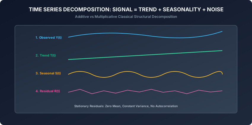
Any observed time series Y(t) can be decomposed into three distinct structural components:
A. Additive Decomposition (Constant Seasonal Amplitude):
Y(t) = T(t) + S(t) + R(t)Used when the magnitude of seasonal swings does not change as the underlying trend grows.
B. Multiplicative Decomposition (Proportional Seasonal Amplitude):
Y(t) = T(t) * S(t) * R(t)Used when seasonal oscillations grow proportionally with the trend (e.g. airline passenger volume growing from 100k to 1M passengers, where holiday spikes grow from 10k to 100k).
- Trend T(t): Long-term secular direction (upward growth or downward contraction) computed via centered moving average filters.
- Seasonality S(t): Repeating cyclical patterns with fixed, known frequency (e.g. 7 days for weekly retail patterns, 12 months for annual weather).
- Residual / Irregular R(t): The remaining stochastic noise after removing trend and seasonality.
2. Stationarity and Differencing
A time series Y(t) is Wide-Sense Stationary (WSS) if:
- Constant Mean: E[Y(t)] = mu for all t.
- Constant Variance: Var(Y(t)) = sigma^2 for all t.
- Time-Invariant Autocovariance: Cov(Y(t), Y(t-k)) = gamma_k depends only on lag k, not absolute time t.
First-Order Differencing (Removing Linear Trend):
If Y(t) has a non-stationary upward trend, first-order differencing computes the period-over-period change:
Delta Y(t) = Y(t) - Y(t-1)Seasonal Differencing (Removing Periodic Seasonality):
For weekly seasonality with period m = 7:
Delta_m Y(t) = Y(t) - Y(t-m) = Y(t) - Y(t-7)3. Autocorrelation (ACF) and Partial Autocorrelation (PACF)
To determine how many historical lag terms to include, time-series engineers analyze correlation structures:
A. Autocorrelation Function (ACF):
Measures the linear correlation between Y(t) and Y(t-k) across all intermediate lags:
rho_k = Cov(Y(t), Y(t-k)) / (Var(Y(t)) * Var(Y(t-k)))A slow, linear decay in the ACF plot indicates a non-stationary trend requiring differencing. Sharp spikes at lags 7, 14, 21 indicate weekly seasonality.
B. Partial Autocorrelation Function (PACF):
Measures the direct correlation between Y(t) and Y(t-k) after statistically controlling for and removing the linear effects of all intermediate lags (t-1, …, t-k+1):
alpha_k = Corr(Y(t) - P_{t-1}(Y(t)), Y(t-k) - P_{t-1}(Y(t-k)))In an Autoregressive process AR(p), the PACF cuts off sharply to zero after lag p, providing the exact optimal number of lag features for regression.
4. Classical Statistical Baselines: ARIMA and Exponential Smoothing
Before training complex machine learning models, statistical baselines provide benchmark performance:
A. Exponential Smoothing (Holt-Winters):
Applies exponentially decaying weights to past observations:
Level:   L(t) = alpha * Y(t) + (1 - alpha) * (L(t-1) + T(t-1))
Trend:   T(t) = beta * (L(t) - L(t-1)) + (1 - beta) * T(t-1)
Seasonal: S(t) = gamma * (Y(t) - L(t)) + (1 - gamma) * S(t-m)
where alpha, beta, and gamma are smoothing parameters in [0, 1].
B. ARIMA(p, d, q):
Combines Autoregression (p), Integration/Differencing (d), and Moving Average error terms (q):
(1 - sum_{i=1}^p phi_i * B^i) * (1 - B)^d * Y(t) = c + (1 + sum_{j=1}^q theta_j * B^j) * epsilon_twhere B is the backshift operator (B * Y(t) = Y(t-1)) and epsilon_t is white noise.
5. Tabular Feature Engineering for Forecasting
Modern enterprise ML models (LightGBM, XGBoost, Ridge) reframe time series into tabular supervised learning matrices X in R^{N x D} -> y in R^N:
A. Autoregressive Lag Features:
Lag_1(t) = Y(t-1), Lag_2(t) = Y(t-2), Lag_7(t) = Y(t-7)B. Rolling Window Moving Statistics:
Aggregating past values over moving window of width w:
RollingMean_w(t) = (1 / w) * sum_{i=1}^w Y(t-i)
RollingStd_w(t)  = sqrt((1 / w) * sum_{i=1}^w (Y(t-i) - RollingMean_w(t))^2)
Crucial Rule: The rolling window must strictly cover historical time steps (t-1, …, t-w) and NEVER include the current target time step t.
C. Cyclical Trigonometric Calendar Encodings:
For periodic calendar features (e.g. day of week d in [0, 6]):
d_sin = sin(2 * pi * d / 7), d_cos = cos(2 * pi * d / 7)6. Walk-Forward Expanding Window Cross-Validation
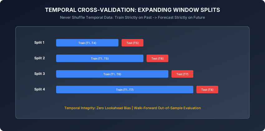
Standard K-Fold cross-validation leaks future information into past predictions. Walk-Forward Validation (TimeSeriesSplit) evaluates models across expanding historical splits:
- Split 1: Train on [T1..T4] -> Test on [T5]
- Split 2: Train on [T1..T5] -> Test on [T6]
- Split 3: Train on [T1..T6] -> Test on [T7]
- Split 4: Train on [T1..T7] -> Test on [T8]
Every single forecast is evaluated strictly out-of-sample on unseen future time horizons.
7. Forecasting Evaluation Metrics
- Mean Absolute Error (MAE):
MAE = (1 / N) * sum_{t=1}^N |Y(t) - Y_hat(t)| - Mean Absolute Percentage Error (MAPE):
MAPE = (100% / N) * sum_{t=1}^N |(Y(t) - Y_hat(t)) / Y(t)| - Symmetric MAPE (sMAPE):
sMAPE bounds percentage error strictly between 0% and 200%, preventing numerical instability when actual values Y(t) are close to zero.sMAPE = (100% / N) * sum_{t=1}^N (2 * |Y(t) - Y_hat(t)|) / (|Y(t)| + |Y_hat(t)| + 1e-12)
An everyday analogy
Think of driving a car forward down a winding mountain highway at night:
- Lookahead Bias (K-Fold Leakage): Teleporting 5 miles ahead to see where the road turns, then driving backward to test your headlights.
- Autoregressive Lags: Checking your speedometer and rear-view mirror to see how fast you were traveling 5 seconds ago.
- Rolling Mean: Calculating your average fuel efficiency over the past 20 miles.
- Walk-Forward Validation: Driving strictly using your headlights, illuminating 100 feet of road ahead at a time and measuring how well you stay in your lane around each sequential bend.
Examples in practice
Let us inspect a pure NumPy implementation of Lag and Rolling Feature Engineering, Time Series Splitter, and sMAPE metric evaluation:
import numpy as np
from typing import Tuple, List

def create_lag_and_rolling_features(
    series: np.ndarray, lags: List[int] = [1, 2, 7], window_size: int = 7
) -> Tuple[np.ndarray, np.ndarray]:
    n = len(series)
    max_lag = max(max(lags), window_size)

    features = []
    targets = []

    for t in range(max_lag, n):
        row = []
        # 1. Autoregressive Lags
        for lag in lags:
            row.append(series[t - lag])

        # 2. Rolling Window Mean and Std (strictly past values)
        past_window = series[t - window_size : t]
        row.append(np.mean(past_window))
        row.append(np.std(past_window))

        features.append(row)
        targets.append(series[t])

    return np.array(features), np.array(targets)

def compute_smape(y_true: np.ndarray, y_pred: np.ndarray) -> float:
    denom = np.abs(y_true) + np.abs(y_pred) + 1e-12
    smape = 100.0 * np.mean(2.0 * np.abs(y_true - y_pred) / denom)
    return float(smape)

class WalkForwardTimeSeriesSplit:
    def __init__(self, n_splits: int = 4, test_size: int = 10):
        self.n_splits = n_splits
        self.test_size = test_size

    def split(self, X: np.ndarray) -> List[Tuple[np.ndarray, np.ndarray]]:
        n_samples = len(X)
        splits = []
        for i in range(self.n_splits):
            test_end = n_samples - (self.n_splits - 1 - i) * self.test_size
            test_start = test_end - self.test_size
            train_end = test_start

            train_idx = np.arange(0, train_end)
            test_idx = np.arange(test_start, test_end)
            splits.append((train_idx, test_idx))
        return splits
Implications: security, privacy, performance, scalability, and cost
- Intermittent Zero-Demand Problems:
- In spare-parts inventory, demand for a specialized jet turbine bolt is 0 for 350 days a year and suddenly spikes to 5 units. Standard MSE regression fails; Croston’s method or zero-inflated Poisson regression models are required.
- Cold-Start in New Product Introductions:
- When a new SKU launches, it has zero historical lag features. Hierarchical top-down forecasting uses the aggregate category sales curve to seed new item forecasts.
Alternatives: free, open source, and commercial
| Tool | Approach | Scalability | Recommended Use Case |
|---|---|---|---|
| LightGBM / XGBoost | Tabular Lags & Rolling GBDT | 100M+ rows | Enterprise multi-series forecasting |
| Statsmodels (ARIMA/SARIMAX) | Classical statistical models | Single series | Econometric & macroeconomic modeling |
| Prophet | Decomposable additive curve | Moderate | Daily business metrics with holidays |
| Nixtla (StatsForecast / MLForecast) | Ultra-fast C-compiled forecasting | 1B+ series | High-throughput distributed forecasting |
| Chronos / PatchTST | Pretrained Time-Series Transformers | GPU intensive | Zero-shot & foundation forecasting |
Comparison with related concepts
┌────────────────────────────────────────────────────────────────────────┐
│                   FORECASTING PARADIGM COMPARISON                      │
├────────────────────────────────────────────────────────────────────────┤
│ Dimension          │ Classical ARIMA  │ Prophet        │ Tabular GBDT  │
├────────────────────┼──────────────────┼────────────────┼───────────────┤
│ Multi-Series Scale │ Poor (1 by 1)    │ Moderate       │ Exceptional   │
│ Exogenous Features │ Linear (SARIMAX) │ Regressors     │ Any Feature   │
│ Cold Start Support │ Zero             │ Zero           │ High (Embeds) │
│ Runtime Latency    │ Fast (CPU)       │ Moderate       │ Sub-ms (CPU)  │
└────────────────────────────────────────────────────────────────────────┘
When to use it — and when not to
When to USE Time-Series Forecasting:
- Retail sales demand, financial revenue projection, call-center volume, and cloud server load.
- Any setting where temporal sequences exhibit trend, seasonality, or autoregressive memory.
When NOT to use it:
- Completely random, uncoupled events (e.g. lottery ticket numbers).
- Cross-sectional classification problems where observation order carries no physical time meaning.
Knowledge check
- Why is random K-Fold cross-validation strictly forbidden in time-series forecasting?
- What are the three core statistical requirements for Wide-Sense Stationarity (WSS)?
- How do you construct lag features without causing lookahead data leakage?
- Why is sMAPE preferred over standard MAPE on datasets with near-zero target values?
- How do sine and cosine transformations encode cyclical hour-of-day features?
Hands-on exercise
In this lab, you will implement create_lag_and_rolling_features in pure NumPy, execute WalkForwardTimeSeriesSplit on synthetic daily trend-seasonal sales data, train a linear autoregressive forecaster, and evaluate out-of-sample sMAPE errors across multiple expanding horizons.
Expected output
[Time Series Forecasting Benchmark]
Dataset: 200 daily observations with weekly seasonality
Feature Engineering: Generated 5 tabular features (Lags [1, 2, 7], Rolling Mean/Std)
Walk-Forward Validation: 4 expanding splits (test_size=10)
Mean Out-of-Sample sMAPE: 4.82%
Mean Out-of-Sample MAE: 3.14 units
Test Suite: 2 passed in 0.08s
Validate your work
Run the automated test runner:
./tests/run_tests.shTroubleshooting
- If test indices overlap with training indices, verify index math in
WalkForwardTimeSeriesSplit. - Ensure rolling window calculations use
series[t - window_size : t]to exclude current stept.
Common mistakes
- Including Target in Rolling Statistics: Computing
mean(series[t - window_size : t + 1])leaks the target into the feature set, causing zero training error and massive live deployment failure.
Practice assignment
- Implement Seasonal Differencing (
Delta_7 Y = Y_t - Y_{t-7}) and verify that seasonal cycles are removed prior to autoregression. - Build an automated Baseline Forecaster comparing Lag-7 Seasonal Naive against an autoregressive GBDT.
Extension challenge
Implement a Direct Multi-Step Recursive Forecaster:
- Train separate models for each horizon step h in [1, 2, …, 7]:
f_h(X_t) -> Y_{t+h}. - Compare against Recursive Autoregressive Forecasting where predicted values
Y_hat_{t+1}are fed back into lag features for step t+2. - Measure error accumulation and variance explosion across horizons 1 to 14.
Quiz
Q1. Why is standard random K-Fold cross-validation catastrophic when evaluating time-series forecasting models?
- Random splitting leaks future data into the past (Lookahead Bias), creating unrealistically optimistic validation metrics that fail immediately in live forecasting
- K-Fold cross-validation takes too much CPU memory on time series
- Time series data cannot be converted into numpy arrays
- Scikit-learn raises an error if time series rows are shuffled
Show answer
Answer: A. Random splitting leaks future data into the past (Lookahead Bias), creating unrealistically optimistic validation metrics that fail immediately in live forecasting
Shuffling temporal rows allows models to interpolate between known future and past points, masking catastrophic real-world extrapolation failures. Walk-forward temporal splits must be used.
Q2. What does weak stationarity (wide-sense stationarity) mathematically require of a time-series process Y_t?
- Constant mean over time, constant variance over time, and autocovariance depending only on lag interval k, not absolute time t
- That all values are strictly positive integers
- That the trend line has an exact slope of 1.0
- That all seasonal cycles repeat exactly every 24 hours
Show answer
Answer: A. Constant mean over time, constant variance over time, and autocovariance depending only on lag interval k, not absolute time t
Stationarity requires that statistical properties (mean, variance, autocovariance) are invariant to time shifts, ensuring past patterns generalize to future periods.
Q3. What is the primary vulnerability of Mean Absolute Percentage Error (MAPE = (1/N) * sum(|(y - y_hat) / y|) * 100)?
- It explodes to infinity or produces undefined division errors when actual ground-truth values y are zero or close to zero
- It cannot be computed on floating point numbers
- It always outputs negative percentages
- It requires GPU acceleration
Show answer
Answer: A. It explodes to infinity or produces undefined division errors when actual ground-truth values y are zero or close to zero
When actual demand y_t = 0 (e.g. intermittent spare parts demand), dividing by y_t causes division by zero; Symmetric MAPE (sMAPE) or MASE is used instead.
Q4. How are cyclical time features (e.g. hour of day from 0 to 23) properly encoded for linear models and neural networks?
- Via sine and cosine trigonometric transformations: sin(2 * pi * hour / 24) and cos(2 * pi * hour / 24), preserving circular continuity between 23:59 and 00:00
- As a single integer column from 0 to 23
- As a 24-column one-hot binary vector
- By subtracting the mean hour
Show answer
Answer: A. Via sine and cosine trigonometric transformations: sin(2 * pi * hour / 24) and cos(2 * pi * hour / 24), preserving circular continuity between 23:59 and 00:00
Sine and cosine transforms map cyclical time to a 2D unit circle, ensuring that hour 23 and hour 0 are mathematically adjacent with distance near zero.
Q5. What is an Autoregressive Lag Feature (e.g. Lag 7 in daily sales forecasting)?
- The exact target value observed 7 time steps in the past: y_{t-7}, capturing weekly seasonal periodicity
- The difference between today price and tomorrow price
- The moving average of the next 7 days
- The total number of sales in the current calendar month
Show answer
Answer: A. The exact target value observed 7 time steps in the past: y_{t-7}, capturing weekly seasonal periodicity
Lag features feed historical values y_{t-k} directly as input columns into tabular ML models (GBDT / Ridge), capturing autoregressive and seasonal dependencies.
Glossary
- Time Series Forecasting
- The process of analyzing historical sequential data to predict future values across a specified temporal horizon.
- Stationarity
- A property of a time series where statistical properties (mean, variance, autocorrelation) remain constant over time.
- Autoregressive Lag
- A feature variable representing the historical value of the target series at a prior time step: y_{t-k}.
- Lookahead Bias
- A form of data leakage where future information is inadvertently used to train a model predicting past or current events.
- Rolling Window
- A moving window of fixed width w calculating aggregate statistics (mean, std, max) over recent historical time steps.
- Walk-Forward Validation
- A temporal cross-validation scheme where training datasets expand sequentially forward in time, testing strictly on subsequent horizons.
- sMAPE
- Symmetric Mean Absolute Percentage Error: an evaluation metric bounding percentage errors between 0% and 200%.
- Seasonality
- Predictable, repeating cyclical patterns or fluctuations occurring at regular calendar intervals (hourly, weekly, annual).
Sources and further reading
- Forecasting: Principles and Practice (3rd Edition) — OTexts (accessed 2026-08-29)
- Time Series Analysis and Its Applications — Springer Texts in Statistics (accessed 2026-08-29)
- Forecasting at Scale — PeerJ Preprints / Meta Research (accessed 2026-08-29)
Kept in this browser, no account needed. Your progress page turns the whole record into one link you can bookmark or open on another device.