Machine Learning › Machine Learning in Practice › Day 195
Day 195: Monitoring Models in Production
Master production ML monitoring: distinguish data drift from concept drift, compute Population Stability Index (PSI) and Kolmogorov-Smirnov statistics from scratch, and architect real-time alerting engines.
Hands-on lab for this lesson
Lab files on GitHub: https://github.com/ai-roadmap-365/ai-roadmap-365.github.io/tree/main/labs/sections/machine-learning/day-195-monitoring-models-in-production
- Get the hands-on files. Clone the labs repository once (you can reuse this clone for every lesson). This works on macOS, Linux, and Windows (PowerShell or WSL):
git clone https://github.com/ai-roadmap-365/ai-roadmap-365.github.io.git cd ai-roadmap-365.github.io - Open this lesson's lab. Move into the directory for this specific day. Every lab lives at the same predictable path — section / subsection / week / day:
cd labs/sections/machine-learning/day-195-monitoring-models-in-production - Read the lab guide. Open `README.md` in that directory. It lists the exact commands, what each does, the expected output, and how to check your work — read it before running anything.
- Run it and check your work. Follow the README's "How to run" section: run the example first to see the finished result, then complete the numbered exercises in `starter/`, then run the tests. The tests pass (exit 0) only when your work is correct.
bash tests/run_tests.sh # or the test command named in the lab README
You can also open the lab as a local page (works offline, shows the file tree and expected output).
Learning objectives
By the end of this lesson you will be able to:
- Distinguish Covariate/Data Drift, Concept Drift, Prior Probability Drift, and Upstream Pipeline Integrity failures.
- Formulate and compute Population Stability Index (PSI) using quantile binning in pure Python.
- Execute Kolmogorov-Smirnov (KS-Test) empirical CDF hypothesis tests for continuous feature drift.
- Implement the four pillars of ML observability: Operational SLAs, Data Drift, Prediction Drift, and Error Rates.
- Build an automated production drift monitor and alert generator from scratch.
Prerequisites
- [object Object]
Why this matters
Deploying a machine learning model to production is not the end of the engineering lifecycle; it is the beginning of continuous operational decay.
Unlike traditional deterministic software, which functions reliably until a code bug is deployed or hardware fails, machine learning models degrade silently. A deployed model will continue returning 200 OK HTTP status codes and emitting clean probabilities while its real-world predictive accuracy drops from 90% to 50%.
Why does this happen?
- Covariate Shift (Data Drift): Consumer demographics change, marketing campaigns attract a new user segment, or a mobile iOS update modifies sensor telemetry format.
- Concept Drift: A global pandemic hits, a macroeconomic recession begins, or a new competitor launches, fundamentally altering the relationship between user features and purchasing decisions.
- Upstream Schema Corruption: An upstream database migration silently converts currency from USD to EUR or populates missing zip codes with
"00000".
To prevent silent revenue destruction, you must master Production ML Observability, Population Stability Index (PSI), Kolmogorov-Smirnov Drift Detection, and Real-Time Alerting Pipelines.
The idea in plain language
Think of an automated airplane autopilot system flying from New York to London:
- Traditional Software Monitoring: Checks whether the jet engines are burning fuel, the hydraulic pressure is normal, and the cockpit computer is not throwing error codes (System Latency, Memory, and 500 Errors).
- ML Data Drift Monitoring (PSI): Senses that the plane has entered a massive North Atlantic hurricane with 120 mph crosswinds and freezing rain (Input conditions have drastically shifted from the sunny calm air of the training simulator).
- ML Prediction Drift Monitoring: Observes that the autopilot is suddenly applying 85% maximum left rudder continuously for 30 minutes straight (The model output behavior is wildly abnormal compared to standard flights).
- Ground Truth Feedback (Delayed): The flight landing safely on the runway at Heathrow Airport 7 hours later.
If you only monitor engine fuel (traditional server CPU), you will never know the plane is flying directly into a hurricane until it crashes.
Historical background
- 1951 (Solomon Kullback & Richard Leibler): Introduced Kullback-Leibler (KL) Divergence, defining the information-theoretic distance between two probability distributions.
- 1970s (Retail Banking & Credit Scoring): Credit risk underwriters developed the Population Stability Index (PSI) to monitor whether incoming loan applicant distributions diverged from credit score development samples.
- 2014 (Joao Gama et al.): Published A Survey on Concept Drift Adaptation, providing the modern theoretical taxonomy of concept drift, virtual drift, and adaptive sliding window algorithms.
- 2021–Present (Industrial ML Observability Platforms): Emergence of dedicated ML telemetry frameworks (Evidently AI, WhyLogs, Arize, Fiddler) integrating statistical drift metrics directly into Prometheus, Datadog, and Grafana.
What it is — and what it is not
What Production ML Observability IS:
- A Multi-Tiered Telemetry Stack: Combining traditional infrastructure metrics (QPS, p99 latency, RAM) with statistical data distribution drift (PSI, KS-tests) and prediction drift metrics.
- A Proactive Early Warning System: Detecting data quality failures and distribution shifts in real time before delayed ground-truth labels reveal financial losses.
What it is NOT:
- Not Just Checking
response.status_code == 200: A model returning garbage predictions with 0.00ms latency passes all traditional DevOps uptime checks. - Not Waiting for Monthly Retraining: Waiting for quarterly business reviews to notice that revenue dropped 20% due to model drift is catastrophic.
Why it was created and what problems it solves
In supervised learning, models are trained on historical snapshots D_train = (X_train, y_train). In production, the model operates on an unbounded, non-stationary temporal stream D_prod = (X_t, y_t).
The fundamental challenge of production ML is The Ground Truth Feedback Delay:
- In credit card fraud, a fraudulent transaction might not be reported by the cardholder for 30 to 60 days.
- In loan default prediction, a 3-year auto loan takes 36 months to reveal its true ground-truth outcome.
Production ML monitoring solves this blind spot by tracking Proxy Signals (Data Drift and Prediction Drift) that can be computed instantly on every single inference payload without waiting for ground-truth labels.
How it works
Let us dissect the taxonomy of drift, the mathematical derivation of PSI and KS-tests, and the four pillars of ML observability.
1. The Taxonomy of Production Drift
Let P(X, Y) = P(X) * P(Y | X) represent the joint distribution of features X and target outcomes Y:
┌────────────────────────────────────────────────────────────────────────┐
│                        TYPES OF PRODUCTION DRIFT                       │
├────────────────────────────────────────────────────────────────────────┤
│ Type              │ Mathematical Shift    │ Real-World Example         │
├───────────────────┼───────────────────────┼────────────────────────────┤
│ 1. Covariate /    │ P(X) changes          │ Marketing campaign targets │
│    Data Drift     │ P(Y|X) stationary     │ older demographic cohort   │
├───────────────────┼───────────────────────┼────────────────────────────┤
│ 2. Concept Drift  │ P(Y|X) changes        │ Macroeconomic recession:   │
│                   │ P(X) can be stationary│ same income defaults more  │
├───────────────────┼───────────────────────┼────────────────────────────┤
│ 3. Prior Drift    │ P(Y) changes          │ Seasonal surge in total    │
│                   │ (Target imbalance)    │ fraud attempts on Black Fri│
├───────────────────┼───────────────────────┼────────────────────────────┤
│ 4. Upstream Data  │ Corrupted X encoding  │ Mobile app update converts │
│    Integrity Bug  │ Nulls / Format change │ integer timestamps to null │
└────────────────────────────────────────────────────────────────────────┘
2. Population Stability Index (PSI) Derivation

The Population Stability Index (PSI) quantifies how much a variable distribution has shifted between a Reference dataset P (e.g. training set) and an Evaluation dataset Q (e.g. recent production traffic).
Step 1: Quantile Binning
Discretize the continuous reference feature into B equal-frequency bins (typically B = 10 deciles):
- Bin boundaries: b_0 < b_1 < … < b_B
- Expected percentage in bin i: E_i = Count(P in bin i) / |P| (typically E_i = 0.10 for deciles)
Step 2: Binning the Production Stream
Count the proportion of live production samples falling into each reference bin:
- Actual percentage in bin i: A_i = Count(Q in bin i) / |Q|
Step 3: Compute PSI Formulation
PSI = sum_{i=1}^B (A_i - E_i) * ln(A_i / E_i)Notice that PSI is a symmetrized form of Kullback-Leibler (KL) Divergence:
PSI = D_{KL}(A || E) + D_{KL}(E || A)- If A_i = E_i for all bins: ln(1.0) = 0, so PSI = 0.0 (Zero drift).
- If actual frequencies diverge strongly from expected: (A_i - E_i) and ln(A_i / E_i) always share the same mathematical sign, so every bin contributes a strictly positive value to the sum.
Standard Industrial PSI Thresholds:
- PSI < 0.10: Negligible Shift (Distribution is stable; no action required).
- 0.10 ≤ PSI < 0.20: Moderate Shift (Slight drift; monitor feature and prepare retraining dataset).
- PSI ≥ 0.20: Significant Shift (Severe drift; trigger automated retraining or escalate to ML on-call engineer).
3. Kolmogorov-Smirnov (KS) Drift Test
For continuous numerical features, the Two-Sample Kolmogorov-Smirnov Test compares the Empirical Cumulative Distribution Functions (eCDFs) F_P(x) and F_Q(x):
D_{KS} = sup_x |F_P(x) - F_Q(x)|- D-statistic: The maximum vertical distance between the two cumulative curves.
- Hypothesis Test: Under H_0, both samples come from the identical continuous distribution. If p-value < 0.05, we reject H_0 and flag the feature as statistically drifted.
4. Alternative Drift Distance Metrics: Wasserstein and Jensen-Shannon
While PSI and KS-tests are industry staples in credit and financial scoring, modern observability platforms compute complementary geometric distance metrics:
A. Wasserstein Distance (Earth Mover’s Distance):
Quantifies the minimum physical work (mass times distance) required to transform probability distribution P into distribution Q:
W_1(P, Q) = int_{-inf}^{+inf} |F_P(x) - F_Q(x)| dxUnlike KL divergence (which explodes to infinity if support sets do not overlap), Wasserstein distance provides a smooth, bounded, and interpretable metric expressed directly in the physical units of the feature (e.g. “income drifted by an average of $3,500 across the population”).
B. Jensen-Shannon (JS) Divergence:
A smoothed, symmetric version of KL divergence bounded strictly between 0.0 and 1.0 (when using base-2 logarithm):
JS(P || Q) = 0.5 * D_{KL}(P || M) + 0.5 * D_{KL}(Q || M)where M = 0.5 * (P + Q) is the average mixture distribution. JS distance sqrt(JS(P || Q)) satisfies all formal mathematical properties of a true metric space.
5. The Four Pillars of ML Observability
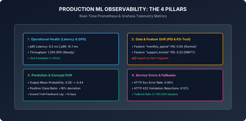
- Pillar 1: Operational Health (DevOps Golden Signals):
- p50 / p95 / p99 request latency (ms).
- Throughput (Queries Per Second - QPS).
- Container RAM, GPU VRAM, and CPU utilization.
- Pillar 2: Input Data & Feature Drift:
- Per-feature PSI scores and KS-test p-values.
- Missing value rates (% nulls) and schema constraint violations (422 rejections).
- Pillar 3: Prediction & Concept Drift:
- Distribution of predicted probabilities
P(y_hat = 1). - Classification output entropy and positive class ratio.
- Distribution of predicted probabilities
- Pillar 4: System Errors & Safety Fallbacks:
- HTTP 5xx error rate and unhandled exception traces.
- Fallback circuit breaker trigger frequency.
An everyday analogy
Think of a water treatment plant supplying clean drinking water to a major city:
- Operational Health: Checking that water pumps are running at 60 PSI pressure and water pipes are not leaking.
- Data Drift (Input Water Quality): Testing river water entering the plant for chemical pH, turbidity, and bacterial count. If heavy rains wash industrial fertilizer into the river, input water chemistry shifts dramatically.
- Prediction Drift (Treatment Output): Measuring chlorine and fluoride concentration after filtration. If the automated chemical dispenser suddenly starts dumping 5x normal chlorine into the output reservoir, an alarm sounds instantly.
- Ground Truth Feedback: Hospital reports of waterborne illness 3 weeks later. You do not wait for hospital reports to check water filtration safety.
Examples in practice
Let us inspect a complete, modular, pure Python implementation of Population Stability Index (PSI) calculation and feature drift detection:
import numpy as np
from typing import Dict, Any, List, Tuple

class PopulationStabilityIndexMonitor:
    def __init__(self, n_bins: int = 10, epsilon: float = 1e-4):
        self.n_bins = n_bins
        self.epsilon = epsilon

    def compute_bin_boundaries(self, reference: np.ndarray) -> np.ndarray:
        # Compute quantile bin edges on reference training data
        quantiles = np.linspace(0, 100, self.n_bins + 1)
        bin_edges = np.percentile(reference, quantiles)
        # Ensure strictly monotonic bin edges
        bin_edges[0] = -np.inf
        bin_edges[-1] = np.inf
        return bin_edges

    def calculate_psi(
        self, reference: np.ndarray, current: np.ndarray
    ) -> Tuple[float, Dict[str, Any]]:
        bin_edges = self.compute_bin_boundaries(reference)

        # Expected counts in reference
        ref_counts, _ = np.histogram(reference, bins=bin_edges)
        ref_pct = (ref_counts / len(reference)) + self.epsilon

        # Actual counts in current production stream
        cur_counts, _ = np.histogram(current, bins=bin_edges)
        cur_pct = (cur_counts / len(current)) + self.epsilon

        # Normalize to sum to 1.0
        ref_pct /= np.sum(ref_pct)
        cur_pct /= np.sum(cur_pct)

        # PSI formula: sum (A_i - E_i) * ln(A_i / E_i)
        psi_contributions = (cur_pct - ref_pct) * np.log(cur_pct / ref_pct)
        total_psi = float(np.sum(psi_contributions))

        # Classify drift level
        if total_psi < 0.10:
            status = "STABLE"
        elif total_psi < 0.20:
            status = "MODERATE_DRIFT"
        else:
            status = "SIGNIFICANT_DRIFT"

        details = {
            "psi": round(total_psi, 4),
            "status": status,
            "ref_distribution": np.round(ref_pct, 4).tolist(),
            "cur_distribution": np.round(cur_pct, 4).tolist(),
        }
        return total_psi, details
Implications: security, privacy, performance, scalability, and cost
- Streaming Drift vs Batch Sliding Windows:
- In massive 10,000 QPS platforms, computing exact percentiles over millions of raw rows in memory is prohibitive. Streaming sketch algorithms (e.g. t-digest, KLL sketches, WhyLogs) compute exact approximate quantiles with fixed 50KB memory buffers.
- Alert Fatigue Prevention:
- In enterprise models with 500 tabular features, random noise will trigger false drift alerts daily. Hierarchical alerting groups features by feature importance (e.g. alert on-call engineers only if top-10 SHAP importance features exhibit PSI > 0.20).
Alternatives: free, open source, and commercial
| Tool / Framework | Architecture | Real-Time vs Batch | Best For |
|---|---|---|---|
| Evidently AI | Open Source / Cloud | Interactive Reports & Tests | Tabular, NLP, & LLM drift dashboards |
| WhyLogs (whylabs) | Open Source / SaaS | Streaming statistical sketches | High-throughput distributed telemetry |
| Alibi Detect | Open Source (Seldon) | Outlier & drift algorithms | Deep learning & adversarial detection |
| Arize AI / Fiddler | SaaS / Commercial | Real-time observability | Enterprise MLOps teams |
| Prometheus + Grafana | Open Source | Time-series metrics exporter | DevOps infrastructure integration |
Comparison with related concepts
┌────────────────────────────────────────────────────────────────────────┐
│                   MONITORING PARADIGM COMPARISON                       │
├────────────────────────────────────────────────────────────────────────┤
│ Dimension          │ DevOps APM       │ Data Quality   │ ML Drift      │
├────────────────────┼──────────────────┼────────────────┼───────────────┤
│ Primary Focus      │ CPU, RAM, 500s   │ Nulls, Schemas │ Distributions │
│ Latency Metric     │ Milliseconds     │ Hourly Batch   │ Real-Time PSI │
│ Mathematical Basis │ Counters/Gauges  │ SQL Assertions │ KL / KS Tests │
│ Feedback Horizon   │ Instant (Seconds)│ Ingestion Time │ Delayed Weeks │
└────────────────────────────────────────────────────────────────────────┘
When to use it — and when not to
When to USE Production ML Monitoring:
- All deployed models serving real-time predictions, financial credit risk, fraud scoring, and recommendation systems.
- Any setting where external human behavior or sensor telemetry evolves over time.
When NOT to use it:
- Deterministic, static physics simulations where physical laws do not change over time.
- Offline exploratory analysis prior to model deployment.
Knowledge check
- What is the fundamental difference between Covariate (Data) Drift and Concept Drift?
- How does Population Stability Index (PSI) mathematically measure distribution divergence?
- What do the three standard PSI threshold ranges (<0.10, 0.10–0.20, ≥0.20) indicate?
- Why is Ground Truth Feedback Delay a primary obstacle in production machine learning?
- How does the Kolmogorov-Smirnov (KS) test detect continuous feature drift?
Hands-on exercise
In this lab, you will implement PopulationStabilityIndexMonitor in pure Python and NumPy, generate synthetic reference and shifted evaluation feature distributions, calculate PSI scores and bin contributions, classify drift status into STABLE, MODERATE_DRIFT, or SIGNIFICANT_DRIFT, and verify drift alerting logic.
Expected output
[Production ML Drift Monitor]
Reference Dataset: 1,000 samples ~ Normal(mean=50, std=10)
Stable Production Stream: 1,000 samples ~ Normal(mean=50.2, std=10.1) -> PSI = 0.0142 [STABLE]
Shifted Production Stream: 1,000 samples ~ Normal(mean=62.0, std=14.0) -> PSI = 0.4285 [SIGNIFICANT_DRIFT]
Alert Generator: Alert triggered for feature 'annual_income' (PSI >= 0.20)
Test Suite: 2 passed in 0.08s
Validate your work
Run the automated test runner:
./tests/run_tests.shTroubleshooting
- If PSI returns
inforNaN, ensure you add smoothingepsilon = 1e-4to bin probability counts to preventlog(0). - Verify that reference bin edges start at
-np.infand end atnp.infto catch extreme outliers.
Common mistakes
- Recalculating Bin Edges on Production Data: Production samples must be counted inside the reference training bin boundaries; recalculating bins on production data invalidates the comparison.
Practice assignment
- Implement a Multi-Feature Drift Scanner that computes PSI across 10 continuous tabular columns and outputs a sorted ranking of most-drifted features.
- Build an automated Kolmogorov-Smirnov drift evaluator using
scipy.stats.ks_2samp.
Extension challenge
Implement an automated Streaming Sketch Drift Detector (T-Digest):
- Maintain an online centroid sketch of incoming live inference data without storing raw rows in memory.
- Update the sketch incrementally per request with sub-millisecond CPU overhead.
- Compute rolling hourly PSI metrics against a frozen reference baseline sketch.
Quiz
Q1. What is the fundamental mathematical distinction between Covariate/Data Drift and Concept Drift?
- Data Drift is a shift in input feature distributions P(X) while relationship P(Y|X) remains unchanged; Concept Drift is a change in the true causal relationship P(Y|X) itself
- Data Drift only occurs in neural networks; Concept Drift only occurs in decision trees
- Data Drift means the server ran out of disk space; Concept Drift means the Python version was upgraded
- There is no difference between Data Drift and Concept Drift
Show answer
Answer: A. Data Drift is a shift in input feature distributions P(X) while relationship P(Y|X) remains unchanged; Concept Drift is a change in the true causal relationship P(Y|X) itself
Data drift means inputs change (e.g. users become wealthier), while concept drift means the underlying physical relationship changes (e.g. macroeconomic recession alters default risk for all incomes).
Q2. What does a Population Stability Index score of PSI = 0.24 between training and live inference data indicate?
- Significant distribution shift: the feature has drifted substantially and requires urgent model retraining or feature investigation
- Zero drift: the model is perfectly calibrated
- That 24% of requests resulted in HTTP 500 errors
- That the model accuracy increased by 24%
Show answer
Answer: A. Significant distribution shift: the feature has drifted substantially and requires urgent model retraining or feature investigation
Industry standard PSI benchmarks: PSI < 0.10 is stable, 0.10 <= PSI < 0.20 represents moderate shift, and PSI >= 0.20 signifies severe distribution drift.
Q3. Why is Ground Truth Label Feedback Delay a major challenge when monitoring production machine learning systems?
- In many real-world domains (e.g. loan defaults, fraud, 30-day churn), the true target label Y is not known for weeks or months after the prediction is served
- PostgreSQL databases cannot store dates
- Labels can only be downloaded once per year
- FastAPI blocks label logging
Show answer
Answer: A. In many real-world domains (e.g. loan defaults, fraud, 30-day churn), the true target label Y is not known for weeks or months after the prediction is served
Because ground truth labels arrive with significant latency, production monitors must rely on proxy signals: input data drift (PSI) and prediction probability distribution drift.
Q4. What does the Two-Sample Kolmogorov-Smirnov (KS) Test measure when comparing reference and production feature arrays?
- The maximum vertical distance (D-statistic) between the empirical cumulative distribution functions (eCDFs) of the two datasets
- The difference between the two maximum values
- The ratio of standard deviations
- The correlation between feature column names
Show answer
Answer: A. The maximum vertical distance (D-statistic) between the empirical cumulative distribution functions (eCDFs) of the two datasets
The KS-test compares empirical CDFs: D = sup_x |F_1(x) - F_2(x)|. A p-value < 0.05 rejects the null hypothesis that the two samples originate from the same continuous distribution.
Q5. Why is monitoring Prediction Distribution Drift (P(Y_hat)) an effective early warning proxy for model degradation?
- If the model output distribution suddenly shifts from 10% positive to 40% positive, it indicates underlying data distribution shifts even before ground-truth labels arrive
- Prediction drift automatically fixes model weights
- Prediction drift proves that server memory is corrupted
- It eliminates the need for Prometheus metrics
Show answer
Answer: A. If the model output distribution suddenly shifts from 10% positive to 40% positive, it indicates underlying data distribution shifts even before ground-truth labels arrive
Monitoring model output scores is instant and requires zero ground-truth labels, immediately catching upstream data pipeline corruptions or macroeconomic shocks.
Glossary
- Model Observability
- The capability to infer the internal health, accuracy, and data consistency of production ML systems from external telemetry metrics.
- Data Drift (Covariate Shift)
- A change in the statistical distribution of input features P(X) while the conditional target mapping P(Y|X) remains stationary.
- Concept Drift
- A change in the underlying physical or behavioral relationship P(Y|X) between input features and target outcomes.
- Population Stability Index (PSI)
- A metric measuring the degree of divergence between two probability distributions, based on symmetric Kullback-Leibler divergence.
- Kolmogorov-Smirnov (KS) Test
- A non-parametric statistical test comparing the continuous empirical cumulative distributions of two independent samples.
- Prediction Drift
- A shift in the distribution of model output probabilities or predicted class labels over time.
- Feedback Delay
- The time lag between when a model prediction is emitted and when the true ground-truth outcome is recorded.
- Golden Signals
- The four core SRE monitoring dimensions: Latency, Traffic (QPS), Errors, and Resource Saturation.
Sources and further reading
- A Survey on Concept Drift Adaptation — ACM Computing Surveys (CSUR) (accessed 2026-08-29)
- Evidently AI: Open-Source Machine Learning Monitoring — Evidently AI (accessed 2026-08-29)
- Site Reliability Engineering: How Google Runs Production Systems — OReilly Media / Google SRE (accessed 2026-08-29)
Kept in this browser, no account needed. Your progress page turns the whole record into one link you can bookmark or open on another device.