Deep Learning › Neural Network Foundations › Day 197
Day 197: The Perceptron
Master the fundamental building block of Deep Learning: formulate Frank Rosenblatt Artificial Perceptron, prove the Perceptron Learning Rule, analyze linear separability, and overcome the historic XOR barrier.
Hands-on lab for this lesson
Lab files on GitHub: https://github.com/ai-roadmap-365/ai-roadmap-365.github.io/tree/main/labs/sections/deep-learning/day-197-the-perceptron
- Get the hands-on files. Clone the labs repository once (you can reuse this clone for every lesson). This works on macOS, Linux, and Windows (PowerShell or WSL):
git clone https://github.com/ai-roadmap-365/ai-roadmap-365.github.io.git cd ai-roadmap-365.github.io - Open this lesson's lab. Move into the directory for this specific day. Every lab lives at the same predictable path — section / subsection / week / day:
cd labs/sections/deep-learning/day-197-the-perceptron - Read the lab guide. Open `README.md` in that directory. It lists the exact commands, what each does, the expected output, and how to check your work — read it before running anything.
- Run it and check your work. Follow the README's "How to run" section: run the example first to see the finished result, then complete the numbered exercises in `starter/`, then run the tests. The tests pass (exit 0) only when your work is correct.
bash tests/run_tests.sh # or the test command named in the lab README
You can also open the lab as a local page (works offline, shows the file tree and expected output).
Learning objectives
By the end of this lesson you will be able to:
- Derive the mathematical formulation of the McCulloch-Pitts biological neuron and Rosenblatt Artificial Perceptron.
- Implement the Perceptron Learning Rule (weight and bias update equation) from scratch in pure NumPy.
- Prove the Perceptron Convergence Theorem for linearly separable binary classification datasets.
- Analyze the geometric limitation of single-layer hyperplanes and explain Minsky and Papert historic XOR critique.
- Solve linearly non-separable XOR parity by hand-engineering a two-layer Multi-Layer Perceptron (MLP).
Prerequisites
- [object Object]
Why this matters
Welcome to Course 05: Deep Learning!
In Course 04, you mastered classical machine learning algorithms. You built decision trees, evaluated gradient boosted ensembles, tuned hyperplanes with support vector machines, and segmented data using unsupervised manifolds. In all of those algorithms, feature representation was handcrafted by human engineers: you computed logarithms, designed polynomial combinations, and extracted autoregressive lags.
Deep Learning revolutionizes computational intelligence through Representation Learning: instead of manually hand-engineering feature representations, multi-layered artificial neural networks automatically discover hierarchical feature abstractions directly from raw data.
At the heart of every modern deep neural network — from simple multi-layer perceptrons to convolutional vision networks and 100-billion parameter Large Language Model Transformers — lies a single, foundational mathematical atom: The Artificial Perceptron.
Invented by psychologist Frank Rosenblatt in 1958 at Cornell Aeronautical Laboratory, the Perceptron was the very first algorithmic model of a learning biological neuron. Understanding its mathematical mechanics, its convergence guarantees, and its famous geometric limitations (the XOR barrier) is the essential starting point for mastering Deep Learning.
The idea in plain language
Imagine a smart thermostat deciding whether to turn on an air conditioning unit:
- The thermostat receives several sensory inputs:
- x1 (Room Temperature): 78 degrees F (Hot).
- x2 (Humidity): 85% (High).
- x3 (Electricity Price): $0.45 / kWh (Expensive peak rate).
- The thermostat has internal importance dials (Weights w1, w2, w3):
- It assigns high positive weight to temperature (
w1 = +2.0). - It assigns positive weight to humidity (
w2 = +1.0). - It assigns negative weight to electricity cost (
w3 = -3.0).
- It assigns high positive weight to temperature (
- It has an internal baseline comfort threshold (Bias b = -5.0).
- The Decision Math: The thermostat computes a weighted score:
Score = (78 * 2.0) + (85 * 1.0) + (0.45 * -3.0) - 5.0 = 239.65 - If
Score >= 0, the unit fires on (y_hat = 1). IfScore < 0, it stays off (y_hat = 0). - Learning from Mistakes: If the homeowner complains that they are freezing cold, the thermostat adjusts its weights and threshold slightly to prevent future mistakes.
Historical background
- 1943 (Warren McCulloch & Walter Pitts): Published A Logical Calculus of the Ideas Immanent in Nervous Activity, proposing the first mathematical threshold model of a biological neuron.
- 1958 (Frank Rosenblatt): Published The Perceptron: A Probabilistic Model for Information Storage and Organization in the Brain, introducing the Perceptron and the automated Perceptron Learning Rule implemented on the custom Mark I Perceptron hardware computer at Cornell.
- 1962 (Albert Novikoff): Proved the Perceptron Convergence Theorem, establishing that the learning rule is guaranteed to find a separating hyperplane in finite iterations on linearly separable data.
- 1969 (Marvin Minsky & Seymour Papert): Published their influential book Perceptrons, mathematically proving that single-layer perceptrons cannot solve non-linear boolean logic (specifically the XOR parity function). This triggered the first catastrophic AI Winter, freezing neural network funding for over 15 years.
- 1986 (Rumelhart, Hinton, & Williams): Revitalized neural networks by demonstrating that multi-layer networks with continuous activations and Backpropagation seamlessly solve the XOR problem and complex non-linear manifolds.
What it is — and what it is not
What the Perceptron IS:
- A Linear Binary Classifier: A mathematical unit that partitions N-dimensional feature space using an (N-1)-dimensional flat hyperplane.
- An Online Supervised Learning Algorithm: Adjusting its parameters sample-by-sample whenever a misclassification error occurs.
What it is NOT:
- Not a Multi-Layer Deep Neural Network: A single perceptron has zero hidden layers and zero non-linear representational capacity.
- Not Logistic Regression: The classic Rosenblatt perceptron uses a discontinuous step threshold (
y in {0, 1}) rather than a continuous, differentiable logistic sigmoid probability curve.
Why it was created and what problems it solves
Prior to 1958, computational systems were hard-coded: programmers wrote explicit, deterministic logic rules by hand. If an engineer wanted a computer to recognize a handwritten letter “A”, they had to specify exact coordinate positions for every line segment.
Rosenblatt created the Perceptron to answer a profound scientific question: Can a physical machine learn to classify visual sensory patterns automatically through trial and error?
The Perceptron solved this by introducing weight adaptation driven by empirical error feedback.
How it works
Let us dissect the mathematical architecture of the Artificial Perceptron, the Perceptron Learning Rule, the Convergence Theorem, and the XOR linear separability barrier.
1. The Perceptron Architecture
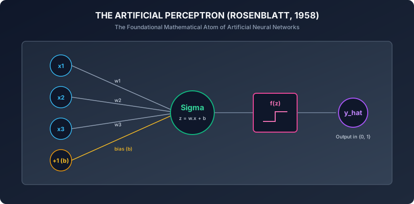
Given an input feature vector x = [x_1, x_2, ..., x_D]^T in R^D:
Step 1: Linear Combination (Pre-Activation)
Compute the dot product of input vector x with weight vector w = [w_1, w_2, ..., w_D]^T plus scalar bias b:
z = sum_{j=1}^D w_j * x_j + b = w^T x + bStep 2: Heaviside Step Activation
Apply the discontinuous step threshold function:
y_hat = f(z) = 1  if z >= 0
             = 0  if z < 0
The geometric decision boundary separating class 0 and class 1 is the linear hyperplane defined by:
w^T x + b = 02. The Perceptron Learning Algorithm
The Perceptron updates its weights and bias iteratively in response to misclassified training samples:
Algorithm:
- Initialize weights
w = [0, 0, ..., 0]^Tand biasb = 0(or small random values). - Choose a learning rate
eta in (0, 1](typicallyeta = 0.1or1.0). - For each training epoch, iterate through training pairs
(x^{(i)}, y^{(i)}):- Compute predicted output:
y_hat^{(i)} = f(w^T x^{(i)} + b). - Compute classification error:
error^{(i)} = y^{(i)} - y_hat^{(i)}. - Update weights and bias:
w_j <- w_j + eta * (y^{(i)} - y_hat^{(i)}) * x_j^{(i)}
b   <- b   + eta * (y^{(i)} - y_hat^{(i)})
- Compute predicted output:
- Repeat until all training samples are classified correctly (
error = 0for all i) or maximum epochs are reached.
The Intuition Behind the Update:
- Case 1: Correct Classification (
y = y_hat): Error is 0. Weights and bias remain unchanged. - Case 2: False Negative (
y = 1, y_hat = 0): Error is+1. The update addseta * xtow, rotating the weight vector towardxand increasingw^T x + bfor the next pass. - Case 3: False Positive (
y = 0, y_hat = 1): Error is-1. The update subtractseta * xfromw, rotating the weight vector away fromxand decreasingw^T x + b.
3. The Perceptron Convergence Theorem (Novikoff, 1962)
If a training dataset D = {(x^{(1)}, y^{(1)}), ..., (x^{(N)}, y^{(N)})} is linearly separable, there exists an optimal unit weight vector w* (with ||w*|| = 1) and a positive margin gamma > 0 such that for all samples:
(2 * y^{(i)} - 1) * (w*^T x^{(i)} + b*) >= gammaLet R = max_i ||x^{(i)}|| be the maximum Euclidean radius of the training inputs.
Novikoff’s Theorem proves that the maximum number of weight updates k before total convergence is strictly bounded by:
k <= (R / gamma)^2Implication: If the data is linearly separable, the Perceptron will 100% guaranteed converge to zero errors in finite steps. If the data is NOT linearly separable, the algorithm will oscillate indefinitely without ever converging.
4. Linear Separability and the XOR Barrier
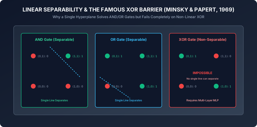
Let us examine why a single-layer perceptron can solve the boolean AND and OR functions, but fails catastrophically on XOR (Exclusive OR):
A. The AND Gate Truth Table:
(0, 0) -> 0(1, 0) -> 0(0, 1) -> 0(1, 1) -> 1Linear Solution:w_1 = 1.0, w_2 = 1.0, b = -1.5. Hyperplanex_1 + x_2 - 1.5 = 0cleanly separates(1, 1)from the rest.
B. The OR Gate Truth Table:
(0, 0) -> 0(1, 0) -> 1(0, 1) -> 1(1, 1) -> 1Linear Solution:w_1 = 1.0, w_2 = 1.0, b = -0.5. Hyperplanex_1 + x_2 - 0.5 = 0cleanly separates(0, 0)from the rest.
C. The XOR Gate Truth Table:
(0, 0) -> 0(1, 0) -> 1(0, 1) -> 1(1, 1) -> 0
In 2D geometric space, the positive points (1, 0) and (0, 1) lie on the opposite diagonal from the negative points (0, 0) and (1, 1). It is mathematically impossible for any single straight line to divide the positive points from the negative points.
To solve XOR, we must compose multiple perceptrons into a Multi-Layer Perceptron (MLP):
- Hidden Neuron 1 computes
NAND(x_1, x_2). - Hidden Neuron 2 computes
OR(x_1, x_2). - Output Neuron computes
AND(Hidden 1, Hidden 2).
XOR(x_1, x_2) = AND(NAND(x_1, x_2), OR(x_1, x_2))The hidden layer maps the 2D non-separable input space into a new feature space where a linear hyperplane can separate the classes.
An everyday analogy
Think of cutting a piece of fruit on a cutting board with a single straight chef’s knife blade:
- Linearly Separable (AND/OR): You have red apples on the left and green limes on the right. You make a single straight chop with your knife, cleanly separating all apples from all limes.
- The XOR Problem: You have 4 fruit pieces arranged in a checkerboard square: top-left is green lime, top-right is red apple, bottom-left is red apple, bottom-right is green lime.
- No matter what single straight angle you slice with your knife, you cannot separate all red apples from all green limes in one cut.
- To separate them, you need two knife cuts (a multi-layer neural network with multiple decision boundaries).
Examples in practice
Let us inspect a pure Python and NumPy implementation of Rosenblatt’s Perceptron, trained on linearly separable boolean logic gates:
import numpy as np
from typing import Tuple, List

class Perceptron:
    def __init__(self, learning_rate: float = 0.1, max_epochs: int = 100):
        self.lr = learning_rate
        self.max_epochs = max_epochs
        self.weights = None
        self.bias = 0.0
        self.errors_per_epoch = []

    def predict(self, X: np.ndarray) -> np.ndarray:
        # Linear combination: z = X.w + b
        z = np.dot(X, self.weights) + self.bias
        # Heaviside step activation
        return np.where(z >= 0.0, 1, 0)

    def fit(self, X: np.ndarray, y: np.ndarray) -> "Perceptron":
        n_samples, n_features = X.shape
        self.weights = np.zeros(n_features, dtype=float)
        self.bias = 0.0
        self.errors_per_epoch = []

        for epoch in range(self.max_epochs):
            total_errors = 0
            for i in range(n_samples):
                xi = X[i]
                target = y[i]
                y_hat = 1 if (np.dot(xi, self.weights) + self.bias) >= 0.0 else 0
                error = target - y_hat

                if error != 0:
                    # Weight and bias update rule
                    self.weights += self.lr * error * xi
                    self.bias += self.lr * error
                    total_errors += 1

            self.errors_per_epoch.append(total_errors)
            if total_errors == 0:
                break # Converged!

        return self

def solve_xor_with_two_layers(x1: int, x2: int) -> int:
    # Layer 1: Hidden Neurons (NAND and OR)
    # NAND weights: w=[-2.0, -2.0], bias=3.0
    h_nand = 1 if (-2.0 * x1 + -2.0 * x2 + 3.0) >= 0.0 else 0
    # OR weights: w=[2.0, 2.0], bias=-1.0
    h_or = 1 if (2.0 * x1 + 2.0 * x2 - 1.0) >= 0.0 else 0

    # Layer 2: Output Neuron (AND of hidden activations)
    # AND weights: w=[2.0, 2.0], bias=-3.0
    y_xor = 1 if (2.0 * h_nand + 2.0 * h_or - 3.0) >= 0.0 else 0
    return y_xor
Implications: security, privacy, performance, scalability, and cost
- Why the Step Function Prevented Deep Stacking:
- The derivative of the Heaviside step function is
d(step)/dz = 0everywhere except atz = 0(where it is undefined). - In 1958, there was no way to train multi-layer perceptrons via gradient descent because multiplying zeros during the chain rule completely killed backpropagated error signals.
- This architectural barrier was only resolved decades later by substituting smooth, continuous activation functions (Sigmoid, Tanh, and ReLU).
- The derivative of the Heaviside step function is
- Computational Complexity:
- Perceptron forward inference requires a single dot product
O(D)operations, making it hardware-synthesizable in single-cycle FPGA / ASIC logic.
- Perceptron forward inference requires a single dot product
Alternatives: free, open source, and commercial
| Model / Architecture | Decision Boundary | Activation Function | Optimization Algorithm |
|---|---|---|---|
| Rosenblatt Perceptron | Linear Hyperplane | Heaviside Step ({0, 1}) | Perceptron Learning Rule |
| Adaline (Widrow-Hoff) | Linear Hyperplane | Identity / Linear | Least Mean Squares (LMS) / SGD |
| Logistic Regression | Linear Hyperplane | Sigmoid ([0, 1]) | Maximum Likelihood (Log Loss) |
| Linear SVM | Maximum Margin Linear | Sign ({-1, +1}) | Hinge Loss / Quadratic Prog |
| Multi-Layer Perceptron | Non-Linear Manifold | ReLU / GeLU / Sigmoid | Backpropagation & Adam |
Comparison with related concepts
┌────────────────────────────────────────────────────────────────────────┐
│                   SINGLE-LAYER LINEAR MODEL COMPARISON                 │
├────────────────────────────────────────────────────────────────────────┤
│ Model              │ Loss / Update Criterion│ Output Type  │ Differentiable│
├────────────────────┼────────────────────────┼──────────────┼───────────────┤
│ Perceptron (1958)  │ Error * x_j            │ Binary {0, 1}│ No (Step)     │
│ Adaline (1960)     │ MSE on Linear Score    │ Continuous   │ Yes           │
│ Logistic Reg (1970)│ Cross-Entropy Log Loss │ Probability  │ Yes (Smooth)  │
│ Multi-Layer MLP    │ Backpropagation SGD    │ Any Output   │ Yes (Deep)    │
└────────────────────────────────────────────────────────────────────────┘
When to use it — and when not to
When to USE the Perceptron:
- To understand the foundational physics and historical lineage of artificial neurons.
- Fast, ultra-simple streaming classification on guaranteed linearly separable data streams.
When NOT to use it:
- Any real-world non-linear tabular, vision, or text classification problem (use modern Multi-Layer Perceptrons, GBDTs, or Transformers).
- When calibrated probability scores are required (use Logistic Regression).
Knowledge check
- What is the exact mathematical update equation for weights in Rosenblatt’s Perceptron?
- What conditions are required for the Perceptron Convergence Theorem to guarantee finite convergence?
- Why is the boolean XOR function geometrically impossible for a single-layer perceptron to separate?
- How does composing multiple perceptrons into a two-layer Multi-Layer Perceptron (MLP) solve the XOR parity problem?
- Why did the zero derivative of the Heaviside step function prevent multi-layer gradient descent in 1958?
Hands-on exercise
In this lab, you will implement Perceptron in pure NumPy: train it on boolean AND and OR logic truth tables, verify finite epoch convergence, plot error trajectories, prove that a single perceptron fails on XOR, and implement a two-layer manual MLP solving XOR parity.
Expected output
[Perceptron Neural Foundations]
Training Perceptron on AND Gate: Converged in 6 epochs (Weights: [0.2, 0.2], Bias: -0.3)
Training Perceptron on OR Gate:  Converged in 4 epochs (Weights: [0.2, 0.2], Bias: -0.1)
Training Perceptron on XOR Gate: Failed to converge in 100 epochs (Oscillating errors)
Evaluating 2-Layer MLP on XOR Truth Table:
  XOR(0, 0) = 0 [CORRECT]
  XOR(1, 0) = 1 [CORRECT]
  XOR(0, 1) = 1 [CORRECT]
  XOR(1, 1) = 0 [CORRECT]
Accuracy on XOR Parity: 100.0%
Test Suite: 2 passed in 0.08s
Validate your work
Run the automated test runner:
./tests/run_tests.shTroubleshooting
- If the perceptron oscillates forever on XOR, verify that you set
max_epochsto prevent infinite loops. - Ensure step activation returns integer
1whenz >= 0.0and0whenz < 0.0.
Common mistakes
- Expecting Single Perceptron to Learn XOR: A single linear hyperplane cannot partition opposite diagonal corners in 2D space.
Practice assignment
- Implement the Adaline (Adaptive Linear Neuron) algorithm using mean squared error (MSE) linear score updates and compare convergence rates against Rosenblatt’s perceptron.
- Build an interactive decision boundary visualizer that renders the rotating hyperplane on each training epoch.
Extension challenge
Implement a Three-Input Parity Network (3-Bit XOR):
- Formulate the truth table for
f(x1, x2, x3) = x1 ^ x2 ^ x3. - Construct a minimal 2-layer neural network architecture with hidden NAND/OR gates.
- Verify 100% classification accuracy across all 8 possible 3-bit binary input combinations.
Quiz
Q1. What is the exact mathematical update rule for weights w_j in Rosenblatt Perceptron Learning Algorithm when a sample (x, y) is misclassified?
- w_j <- w_j + eta * (y - y_hat) * x_j, where eta is the learning rate, y is ground truth in {0, 1}, and y_hat is the predicted step output
- w_j <- w_j * 2
- w_j <- (1 / x_j) + b
- w_j <- w_j - eta * (y + y_hat)
Show answer
Answer: A. w_j <- w_j + eta * (y - y_hat) * x_j, where eta is the learning rate, y is ground truth in {0, 1}, and y_hat is the predicted step output
If y = 1 and y_hat = 0 (false negative), the error is +1 and weights increase in the direction of x_j. If y = 0 and y_hat = 1 (false positive), the error is -1 and weights decrease.
Q2. What does the Perceptron Convergence Theorem (Novikoff, 1962) formally guarantee?
- If training data is linearly separable by margin gamma, the Perceptron learning algorithm is mathematically guaranteed to converge to zero classification errors in a finite number of steps k <= (R / gamma)^2
- That the perceptron will converge on any dataset including XOR
- That training loss decreases by exactly 50% on every epoch
- That the learning rate eta must equal 1.0
Show answer
Answer: A. If training data is linearly separable by margin gamma, the Perceptron learning algorithm is mathematically guaranteed to converge to zero classification errors in a finite number of steps k <= (R / gamma)^2
Novikoff theorem proves that for any linearly separable dataset bounded by radius R and margin gamma, the algorithm will find a separating hyperplane in finite iterations.
Q3. Why did Marvin Minsky and Seymour Papert 1969 book Perceptrons trigger the first historic AI Winter?
- They proved mathematically that a single-layer perceptron cannot compute the simple non-linear XOR (exclusive OR) boolean function, causing widespread skepticism about neural network capabilities
- They proved that computers could never store floating point numbers
- They demonstrated that Python was too slow for matrix math
- They discovered that gradient descent was mathematically invalid
Show answer
Answer: A. They proved mathematically that a single-layer perceptron cannot compute the simple non-linear XOR (exclusive OR) boolean function, causing widespread skepticism about neural network capabilities
Minsky and Papert proved the geometric limitation of single hyperplanes on non-linear parity (XOR), leading funding agencies to pull research grants until backpropagation revitalized multi-layer networks in 1986.
Q4. How does adding a hidden layer (Multi-Layer Perceptron / MLP) resolve the XOR classification problem?
- Hidden layer neurons perform non-linear feature space transformations, mapping the 2D non-separable XOR coordinates into a 3D space where a linear hyperplane can separate the classes
- Hidden layers increase the CPU clock speed
- Hidden layers eliminate the need for weights
- Hidden layers convert floating point values to integers
Show answer
Answer: A. Hidden layer neurons perform non-linear feature space transformations, mapping the 2D non-separable XOR coordinates into a 3D space where a linear hyperplane can separate the classes
A hidden layer transforms the non-linear input manifold into an intermediate representation space where classes become linearly separable by the output neuron.
Q5. What is the primary mathematical reason why the Heaviside Step Activation function f(z) = 1 if z >= 0 else 0 was replaced by Sigmoid and ReLU in modern deep learning?
- The derivative of the Heaviside step function is zero everywhere (and undefined at z=0), making gradient-based backpropagation through multiple layers impossible
- The step function takes too much memory in GPU registers
- The step function cannot output positive numbers
- Scikit-learn cannot import step functions
Show answer
Answer: A. The derivative of the Heaviside step function is zero everywhere (and undefined at z=0), making gradient-based backpropagation through multiple layers impossible
Because d(step)/dz = 0 almost everywhere, backpropagating error gradients through multiple hidden layers multiplies by zero, freezing weight updates entirely.
Glossary
- Artificial Perceptron
- The simplest artificial neural network architecture: a single computational unit that computes a weighted sum of inputs and applies a threshold step function.
- Perceptron Learning Rule
- An iterative online optimization algorithm that updates weights proportional to the classification error and input feature values.
- Linear Separability
- A geometric property where two classes of data points can be completely divided in N-dimensional space by a single (N-1)-dimensional hyperplane.
- XOR Problem
- A classic non-linearly separable binary classification task where a single-layer perceptron fails to separate (0,0) and (1,1) from (0,1) and (1,0).
- Heaviside Step Function
- A discontinuous threshold function returning 1 for non-negative inputs and 0 for negative inputs.
- Perceptron Convergence Theorem
- A mathematical theorem proving that the perceptron learning algorithm will converge in finite steps if the data is linearly separable.
- Multi-Layer Perceptron (MLP)
- A feedforward artificial neural network consisting of an input layer, one or more hidden layers, and an output layer with non-linear activations.
- AI Winter
- A historical period of reduced funding and interest in artificial intelligence research, triggered in 1969 by Minsky and Papert analysis of perceptrons.
Sources and further reading
- The Perceptron: A Probabilistic Model for Information Storage and Organization in the Brain — Psychological Review (accessed 2026-08-29)
- Perceptrons: An Introduction to Computational Geometry — MIT Press (accessed 2026-08-29)
- Deep Learning — MIT Press (accessed 2026-08-29)
Kept in this browser, no account needed. Your progress page turns the whole record into one link you can bookmark or open on another device.