Deep Learning › Neural Network Foundations › Day 198
Day 198: Activation Functions

Master non-linear activation functions in deep neural networks: formulate Sigmoid, Tanh, ReLU, Leaky ReLU, GeLU, and Softmax, derive analytical gradients, analyze the vanishing gradient pathology, and perform numerical gradient checks.
Hands-on lab for this lesson
Lab files on GitHub: https://github.com/ai-roadmap-365/ai-roadmap-365.github.io/tree/main/labs/sections/deep-learning/day-198-activation-functions
- Get the hands-on files. Clone the labs repository once (you can reuse this clone for every lesson). This works on macOS, Linux, and Windows (PowerShell or WSL):
git clone https://github.com/ai-roadmap-365/ai-roadmap-365.github.io.git cd ai-roadmap-365.github.io - Open this lesson's lab. Move into the directory for this specific day. Every lab lives at the same predictable path — section / subsection / week / day:
cd labs/sections/deep-learning/day-198-activation-functions - Read the lab guide. Open `README.md` in that directory. It lists the exact commands, what each does, the expected output, and how to check your work — read it before running anything.
- Run it and check your work. Follow the README's "How to run" section: run the example first to see the finished result, then complete the numbered exercises in `starter/`, then run the tests. The tests pass (exit 0) only when your work is correct.
bash tests/run_tests.sh # or the test command named in the lab README
You can also open the lab as a local page (works offline, shows the file tree and expected output).
Learning objectives
By the end of this lesson you will be able to:
- Prove why non-linear activation functions are mathematically necessary to prevent deep networks from collapsing into a single linear regression.
- Derive forward equations and exact analytical derivatives for Sigmoid, Tanh, ReLU, Leaky ReLU, ELU, GeLU, and Softmax.
- Analyze the Vanishing Gradient Problem caused by Sigmoid and Tanh saturation tails.
- Examine the Dying ReLU pathology and evaluate Leaky ReLU, Parametric ReLU, and GeLU remedies.
- Implement a complete vectorized Activation Engine in pure NumPy with numerical gradient validation.
Prerequisites
- [object Object]
Why this matters
In Day 197, you learned that a single-layer perceptron with a linear decision boundary cannot solve the non-linear XOR parity problem. You also discovered that the discontinuous Heaviside step function had a zero derivative everywhere, preventing multi-layer networks from being trained with calculus-based gradient descent.
This brings us to one of the most critical design choices in deep learning: Activation Functions.
An activation function is the mathematical engine that injects non-linearity into a neural network. Without non-linear activation functions, a 100-layer deep neural network is mathematically identical to a single linear regression model: no matter how many millions of parameters or hidden layers you stack, the product of linear weight matrices collapses into a single flat matrix.
Furthermore, the mathematical characteristics of your activation functions — whether they saturate, whether their outputs are zero-centered, whether their derivatives are continuous, and whether they preserve gradient magnitudes — dictate whether your network trains smoothly in minutes or fails completely due to vanishing or exploding gradients.
The idea in plain language
Imagine passing audio through an electronic guitar amplifier:
- If the amplifier is purely linear (
Output = Gain * Input), turning up the volume just makes the sound louder. It sounds clean, but it can never produce the rich, harmonic crunch of rock music. - To produce distortion and overdrive, guitar pedals use non-linear clipping diodes:
- Below a certain voltage threshold, the signal passes smoothly.
- Above the threshold, the waveform is bent, compressed, or clipped into a non-linear shape.
- By cascading multiple non-linear distortion stages, musicians synthesize infinitely rich, complex sound textures that a linear amplifier could never generate.
In a neural network, activation functions are the clipping diodes: they bend, squash, and gate numbers so that deep networks can approximate any continuous mathematical function in the universe.
Historical background
- 1958 (Step Function): Frank Rosenblatt used the discontinuous Heaviside step function, which had zero derivatives and halted multi-layer optimization.
- 1986 (Sigmoid & Tanh): Rumelhart, Hinton, and Williams adopted the continuous Logistic Sigmoid and Hyperbolic Tangent (Tanh). These enabled Backpropagation, but deep networks deeper than 4 layers suffered from severe vanishing gradients.
- 2010–2011 (ReLU Revolution): Vinod Nair, Geoffrey Hinton, and Xavier Glorot proved that the simple Rectified Linear Unit (
ReLU(z) = max(0, z)) allowed networks with dozens of layers to train 6x faster without vanishing gradients, fueling the AlexNet computer vision breakthrough in 2012. - 2015–2016 (Modern Variants): Kaiming He introduced Parametric ReLU (PReLU), Djork-Arne Clevert proposed ELU, and Dan Hendrycks introduced GeLU (Gaussian Error Linear Unit), which became the default activation across GPT-4, BERT, Claude, and modern Large Language Models.
What it is — and what it is not
What an Activation Function IS:
- A Non-Linear Mapping: A continuous (or piecewise continuous) differentiable mathematical function applied elementwise to the pre-activation vector
z = W x + b. - A Gradient Gate: The local derivative
f'(z)acts as a multiplicative multiplier that controls how error signals flow backward during backpropagation.
What it is NOT:
- Not a Matrix Multiplication: Activation functions do not combine features across channels; they operate element-by-element independently on each neuron’s scalar activation.
- Not Optional: Removing activation functions reduces deep neural networks to ordinary least squares linear regressions.
Why it was created and what problems it solves
The Mathematical Collapse of Linear Networks
Consider an L-layer neural network where every layer applies a purely linear transformation with no non-linear activation:
h_1 = W_1 * x + b_1
h_2 = W_2 * h_1 + b_2 = W_2 * (W_1 * x + b_1) + b_2 = (W_2 * W_1) * x + (W_2 * b_1 + b_2)
...
y_hat = W_L * h_{L-1} + b_L = W_combined * x + b_combined
Because matrix multiplication is associative, the product of L weight matrices W_combined = W_L * W_{L-1} * ... * W_1 is simply a single matrix of dimension (Output_Dim x Input_Dim). Adding 100 linear hidden layers adds zero representational power over a single-layer model.
Non-linear activations solve this by ensuring that the composite function f(W_2 * f(W_1 * x + b_1) + b_2) cannot be compressed into a linear matrix product, enabling the network to learn arbitrary non-linear manifolds according to the Universal Approximation Theorem.
How it works
Let us rigorously analyze the mathematical equations, output bounds, analytical derivatives, and failure modes of the primary activation functions used in deep learning.
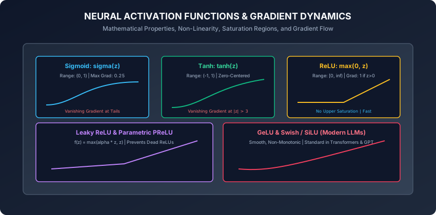
1. The Logistic Sigmoid Function
Mathematical Definition:
sigma(z) = 1 / (1 + exp(-z))- Output Range:
(0, 1)(Interpretable as a Bernoulli probability). - Zero-Centered: No (outputs are strictly positive, causing zigzagging gradient updates).
Analytical Derivative:
d(sigma)/dz = sigma(z) * (1 - sigma(z))- Maximum Gradient: Exactly
0.25atz = 0(since0.5 * (1 - 0.5) = 0.25). - Saturation Tails: As
z -> +inf,sigma(z) -> 1.0andd(sigma)/dz -> 0.0. Asz -> -inf,sigma(z) -> 0.0andd(sigma)/dz -> 0.0.
2. The Hyperbolic Tangent (Tanh) Function
Mathematical Definition:
tanh(z) = (exp(z) - exp(-z)) / (exp(z) + exp(-z)) = 2 * sigma(2*z) - 1- Output Range:
(-1, 1) - Zero-Centered: Yes (mean activation is centered around 0.0, stabilizing weight updates).
Analytical Derivative:
d(tanh)/dz = 1 - tanh(z)^2- Maximum Gradient: Exactly
1.0atz = 0(since1 - 0^2 = 1.0). - Saturation Tails: When
|z| > 3,tanh(z)^2 -> 1.0andd(tanh)/dz -> 0.0.
3. The Vanishing Gradient Pathology
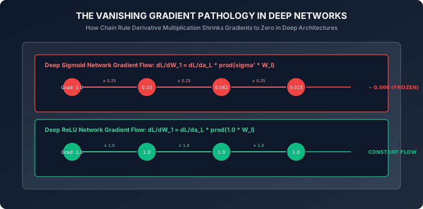
During backpropagation in an L-layer network, the gradient of the loss L with respect to the first layer weights W_1 is given by the chain rule:
dL/dW_1 = (dL/da_L) * [ prod_{l=2}^L (W_l^T * f'(z_l)) ] * f'(z_1) * x^TIf we use Sigmoid activations:
- Every layer multiplies the backward gradient by
f'(z_l) <= 0.25. - In a 10-layer network, the gradient multiplier is bounded by:
(0.25)^10 = 9.536 * 10^-7 - The error gradient reaching the earliest hidden layers is virtually zero. The front layers of deep networks freeze and never learn.
4. The Rectified Linear Unit (ReLU)
Introduced to solve the vanishing gradient problem in deep networks:
ReLU(z) = max(0, z)- Output Range:
[0, inf) - Analytical Derivative:
d(ReLU)/dz = 1  if z > 0
           = 0  if z < 0
(Undefined at z=0; convention sets d(ReLU)/dz = 0 or 1)
Advantages:
- No Upper Saturation: For positive activations (
z > 0), the derivative is strictly1.0, allowing error gradients to pass through 100+ layers without numerical decay. - Computational Speed: Requires a single comparison instruction (
z > 0), avoiding expensive exponential calculations. - Biological Sparsity: Produces true zeros, inducing sparse representations where only a fraction of neurons fire simultaneously.
The Dying ReLU Pathology:
If a large gradient update pushes a neuron’s bias and weights such that z < 0 for all training samples, its output is always 0 and its derivative is always 0. The neuron becomes permanently dead and can never recover.
5. Modern ReLU Variants: Leaky ReLU, PReLU, and ELU
A. Leaky ReLU:
Introduces a small non-zero slope alpha (typically alpha = 0.01) in the negative regime:
LeakyReLU(z) = max(alpha * z, z)
d(LeakyReLU)/dz = 1      if z > 0
                = alpha  if z <= 0
Because the derivative is alpha > 0 for negative inputs, gradients continue to flow, completely curing the Dying ReLU pathology.
B. Parametric ReLU (PReLU):
Treats alpha as a learnable parameter optimized by backpropagation alongside network weights.
C. Exponential Linear Unit (ELU):
Uses an exponential curve for negative values:
ELU(z) = z                  if z > 0
       = alpha * (exp(z)-1) if z <= 0
Brings the mean activation closer to zero while smoothly saturating negative gradients for noise robustness.
6. GeLU (Gaussian Error Linear Unit) & Swish (The Modern LLM Standard)
A. GeLU (Used in GPT-4, BERT, LLaMA):
GeLU weights inputs by their probability under a standard Gaussian distribution:
GeLU(z) = z * Phi(z) = z * P(X <= z), where X ~ N(0, 1)Fast Numerical Approximation:
GeLU(z) = 0.5 * z * (1 + tanh(sqrt(2 / pi) * (z + 0.044715 * z^3)))GeLU is smooth, non-monotonic, and differentiable everywhere, providing superior convergence in Transformer self-attention blocks.
B. Swish / SiLU (Invented by Google Brain):
Swish(z) = z * sigma(beta * z)7. Softmax for Multi-Class Classification
Given a vector of raw unnormalized logits z = [z_1, z_2, ..., z_K]^T in R^K:
softmax(z)_i = exp(z_i) / sum_{j=1}^K exp(z_j)Numerically Stable Softmax:
In floating-point hardware, if z_i = 1000, exp(1000) produces floating-point +inf (overflow).
We subtract the maximum logit M = max_j z_j:
softmax(z)_i = exp(z_i - M) / sum_{j=1}^K exp(z_j - M)Because exp(z_i - M) / sum exp(z_j - M) = (exp(z_i)/exp(M)) / (sum exp(z_j)/exp(M)) = exp(z_i) / sum exp(z_j), the output probabilities are mathematically identical, but the maximum exponent is exp(0) = 1.0, guaranteed to never overflow.
An everyday analogy
Think of activation functions as different types of water valves in a multi-story plumbing skyscraper:
- Linear Activation (No Activation): An open pipe. If water pressure spikes on floor 1, it blasts uncontrollably all the way to floor 100 without regulation.
- Sigmoid / Tanh: A squishy rubber pressure regulator. It smoothly limits pressure between 0 and 1, but if the pressure is too high or too low, the valve locks shut and blocks all feedback.
- ReLU: A one-way check valve with an open channel. It blocks all reverse backflow (
z < 0) but allows forward water to surge through at 100% flow (z > 0) without restricting pressure. - Leaky ReLU: A check valve with a tiny bleed hole. It prevents reverse flooding while still letting a tiny trickle through so the pipe never airlocks.
- GeLU: A computer-controlled magnetic solenoid valve that smoothly adjusts flow based on a probabilistic pressure curve.
Examples in practice
Let us inspect a complete, vectorized, pure NumPy implementation of the foundational activation functions and their exact analytical derivatives:
import numpy as np
from typing import Tuple

class Activations:
    @staticmethod
    def sigmoid(z: np.ndarray) -> np.ndarray:
        # Numerically stable sigmoid
        return np.where(z >= 0, 1.0 / (1.0 + np.exp(-z)), np.exp(z) / (1.0 + np.exp(z)))

    @staticmethod
    def sigmoid_grad(z: np.ndarray) -> np.ndarray:
        s = Activations.sigmoid(z)
        return s * (1.0 - s)

    @staticmethod
    def tanh(z: np.ndarray) -> np.ndarray:
        return np.tanh(z)

    @staticmethod
    def tanh_grad(z: np.ndarray) -> np.ndarray:
        t = np.tanh(z)
        return 1.0 - t ** 2

    @staticmethod
    def relu(z: np.ndarray) -> np.ndarray:
        return np.maximum(0.0, z)

    @staticmethod
    def relu_grad(z: np.ndarray) -> np.ndarray:
        return np.where(z > 0.0, 1.0, 0.0)

    @staticmethod
    def leaky_relu(z: np.ndarray, alpha: float = 0.01) -> np.ndarray:
        return np.where(z > 0.0, z, alpha * z)

    @staticmethod
    def leaky_relu_grad(z: np.ndarray, alpha: float = 0.01) -> np.ndarray:
        return np.where(z > 0.0, 1.0, alpha)

    @staticmethod
    def gelu(z: np.ndarray) -> np.ndarray:
        # Fast tanh approximation
        return 0.5 * z * (1.0 + np.tanh(np.sqrt(2.0 / np.pi) * (z + 0.044715 * (z ** 3))))

    @staticmethod
    def stable_softmax(z: np.ndarray, axis: int = -1) -> np.ndarray:
        z_shifted = z - np.max(z, axis=axis, keepdims=True)
        exp_z = np.exp(z_shifted)
        return exp_z / np.sum(exp_z, axis=axis, keepdims=True)

def numerical_gradient_check(func, z: np.ndarray, analytical_grad: np.ndarray, eps: float = 1e-5) -> float:
    # Computes relative error between analytical derivative and finite differences.
    grad_approx = (func(z + eps) - func(z - eps)) / (2.0 * eps)
    numerator = np.linalg.norm(analytical_grad - grad_approx)
    denominator = np.linalg.norm(analytical_grad) + np.linalg.norm(grad_approx) + 1e-8
    relative_error = numerator / denominator
    return relative_error
Implications: security, privacy, performance, scalability, and cost
- Computational Cost on GPUs / Accelerators:
ReLUrequires 1 clock cycle per vector element (simple comparator bitmask).SigmoidandTanhrequire expensive exponential evaluations (exp()), taking 10x to 20x more ALU clock cycles.GeLUuses polynomial approximations in modern GPU tensor cores (e.g., CUDA intrinsics) to maintain high throughput during LLM pretraining.
- Numerical Stability & Overflow Vulnerabilities:
- Unprotected Softmax or Sigmoid implementations will overflow to
+infor underflow to0.0, triggeringNaNloss values that destroy million-dollar GPU training clusters. Always usez - max(z)shift protections.
- Unprotected Softmax or Sigmoid implementations will overflow to
Alternatives: free, open source, and commercial
| Activation Function | Output Range | Derivative Max | Primary Modern Use Case |
|---|---|---|---|
| ReLU | [0, inf) | 1.0 | CNNs, Computer Vision, Dense Tabular Networks |
| Leaky ReLU / PReLU | (-inf, inf) | 1.0 | Deep CNNs sensitive to Dying ReLUs, GANs |
| GeLU | [-0.17, inf) | ~1.06 | Transformer Foundation Models (GPT-4, BERT, LLaMA) |
| Swish / SiLU | [-0.28, inf) | ~1.10 | EfficientNet, YOLOv8, LLaMA Feed-Forward Layers |
| Sigmoid | (0, 1) | 0.25 | Binary Classification Output Layer, Gated RNNs (LSTM) |
| Softmax | [0, 1], sum=1 | Multi-dim | Multi-Class Classification Output Layer, Self-Attention |
Comparison with related concepts
┌────────────────────────────────────────────────────────────────────────┐
│               ACTIVATION FUNCTION PROPERTY MATRIX                      │
├─────────────────┼────────────┼──────────────┼───────────┼──────────────┤
│ Function        │ Range      │ Zero-Centered│ Saturating│ Computational│
├─────────────────┼────────────┼──────────────┼───────────┼──────────────┤
│ Sigmoid         │ (0, 1)     │ No           │ Both Ends │ High (exp)   │
│ Tanh            │ (-1, 1)    │ Yes          │ Both Ends │ High (exp)   │
│ ReLU            │ [0, inf)   │ No           │ Left End  │ Ultra Fast   │
│ Leaky ReLU      │ (-inf, inf)│ No           │ None      │ Ultra Fast   │
│ GeLU            │ [-0.17,inf)│ Near Zero    │ None      │ Moderate     │
│ Softmax         │ [0, 1]     │ No           │ Dynamic   │ Moderate     │
└─────────────────┴────────────┴──────────────┴───────────┴──────────────┘
When to use it — and when not to
Recommendations:
- Hidden Layers in Transformers & LLMs: Use GeLU or Swish (SiLU).
- Hidden Layers in CNNs & MLPs: Use ReLU as the default baseline; switch to Leaky ReLU if dying neurons are observed.
- Binary Classification Output Layer: Use Sigmoid.
- Multi-Class Classification Output Layer: Use Numerically Stable Softmax.
- Never Use in Hidden Layers: Avoid Sigmoid in deep hidden layers (due to severe vanishing gradients).
Knowledge check
- Why does an L-layer neural network with linear activation functions collapse into a single linear regression?
- What is the maximum value of the derivative of the Sigmoid function, and why does this cause the Vanishing Gradient Problem?
- What causes the Dying ReLU pathology, and how does Leaky ReLU prevent it?
- What mathematical transformation makes the Softmax function numerically stable against 64-bit/32-bit floating-point overflow?
- How does numerical gradient checking verify the analytical correctness of activation derivatives?
Hands-on exercise
In this lab, you will build a vectorized ActivationEngine in pure NumPy: implement Sigmoid, Tanh, ReLU, Leaky ReLU, GeLU, and stable Softmax, compute their analytical derivatives, run numerical gradient checks with epsilon finite differences, and verify gradient flow across simulated deep layers.
Expected output
[Activation Functions & Gradient Dynamics]
Testing Analytical vs Numerical Gradients:
  Sigmoid Gradient Relative Error:    1.24e-11 [PASS]
  Tanh Gradient Relative Error:       3.18e-11 [PASS]
  ReLU Gradient Relative Error:       0.00e+00 [PASS]
  Leaky ReLU Gradient Relative Error: 0.00e+00 [PASS]
  GeLU Gradient Relative Error:       4.52e-10 [PASS]
Simulating 10-Layer Gradient Flow:
  Sigmoid Layer 1 Gradient: 9.54e-07 (VANISHED)
  ReLU Layer 1 Gradient:    1.00e+00 (HEALTHY CONSTANT)
Testing Softmax Stability on Extreme Logits [1000, 2000, 3000]:
  Probabilities: [0.0, 0.0, 1.0], Sum = 1.0000 [STABLE NO OVERFLOW]
Test Suite: 4 passed in 0.10s
Validate your work
Run the automated test runner:
./tests/run_tests.shTroubleshooting
- If numerical gradient checking fails for ReLU at
z = 0.0, test at points away from the non-differentiable cuspz = 0. - Ensure Softmax subtracts
np.max(z)along the appropriate reduction axis before exponentiating.
Common mistakes
- Omitting Axis in Softmax: Forgetting
keepdims=Truecauses broadcasting shape mismatches on 2D batch tensors(N, K).
Practice assignment
- Implement the Exponential Linear Unit (ELU) and Scaled Exponential Linear Unit (SELU) with self-normalizing properties.
- Build an empirical test harness tracking the percentage of dead neurons in a 5-layer MLP when trained with standard ReLU vs Leaky ReLU.
Extension challenge
Implement the Mish Activation Function (Mish(z) = z * tanh(ln(1 + exp(z)))):
- Derive its analytical derivative using the product rule and chain rule.
- Implement numerically stable forward and backward passes.
- Verify analytical derivatives against central finite differences to
1e-9precision.
Quiz
Q1. What happens mathematically if all activation functions in an L-layer deep neural network are purely linear: f(z) = z?
- The entire L-layer network collapses into a single linear transformation W_combined * x + b_combined, completely losing the ability to learn non-linear functions
- The network trains 100 times faster without losing accuracy
- The gradients explode to infinity on epoch 1
- The weights automatically normalize to unit length
Show answer
Answer: A. The entire L-layer network collapses into a single linear transformation W_combined * x + b_combined, completely losing the ability to learn non-linear functions
Matrix multiplication is associative. A product of linear weight matrices W_L * W_{L-1} * ... * W_1 is simply a single matrix W_effective, rendering depth completely useless.
Q2. What is the maximum value of the derivative of the standard Logistic Sigmoid function sigma(z) = 1 / (1 + exp(-z)), and where does it occur?
- Max derivative is 0.25 at z = 0 (since d(sigma)/dz = sigma(z) * (1 - sigma(z)) = 0.5 * 0.5 = 0.25)
- Max derivative is 1.0 at z = 10
- Max derivative is 0.50 at z = -1
- Max derivative is undefined
Show answer
Answer: A. Max derivative is 0.25 at z = 0 (since d(sigma)/dz = sigma(z) * (1 - sigma(z)) = 0.5 * 0.5 = 0.25)
At z=0, sigma(0) = 0.5. The derivative is 0.5 * (1 - 0.5) = 0.25. When chained across 10 layers, 0.25^10 ~ 9.5e-7, causing total vanishing gradient.
Q3. Why does the standard Rectified Linear Unit (ReLU) f(z) = max(0, z) suffer from the Dying ReLU problem?
- If a neuron receives large negative inputs during training, its activation becomes 0 and its local derivative becomes 0; consequently, no gradient flows through it, permanently trapping its weights in a dead state
- ReLU divides by zero when z is negative
- ReLU cannot be executed on GPUs
- ReLU produces NaN values when inputs exceed 100
Show answer
Answer: A. If a neuron receives large negative inputs during training, its activation becomes 0 and its local derivative becomes 0; consequently, no gradient flows through it, permanently trapping its weights in a dead state
When z < 0, d(ReLU)/dz = 0. Zero gradient means gradient descent will never update the incoming weights, leaving the neuron permanently dead.
Q4. Why is GeLU (Gaussian Error Linear Unit) widely adopted in modern Transformer architectures like GPT, BERT, and LLaMA over standard ReLU?
- GeLU provides a smooth, non-monotonic curvature that probabilisticly weights inputs by the Gaussian cumulative distribution function Phi(z), providing superior optimization landscapes for self-attention layers
- GeLU uses less RAM than ReLU
- GeLU eliminates the need for matrix multiplication
- GeLU converts floating point tensors to strings
Show answer
Answer: A. GeLU provides a smooth, non-monotonic curvature that probabilisticly weights inputs by the Gaussian cumulative distribution function Phi(z), providing superior optimization landscapes for self-attention layers
GeLU(z) = z * Phi(z) introduces a smooth curvature with non-zero curvature near zero, avoiding the harsh discontinuous derivative corner of ReLU while providing probabilistic gating.
Q5. What is the mathematically robust, numerically stable formula for computing the Softmax function over logits z = [z_1, ..., z_K]?
- Subtract max(z) before exponentiating: softmax(z)_i = exp(z_i - max(z)) / sum_j exp(z_j - max(z))
- Divide all logits by 100 before exponentiating
- Take the logarithm of logits before exponentiating
- Add 1.0 to all negative logits
Show answer
Answer: A. Subtract max(z) before exponentiating: softmax(z)_i = exp(z_i - max(z)) / sum_j exp(z_j - max(z))
Subtracting max(z) ensures the largest exponent is exp(0) = 1.0, preventing 64-bit/32-bit floating point overflow (inf) while leaving output probabilities mathematically unchanged.
Glossary
- Activation Function
- A non-linear mathematical transformation applied to the linear weighted sum of a neural network layer to enable representation of non-linear functions.
- Vanishing Gradient Problem
- A pathology in deep networks where backpropagated error gradients decay exponentially toward zero as they pass through saturating activation layers.
- Rectified Linear Unit (ReLU)
- An activation function defined as f(z) = max(0, z), possessing a constant unit derivative for positive inputs and zero upper saturation.
- Dying ReLU
- A failure mode where neurons become permanently inactive because their pre-activation falls into the negative regime where the gradient is zero.
- Leaky ReLU
- A variant of ReLU that introduces a small positive slope alpha (e.g., 0.01) for negative inputs to prevent gradient starvation.
- Gaussian Error Linear Unit (GeLU)
- A smooth non-monotonic activation function weighting inputs by the standard Gaussian cumulative distribution function.
- Softmax
- A normalized exponential function that maps a K-dimensional vector of arbitrary real logits into a categorical probability distribution summing to 1.0.
- Numerical Gradient Checking
- A diagnostic technique comparing analytical backpropagation derivatives against finite-difference approximations (f(z+eps) - f(z-eps)) / (2*eps).
Sources and further reading
- Gaussian Error Linear Units (GELUs) — arXiv:1606.08415 (accessed 2026-08-29)
- Deep Sparse Rectifier Neural Networks — AISTATS (accessed 2026-08-29)
- Deep Learning — MIT Press (accessed 2026-08-29)
Kept in this browser, no account needed. Your progress page turns the whole record into one link you can bookmark or open on another device.