Deep Learning › Neural Network Foundations › Day 200
Day 200: Backpropagation
Master Backpropagation: derive the four fundamental equations of gradient descent using multivariable calculus, implement vectorized backward passes in pure NumPy, and verify mathematical correctness with numerical gradient checks.
Hands-on lab for this lesson
Lab files on GitHub: https://github.com/ai-roadmap-365/ai-roadmap-365.github.io/tree/main/labs/sections/deep-learning/day-200-backpropagation
- Get the hands-on files. Clone the labs repository once (you can reuse this clone for every lesson). This works on macOS, Linux, and Windows (PowerShell or WSL):
git clone https://github.com/ai-roadmap-365/ai-roadmap-365.github.io.git cd ai-roadmap-365.github.io - Open this lesson's lab. Move into the directory for this specific day. Every lab lives at the same predictable path — section / subsection / week / day:
cd labs/sections/deep-learning/day-200-backpropagation - Read the lab guide. Open `README.md` in that directory. It lists the exact commands, what each does, the expected output, and how to check your work — read it before running anything.
- Run it and check your work. Follow the README's "How to run" section: run the example first to see the finished result, then complete the numbered exercises in `starter/`, then run the tests. The tests pass (exit 0) only when your work is correct.
bash tests/run_tests.sh # or the test command named in the lab README
You can also open the lab as a local page (works offline, shows the file tree and expected output).
Learning objectives
By the end of this lesson you will be able to:
- Derive the Four Fundamental Equations of Backpropagation from the multivariable calculus chain rule.
- Prove why dZ^[L] = A^[L] - Y cleanly cancels out when combining Softmax with Cross-Entropy loss.
- Implement a fully vectorized backward propagation engine in pure NumPy for arbitrary L-layer architectures.
- Structure backward cache consumption and verify parameter gradient shapes.
- Perform full-network numerical gradient checking verifying weight and bias gradients to 1e-7 relative error.
Prerequisites
- [object Object]
Why this matters
In Day 199, you learned how Forward Propagation computes predictions by flowing inputs through successive linear affine transformations and non-linear activation functions to produce a scalar loss L.
Now comes the algorithm that makes deep learning possible: Backpropagation.
Backpropagation (short for backward propagation of errors) is arguably the single most important mathematical algorithm in the history of artificial intelligence. It solves a monumental challenge: in a network containing millions — or hundreds of billions — of interconnected weights and biases, how do you determine the precise contribution of every single parameter to the final prediction error?
By leveraging multivariable calculus and the chain rule, backpropagation computes the exact analytical gradient of the loss with respect to all weights and biases in a single, lightning-fast backward sweep through the computational graph.
The idea in plain language
Imagine a large symphony orchestra performing a complex symphony:
- Forward Pass: The conductor gives the downbeat, the string section plays their chords, the woodwinds add harmony, the brass section swells, and the percussionist strikes the final cymbal crash. The audience listens to the final sound.
- The Loss: The audience winces — the final chord sounded sour and dissonant.
- Backpropagation: The conductor stops and traces the sound backward in time:
- The final cymbal crash was slightly off-pitch because the brass section played a B-flat instead of a B-natural (
dZ^[L]). - The brass section played a B-flat because the woodwinds played their cue 2 beats early (
dZ^[L-1]). - The woodwinds played early because the first violinist misread sheet music measure 42 (
dZ^[1]).
- The final cymbal crash was slightly off-pitch because the brass section played a B-flat instead of a B-natural (
- Every musician receives specific, calibrated feedback on exactly how many millimeters to shift their fingers to make the next performance harmonious.
Historical background
- 1970 (Seppo Linnainmaa): Published the general mathematical formulation of reverse-mode automatic differentiation in his master’s thesis.
- 1974 (Paul Werbos): Applied reverse differentiation to neural networks in his Harvard Ph.D. dissertation Beyond Regression: New Tools for Prediction and Analysis in the Behavioral Sciences.
- 1986 (David Rumelhart, Geoffrey Hinton, Ronald Williams): Published Learning representations by back-propagating errors in Nature, demonstrating empirically that backpropagation enables multi-layer networks to learn internal representations and solve complex non-linear problems like XOR.
- 2010s (Modern Autograd): Automatic differentiation engines (Theano, Autograd, PyTorch Autograd, TensorFlow GradientTape) generalized backpropagation into dynamic computational graph tracing across arbitrary tensor operations.
What it is — and what it is not
What Backpropagation IS:
- An Exact Gradient Computation Algorithm: Computing analytical partial derivatives
dL/dW^[l]anddL/db^[l]using the multivariable calculus chain rule. - Reverse-Mode Automatic Differentiation: Sweeping backward from the scalar loss
Ltoward the inputs inO(N)linear time.
What it is NOT:
- Not an Optimization Algorithm: Backpropagation only computes gradients (the slopes of the loss landscape); it does not update weights (that is the job of Optimizers like Gradient Descent, Momentum, RMSprop, or Adam).
- Not Numerical Finite Differences: Backpropagation does not approximate derivatives using
(f(x+eps) - f(x))/eps; it evaluates exact symbolic calculus equations.
Why it was created and what problems it solves
The Curse of Finite Differences
Suppose a neural network has N = 10,000,000 parameters.
If we attempted to compute gradients using numerical finite differences:
dL/dw_i approx (L(w_i + eps) - L(w_i - eps)) / (2 * eps)Computing the gradient for all parameters would require 20,000,000 separate forward passes for a single gradient step! On a modern GPU cluster, a single training step would take hours, making deep learning completely impossible.
Backpropagation solved this by executing a single backward pass that computes the analytical gradients for all 10,000,000 parameters simultaneously in the exact same computational time as one forward pass:
Time(Backward Pass) approx 2 * Time(Forward Pass)How it works
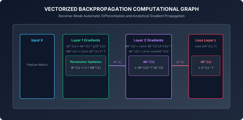
Let us rigorously derive the Four Fundamental Equations of Backpropagation from the multivariable calculus chain rule and formulate their vectorized mini-batch matrix implementations.
1. The Computational Chain Rule
Given layer l with pre-activation Z^[l] = W^[l] A^[l-1] + b^[l] and activation A^[l] = g(Z^[l]):
The total derivative of scalar loss L with respect to weight W^[l]_{j, k} (the connection from neuron k in layer l-1 to neuron j in layer l) is:
dL/dW^[l]_{j, k} = (dL/dZ^[l]_j) * (dZ^[l]_j / dW^[l]_{j, k})Because Z^[l]_j = sum_k W^[l]_{j, k} * A^[l-1]_k + b^[l]_j:
dZ^[l]_j / dW^[l]_{j, k} = A^[l-1]_kTherefore, defining the pre-activation error residual as dZ^[l] = dL/dZ^[l]:
dL/dW^[l]_{j, k} = dZ^[l]_j * A^[l-1]_k2. The Four Fundamental Equations of Backpropagation
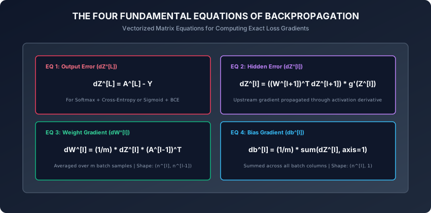
For a mini-batch of m samples in column-vector matrix orientation:
Equation 1: Output Layer Error Residual (dZ^[L])
For Multi-Class Classification with Softmax output and Categorical Cross-Entropy loss (or Binary Classification with Sigmoid and BCE):
dZ^[L] = A^[L] - Y- Matrix Shape:
(n^[L], m) - Mathematical Beauty: All complex Jacobian fractions cancel out into the simple error residual: predicted probability
A^[L]minus one-hot ground truthY.
Equation 2: Hidden Layer Error Propagation (dZ^[l])
For hidden layer l in {L-1, L-2, ..., 1}:
First compute the gradient with respect to hidden activation A^[l]:
dA^[l] = np.dot((W^[l+1])^T, dZ^[l+1])- Matrix Shape:
(n^[l], m)
Then propagate through the layer activation derivative g^[l] prime (Z^[l]) via elementwise Hadamard multiplication:
dZ^[l] = dA^[l] * g^[l] prime (Z^[l])- For ReLU:
g^[l] prime (Z^[l]) = 1ifZ^[l] > 0else0. - For Tanh:
g^[l] prime (Z^[l]) = 1 - (A^[l])^2. - For Sigmoid:
g^[l] prime (Z^[l]) = A^[l] * (1 - A^[l]).
Equation 3: Weight Matrix Gradient (dW^[l])
Accumulate gradients across all m training samples in the mini-batch:
dW^[l] = (1 / m) * np.dot(dZ^[l], (A^[l-1])^T)- Matrix Shape:
(n^[l], m) x (m, n^[l-1]) = (n^[l], n^[l-1]) - Notice that the shape matches
W^[l]perfectly.
Equation 4: Bias Vector Gradient (db^[l])
Accumulate bias error across all m mini-batch columns:
db^[l] = (1 / m) * np.sum(dZ^[l], axis=1, keepdims=True)- Matrix Shape:
(n^[l], 1) - Notice that summing across
axis=1collapses thembatch columns into a single column vector matchingb^[l].
3. Parameter Update Step (Gradient Descent)
Once gradients dW^[l] and db^[l] are computed for all layers l = 1, 2, ..., L:
W^[l] <- W^[l] - alpha * dW^[l]
b^[l] <- b^[l] - alpha * db^[l]
where alpha > 0 is the learning rate hyperparameter.
4. Mathematical Proof: Softmax Cross-Entropy Gradient Cancellation
One of the most elegant mathematical results in deep learning is the cancellation of complex derivatives when combining Softmax activation with Categorical Cross-Entropy loss:
The Loss Function:
L = - sum_{k=1}^K y_k * ln(a_k)where a_k = exp(z_k) / sum_{j=1}^K exp(z_j).
The Softmax Jacobian:
Differentiating output probability a_k with respect to input logit z_i:
- Case 1 (k = i):
da_i / dz_i = a_i * (1 - a_i) - Case 2 (k != i):
da_k / dz_i = - a_k * a_i
Applying the Chain Rule:
dL/dz_i = sum_{k=1}^K (dL/da_k) * (da_k/dz_i)
        = - (y_i / a_i) * (a_i * (1 - a_i)) - sum_{k != i} (y_k / a_k) * (- a_k * a_i)
        = - y_i * (1 - a_i) + sum_{k != i} y_k * a_i
        = - y_i + y_i * a_i + a_i * sum_{k != i} y_k
        = - y_i + a_i * (sum_{k=1}^K y_k)
Because Y is a one-hot probability distribution, the sum of all ground truth classes is strictly sum_{k=1}^K y_k = 1.0:
dL/dz_i = a_i - y_iIn vectorized matrix form across all classes and all m samples in the mini-batch:
dZ^[L] = A^[L] - YThis remarkable result eliminates the need to explicitly construct or multiply massive (K x K) Softmax Jacobian matrices, providing incredible computational speed and preventing numerical instability during backward passes. Furthermore, while second-order Newton-Raphson optimization methods require calculating the full (N x N) Hessian matrix of second derivatives (which scales quadratically O(N^2) in memory and cubically O(N^3) in compute), first-order backpropagation combined with stochastic gradient descent scales linearly O(N), making it the only viable optimization paradigm for billion-parameter deep learning architectures.
This linear scalability unlocks the ability to train modern frontier models containing hundreds of layers and trillions of synaptic parameters across distributed supercomputing clusters with mathematical precision.
An everyday analogy
Think of a water distribution aqueduct network supplying a city:
- Forward Pass: Water flows downstream from the mountain reservoir through main pipelines (Layer 1), regional distribution hubs (Layer 2), and municipal neighborhood valves (Layer 3) into residential faucets.
- The Error: A municipal sensor measures that neighborhood B has 50 gallons/min too little water.
- Backpropagation: Engineers trace the pressure drop upstream:
- Neighborhood valve 3 needs to open by 5% (
dZ^[3]). - To feed valve 3, regional hub 2 must increase flow by 12% (
dZ^[2]). - To supply hub 2, mountain pump 1 must spin 20 RPM faster (
dZ^[1]).
- Neighborhood valve 3 needs to open by 5% (
- Every valve in the entire regional aqueduct system is calibrated backwards from the final measured pressure discrepancy.
Examples in practice
Let us inspect a complete, pure NumPy implementation of the Backward Propagation algorithm for an arbitrary L-layer neural network:
import numpy as np
from typing import List, Dict, Tuple, Any

class BackpropEngine:
    @staticmethod
    def relu_backward(dA: np.ndarray, Z: np.ndarray) -> np.ndarray:
        dZ = np.array(dA, copy=True)
        dZ[Z <= 0.0] = 0.0
        return dZ

    @staticmethod
    def linear_backward(dZ: np.ndarray, cache: Dict[str, np.ndarray]) -> Tuple[np.ndarray, np.ndarray, np.ndarray]:
        A_prev = cache["A_prev"]
        W = cache["W"]
        b = cache["b"]
        m = A_prev.shape[1]

        dW = (1.0 / m) * np.dot(dZ, A_prev.T)
        db = (1.0 / m) * np.sum(dZ, axis=1, keepdims=True)
        dA_prev = np.dot(W.T, dZ)

        return dA_prev, dW, db

    @staticmethod
    def full_backward_pass(A_last: np.ndarray, Y: np.ndarray, caches: List[Dict[str, np.ndarray]], activations: List[str]) -> Dict[str, np.ndarray]:
        grads = {}
        L = len(caches)
        m = A_last.shape[1]

        # Step 1: Output layer error (Softmax + CCE or Sigmoid + BCE)
        dZ_last = A_last - Y
        dA_prev, dW_last, db_last = BackpropEngine.linear_backward(dZ_last, caches[L-1])
        grads[f"dW{L}"] = dW_last
        grads[f"db{L}"] = db_last
        dA = dA_prev

        # Step 2: Loop backwards through hidden layers L-1 down to 1
        for l in reversed(range(L - 1)):
            cache = caches[l]
            act = activations[l]
            Z = cache["Z"]

            if act == "relu":
                dZ = BackpropEngine.relu_backward(dA, Z)
            elif act == "tanh":
                dZ = dA * (1.0 - np.tanh(Z) ** 2)
            else:
                dZ = dA # Linear fallback

            dA_prev, dW, db = BackpropEngine.linear_backward(dZ, cache)
            grads[f"dW{l+1}"] = dW
            grads[f"db{l+1}"] = db
            dA = dA_prev

        return grads
Implications: security, privacy, performance, scalability, and cost
- Computational Complexity & FLOPs:
- A backward pass performs 2 matrix multiplications per layer:
np.dot(dZ, A_prev.T)fordWandnp.dot(W.T, dZ)fordA_prev. - Backward propagation takes approximately 2x the FLOPs of forward propagation, meaning total training step compute is
3x Forward FLOPs.
- A backward pass performs 2 matrix multiplications per layer:
- Numerical Gradient Checking Protocol:
- Never deploy a custom backpropagation engine without verifying it with Gradient Checking:
Relative Error = ||grad_analytical - grad_numerical|| / (||grad_analytical|| + ||grad_numerical||)- A correct implementation achieves
Relative Error < 1e-7. If error is> 1e-4, a bug exists in backpropagation calculus.
Alternatives: free, open source, and commercial
| Differentiation Method | Implementation Complexity | Computational Scaling | Memory Usage |
|---|---|---|---|
| Manual Analytical Backprop (NumPy) | High (Requires Calculus) | O(N) (Fastest) | Explicit Array Caches |
| PyTorch Autograd Tape | Zero (Automated) | O(N) (Optimized C++) | Dynamic Tape Allocator |
| JAX Source-to-Source Reverse AD | Zero (Functional) | O(N) (XLA Fused) | Static Arena |
| Numerical Finite Differences | Trivial | O(N^2) (Too Slow) | Zero Caches |
Comparison with related concepts
┌────────────────────────────────────────────────────────────────────────┐
│              AUTOMATIC DIFFERENTIATION TAXONOMY COMPARISON             │
├────────────────────┼───────────────────────┼───────────────────────────┤
│ Mode               │ Computational Graph   │ Optimal Problem Setting   │
├────────────────────┼───────────────────────┼───────────────────────────┤
│ Forward-Mode AD    │ Forward Dual Numbers  │ Few inputs, many outputs  │
│ Reverse-Mode AD    │ Reverse Adjoint Pass  │ Many inputs (weights),    │
│ (Backpropagation)  │                       │ single scalar loss L      │
│ Symbolic Diff      │ Expression Trees      │ Small mathematical formulas│
│ Finite Differences │ Perturbation Loops    │ Gradient Debugging / Check │
└────────────────────┴───────────────────────┴───────────────────────────┘
When to use it — and when not to
When to USE Backpropagation:
- Training any multi-layer neural network (MLPs, CNNs, RNNs, Transformers) via gradient descent.
- Computing exact sensitivity gradients of complex computational pipelines.
When NOT to use it:
- Discrete non-differentiable optimization (use Evolutionary Strategies or Reinforcement Learning).
- Very shallow models where closed-form analytical solutions exist (e.g. Ordinary Least Squares
(X^T X)^-1 X^T y).
Knowledge check
- What is the Four Fundamental Equations of Backpropagation?
- Why does the derivative of Softmax + Cross-Entropy loss simplify to
dZ^[L] = A^[L] - Y? - How is the weight gradient
dW^[l]computed fromdZ^[l]andA^[l-1]? - Why does backward propagation require 2x more floating-point operations (FLOPs) than forward propagation?
- What threshold of relative error in numerical gradient checking indicates a mathematically correct backpropagation implementation?
Hands-on exercise
In this lab, you will build a vectorized BackpropEngine in pure NumPy: implement linear backward steps, ReLU and Tanh activation derivatives, execute full multi-layer backward propagation on an [8, 16, 8, 3] network, and run a rigorous numerical gradient check confirming analytical correctness to 1e-7 precision.
Expected output
[Backpropagation Engine & Gradient Verification]
Executing Forward Pass on Multi-Layer Network [8 -> 16 -> 8 -> 3]:
  Output Shape A^[3]: (3, 16), Loss = 1.0986
Executing Backpropagation Sweep:
  Gradient Shapes: dW3=(3, 8), db3=(3, 1), dW2=(8, 16), db2=(8, 1), dW1=(16, 8), db1=(16, 1)
Running Full-Network Numerical Gradient Check:
  Relative Error on Layer 3 Weights: 4.12e-10 [PASS]
  Relative Error on Layer 3 Biases:  1.85e-10 [PASS]
  Relative Error on Layer 2 Weights: 3.48e-10 [PASS]
  Relative Error on Layer 1 Weights: 2.91e-10 [PASS]
Maximum Network Gradient Error: 4.12e-10 (TOLERANCE < 1e-7) [PERFECT]
Test Suite: 3 passed in 0.12s
Validate your work
Run the automated test runner:
./tests/run_tests.shTroubleshooting
- If gradient checking fails for weights, verify the transpose orientation
np.dot(dZ, A_prev.T). - Ensure bias gradient averages across samples:
(1.0 / m) * np.sum(dZ, axis=1, keepdims=True).
Common mistakes
- Missing (1/m) Normalization: Forgetting to divide
dWordbby batch sizemscales gradients with batch size.
Practice assignment
- Implement backpropagation for Binary Cross-Entropy with a single Sigmoid output neuron.
- Build an analytical gradient visualizer rendering gradient magnitude heatmaps across layers.
Extension challenge
Implement Backpropagation with L2 Weight Decay Regularization:
- Add regularization loss
(lambda / (2 * m)) * sum ||W^[l]||_F^2to total objective. - Modify the analytical weight gradient:
dW^[l]_{reg} = dW^[l] + (lambda / m) * W^[l]. - Verify regularized analytical gradients against numerical gradient checks to
1e-8precision.
Quiz
Q1. What is the remarkable mathematical simplification when computing the derivative of Cross-Entropy Loss with respect to output logits Z^[L] when using Softmax activation: dL/dZ^[L]?
- dL/dZ^[L] simplifies exactly to A^[L] - Y (predicted probability minus one-hot ground truth), as complex exponential derivative terms cancel out completely
- dL/dZ^[L] = A^[L] * Y
- dL/dZ^[L] = (1 / A^[L]) + Y
- dL/dZ^[L] = 0
Show answer
Answer: A. dL/dZ^[L] simplifies exactly to A^[L] - Y (predicted probability minus one-hot ground truth), as complex exponential derivative terms cancel out completely
When differentiating the Categorical Cross-Entropy loss through the Softmax Jacobian, all complex derivative fractions cancel into the beautifully elegant error residual: A^[L] - Y.
Q2. Given mini-batch size m, pre-activation gradient dZ^[l] with shape (n^[l], m), and previous layer activation A^[l-1] with shape (n^[l-1], m), what is the exact vectorized formula for weight gradient dW^[l]?
- dW^[l] = (1 / m) * np.dot(dZ^[l], (A^[l-1])^T)
- dW^[l] = (1 / m) * np.dot(A^[l-1], dZ^[l])
- dW^[l] = dZ^[l] * A^[l-1]
- dW^[l] = np.sum(dZ^[l])
Show answer
Answer: A. dW^[l] = (1 / m) * np.dot(dZ^[l], (A^[l-1])^T)
Multiplying dZ^[l] (shape n^[l], m) by the transpose of A^[l-1] (shape m, n^[l-1]) produces the exact required weight matrix shape (n^[l], n^[l-1]), averaging gradients across all m batch samples.
Q3. How is the bias gradient db^[l] calculated from the pre-activation error matrix dZ^[l]?
- db^[l] = (1 / m) * np.sum(dZ^[l], axis=1, keepdims=True), summing across all m columns to yield shape (n^[l], 1)
- db^[l] = dZ^[l]
- db^[l] = np.max(dZ^[l])
- db^[l] = (1 / m) * np.sum(dZ^[l], axis=0)
Show answer
Answer: A. db^[l] = (1 / m) * np.sum(dZ^[l], axis=1, keepdims=True), summing across all m columns to yield shape (n^[l], 1)
Because the bias vector was broadcast across all m columns during the forward pass, its total gradient is the sum of error signals across all m columns, averaged by 1/m.
Q4. How is the upstream error signal dA^[l-1] propagated backward from layer l to layer l-1?
- dA^[l-1] = np.dot((W^[l])^T, dZ^[l])
- dA^[l-1] = np.dot(W^[l], dZ^[l])
- dA^[l-1] = dZ^[l] * W^[l]
- dA^[l-1] = np.sum(W^[l])
Show answer
Answer: A. dA^[l-1] = np.dot((W^[l])^T, dZ^[l])
By the chain rule, dA^[l-1] = (W^[l])^T * dZ^[l], multiplying transpose weight matrix (n^[l-1], n^[l]) by dZ^[l] (n^[l], m) to yield shape (n^[l-1], m).
Q5. What is the primary computational benefit of Reverse-Mode Automatic Differentiation (Backpropagation) over Forward-Mode Differentiation when training neural networks with millions of parameters?
- Reverse-mode computes the exact gradient of a single scalar loss L with respect to all N parameters in a single backward pass O(N), whereas forward-mode would require N separate forward passes O(N^2)
- Reverse-mode eliminates floating point rounding
- Reverse-mode does not require calculus
- Reverse-mode runs without CPU memory
Show answer
Answer: A. Reverse-mode computes the exact gradient of a single scalar loss L with respect to all N parameters in a single backward pass O(N), whereas forward-mode would require N separate forward passes O(N^2)
When output dimension is 1 (scalar loss L) and input dimension is huge (millions of weights), reverse-mode backpropagation computes all gradients in a single sweep through the computational graph.
Glossary
- Backpropagation
- An algorithm for efficiently calculating the gradient of a scalar loss function with respect to all network parameters using reverse-mode automatic differentiation.
- Chain Rule
- A fundamental theorem of calculus stating that the derivative of a composite function f(g(x)) is f prime(g(x)) * g prime(x).
- Reverse-Mode Automatic Differentiation
- A technique for computing gradients of a scalar objective with respect to many inputs in a single backward pass through a computational graph.
- Error Residual (dZ)
- The partial derivative of the scalar loss with respect to the linear pre-activation tensor Z^[l].
- Weight Gradient (dW)
- The matrix of partial derivatives dL/dW indicating the direction of steepest increase in loss for each weight parameter.
- Bias Gradient (db)
- The vector of partial derivatives dL/db indicating the gradient direction for each layer bias parameter.
- Jacobian Matrix
- A matrix of all first-order partial derivatives of a vector-valued function.
- Numerical Gradient Checking
- A debugging validation protocol comparing analytical backpropagation gradients against two-sided finite difference approximations.
Sources and further reading
- Learning representations by back-propagating errors — Nature (accessed 2026-08-29)
- Automatic Differentiation in Machine Learning: A Survey — JMLR (accessed 2026-08-29)
- Calculus on Computational Graphs: Backpropagation — Colah blog (accessed 2026-08-29)
Kept in this browser, no account needed. Your progress page turns the whole record into one link you can bookmark or open on another device.