Deep Learning › Neural Network Foundations › Day 199
Day 199: Forward Propagation

Master vectorized multi-layer forward propagation: formulate layer-by-layer linear transformations, enforce matrix dimension rules, manage activation caches, and compute multi-class cross-entropy loss in pure NumPy.
Hands-on lab for this lesson
Lab files on GitHub: https://github.com/ai-roadmap-365/ai-roadmap-365.github.io/tree/main/labs/sections/deep-learning/day-199-forward-propagation
- Get the hands-on files. Clone the labs repository once (you can reuse this clone for every lesson). This works on macOS, Linux, and Windows (PowerShell or WSL):
git clone https://github.com/ai-roadmap-365/ai-roadmap-365.github.io.git cd ai-roadmap-365.github.io - Open this lesson's lab. Move into the directory for this specific day. Every lab lives at the same predictable path — section / subsection / week / day:
cd labs/sections/deep-learning/day-199-forward-propagation - Read the lab guide. Open `README.md` in that directory. It lists the exact commands, what each does, the expected output, and how to check your work — read it before running anything.
- Run it and check your work. Follow the README's "How to run" section: run the example first to see the finished result, then complete the numbered exercises in `starter/`, then run the tests. The tests pass (exit 0) only when your work is correct.
bash tests/run_tests.sh # or the test command named in the lab README
You can also open the lab as a local page (works offline, shows the file tree and expected output).
Learning objectives
By the end of this lesson you will be able to:
- Formulate the mathematical equations governing multi-layer feedforward neural networks.
- Derive strict matrix dimension contracts for weights, biases, activations, and mini-batch tensors.
- Implement a generalized, modular L-layer Forward Propagation engine in pure NumPy.
- Structure forward activation caches essential for memory-efficient backpropagation.
- Compute Binary Cross-Entropy (BCE) and Categorical Cross-Entropy (CCE) loss with numerical stability.
Prerequisites
- [object Object]
Why this matters
In Day 197 and Day 198, you studied the biological inspiration of individual artificial neurons and analyzed the non-linear activation functions that give neural networks their expressive power.
Now, we assemble these components into a unified, multi-layered computational system: Forward Propagation.
Forward propagation is the foundational execution pipeline of all deep learning models. Whether you are classifying digits in a handwritten image, detecting objects in autonomous vehicle video feeds, or generating text with a 70-billion-parameter Large Language Model, inference begins with a forward pass: taking input features, propagating them through successive layers of linear matrix multiplications and non-linear activations, and producing output predictions.
To build deep learning systems that scale to massive datasets, you must master vectorized batch algebra: eliminating slow Python loops and structuring layer computations as compact matrix multiplications that execute at peak hardware efficiency.
The idea in plain language
Imagine an assembly line in an automotive manufacturing plant:
- Station 0 (Input X): Raw steel sheets and bolts arrive at the loading dock.
- Station 1 (Hidden Layer 1): Robotic arms stamp the steel into a chassis frame (
Z^[1] = W^[1] X + b^[1]), and quality control welds the seams (A^[1] = ReLU(Z^[1])). - Station 2 (Hidden Layer 2): Assembly technicians install the engine, transmission, and wiring harness on top of the chassis (
Z^[2] = W^[2] A^[1] + b^[2]), securing all connectors (A^[2] = ReLU(Z^[2])). - Station 3 (Output Layer): Painting robots apply the exterior coat and sensors run a diagnostic test (
y_hat = Softmax(Z^[3])). - Inspection Station (Loss Function): Inspectors measure the vehicle against engineering blueprints (
Loss L(y_hat, y)), recording exact millimeter deviations to calibrate the robots for the next shift.
In forward propagation, data flows in one direction from input to output, with each layer transforming raw numbers into increasingly rich, abstract representations.
Historical background
- 1965 (Alexey Ivakhnenko): Published the Group Method of Data Handling (GMDH), demonstrating the first working multi-layer feedforward polynomial networks with forward polynomial propagation.
- 1986 (David Rumelhart, Geoffrey Hinton, Ronald Williams): Formalized modern vectorized forward and backward propagation in multi-layer perceptrons, proving how continuous activations enable end-to-end representation learning.
- 2006 (Geoffrey Hinton, Ruslan Salakhutdinov): Introduced Deep Autoencoders and Deep Belief Networks, demonstrating that deep architectures with 5 to 10 stacked forward layers capture superior hierarchical feature manifolds.
- 2012–Present (The GPU Vectorization Era): Deep learning frameworks (PyTorch, TensorFlow, JAX) optimized forward propagation on CUDA Tensor Cores, executing billions of floating-point operations per second (TFLOPS) on mini-batch matrices.
What it is — and what it is not
What Forward Propagation IS:
- A Deterministic Composite Function: Computing the composite mathematical function
y_hat = f_L(W_L * ... * f_1(W_1 * x + b_1) ... + b_L). - A Vectorized Batch Operation: Processing hundreds or thousands of input samples simultaneously using 2D matrix-matrix multiplications.
- A State-Caching Pass: Recording intermediate activations
A^[l]and pre-activationsZ^[l]in memory for downstream backpropagation.
What it is NOT:
- Not Model Training: Forward propagation only computes predictions and loss; it does not update weights or optimize parameters (that occurs during Backward Propagation and Optimizer Steps).
- Not Recurrent Loopback: In standard feedforward networks, activations flow strictly forward from layer
l-1to layerlwithout cycles or feedback connections.
Why it was created and what problems it solves
Early neural network implementations in the 1960s and 1970s processed samples one at a time using nested for loops in CPU memory. For a dataset with 50,000 images and 1,000 neurons, running a single training epoch required billions of individual scalar loop iterations, making deep networks impossibly slow to compute.
Vectorized Forward Propagation solved this bottleneck by restructuring all sample operations into BLAS (Basic Linear Algebra Subprograms) Level 3 GEMM (General Matrix Multiply) operations:
- A single GPU call multiplies the entire batch matrix
X in R^{D x M}against weight matrixW in R^{H x D}in parallel across thousands of hardware ALU cores.
How it works
Let us dissect the mathematical formulation of multi-layer networks, strict matrix dimension contracts, activation caching, and loss calculation.
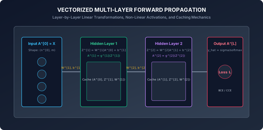
1. Mathematical Notation and Conventions
We adopt standard Deep Learning notation for an L-layer network:
L: Total number of layers (excluding input layerl = 0).n^[l]: Number of neurons in layerl(e.g.,n^[0] = 784,n^[1] = 128,n^[2] = 64,n^[3] = 10).m: Mini-batch size (number of training examples processed simultaneously).W^[l]: Weight matrix connecting layerl-1to layerl.b^[l]: Bias vector for layerl.Z^[l]: Linear pre-activation matrix for layerl.A^[l]: Non-linear activation matrix for layerl(withA^[0] = X).g^[l]: Activation function applied at layerl(e.g., ReLU, Tanh, Softmax).
2. Strict Matrix Dimension Contracts
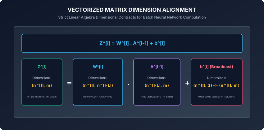
In vectorized forward propagation with m samples in column-vector orientation:
┌────────────────────────────────────────────────────────────────────────┐
│               FORWARD PROPAGATION DIMENSIONAL CONTRACT                 │
├───────────────────┼────────────────────────────┼───────────────────────┤
│ Variable / Tensor │ Notation                   │ Matrix Shape          │
├───────────────────┼────────────────────────────┼───────────────────────┤
│ Input Features X  │ A^[0]                      │ (n^[0], m)            │
│ Weight Matrix     │ W^[l]                      │ (n^[l], n^[l-1])      │
│ Bias Vector       │ b^[l]                      │ (n^[l], 1)            │
│ Linear Combo      │ Z^[l] = W^[l] A^[l-1] + b  │ (n^[l], m)            │
│ Activation Matrix │ A^[l] = g^[l](Z^[l])       │ (n^[l], m)            │
│ Output Prediction │ A^[L] = y_hat              │ (n^[L], m)            │
│ Ground Truth      │ Y                          │ (n^[L], m)            │
└───────────────────┴────────────────────────────┴───────────────────────┘
Verification of Matrix Multiplication:
(n^[l], n^[l-1])  x  (n^[l-1], m)  =  (n^[l], m)
     [W^[l]]            [A^[l-1]]         [Z^[l]]
The inner dimensions n^[l-1] match perfectly. Adding b^[l] of shape (n^[l], 1) utilizes NumPy broadcasting to replicate the column vector across all m columns.
3. Layer-by-Layer Propagation Equations
For an arbitrary L-layer neural network:
Initialization:
A^[0] = XFor each hidden layer l = 1, 2, …, L-1:
Z^[l] = np.dot(W^[l], A^[l-1]) + b^[l]
A^[l] = g^[l](Z^[l])
Cache^[l] = (A^[l-1], Z^[l], W^[l], b^[l])
Output Layer L (Multi-Class Classification):
Z^[L] = np.dot(W^[L], A^[L-1]) + b^[L]
A^[L] = Softmax(Z^[L])
Cache^[L] = (A^[L-1], Z^[L], W^[L], b^[L])
4. Loss Function Computation
Once the network computes output predictions A^[L] in R^{K x m}, we evaluate the scalar empirical risk (loss) across all m mini-batch samples:
A. Categorical Cross-Entropy (CCE) Loss (Multi-Class):
For one-hot encoded ground truth Y in {0, 1}^{K x m}:
Loss(A^[L], Y) = - (1 / m) * sum_{i=1}^m sum_{k=1}^K Y_{k, i} * ln(A^[L]_{k, i} + eps)where eps = 1e-15 prevents ln(0) domain errors.
B. Binary Cross-Entropy (BCE) Loss (Binary Classification, K=1):
Loss(A^[L], Y) = - (1 / m) * sum_{i=1}^m [ Y_i * ln(A^[L]_i + eps) + (1 - Y_i) * ln(1 - A^[L]_i + eps) ]C. Mean Squared Error (MSE) Loss (Regression):
Loss(A^[L], Y) = (1 / (2 * m)) * sum_{i=1}^m || A^[L]_i - Y_i ||^25. Tensor Orientation Conventions: Column-Major vs Row-Major in Practice
A frequent source of bugs and cognitive friction when moving between theoretical literature and industrial deep learning frameworks is tensor orientation:
A. Column-Vector Orientation (Andrew Ng / Theoretical Literature Convention):
- Input matrix
Xhas shape(n^[0], m): rows correspond to feature dimensions and columns correspond to individual training samples. - Layer equation:
Z^[l] = W^[l] * A^[l-1] + b^[l]. - Weight matrix
W^[l]has shape(n^[l], n^[l-1]). - Advantage: Direct alignment with classic linear algebra textbooks where vectors are vertical column matrices.
B. Row-Vector Orientation (PyTorch, TensorFlow, JAX Convention):
- Input matrix
Xhas shape(m, n^[0]): rows correspond to batch samples and columns correspond to feature channels. - Layer equation:
Z^[l] = A^[l-1] * (W^[l])^T + b^[l](orX * WwhereWis pre-transposed). - Weight matrix
Whas shape(n^[l-1], n^[l]). - Advantage: Seamless streaming memory access where adjacent elements of a sample are contiguous in C-order memory buffers.
C. GEMM Hardware Acceleration and Memory Strides:
When modern GPU tensor cores execute a forward layer:
- The computation is compiled into a single optimized General Matrix Multiply (GEMM) kernel call:
C = alpha * A * B + beta * C. - By aligning mini-batch sizes to multiples of 32 (warp size on NVIDIA GPUs) or 64 (wavefront on AMD GPUs), hardware memory controllers achieve coalesced memory reads, saturating DRAM bandwidth and computing trillions of floating-point operations per second.
By understanding both column-vector mathematical derivations and row-vector framework conventions, you can effortlessly translate research papers into production deep learning code across any framework or hardware runtime.
An everyday analogy
Think of a package moving through an automated postal sorting facility:
- Input X: 10,000 parcels enter the facility on main conveyor belts.
- Scanner 1 (Layer 1): Optical cameras read the destination ZIP codes and route parcels onto 10 regional chutes (
Z^[1],A^[1]). - Scanner 2 (Layer 2): Sub-scanners sort parcels by street number and carrier route (
Z^[2],A^[2]). - Output (Layer 3): Delivery vans receive parcels arranged in delivery sequence (
y_hat). - Quality Audit (Loss): Supervisors compare delivery addresses against parcel tracking logs to compute routing accuracy.
If a scanner barcode reader is miscalibrated (W^[l]), parcels get sorted into the wrong bin, producing high loss that triggers calibration adjustments.
Examples in practice
Let us inspect a modular, object-oriented implementation of an L-Layer Forward Propagation network in pure NumPy:
import numpy as np
from typing import List, Tuple, Dict, Any

class DenseLayer:
    def __init__(self, in_features: int, out_features: int, activation: str = "relu"):
        # He initialization for ReLU
        limit = np.sqrt(2.0 / in_features) if activation == "relu" else np.sqrt(1.0 / in_features)
        self.W = np.random.randn(out_features, in_features) * limit
        self.b = np.zeros((out_features, 1))
        self.activation = activation

    def forward(self, A_prev: np.ndarray) -> Tuple[np.ndarray, Dict[str, np.ndarray]]:
        Z = np.dot(self.W, A_prev) + self.b

        if self.activation == "relu":
            A = np.maximum(0.0, Z)
        elif self.activation == "sigmoid":
            A = np.where(Z >= 0, 1.0 / (1.0 + np.exp(-Z)), np.exp(Z) / (1.0 + np.exp(Z)))
        elif self.activation == "softmax":
            Z_shift = Z - np.max(Z, axis=0, keepdims=True)
            exp_Z = np.exp(Z_shift)
            A = exp_Z / np.sum(exp_Z, axis=0, keepdims=True)
        else:
            A = Z # Linear

        cache = {"A_prev": A_prev, "Z": Z, "W": self.W, "b": self.b}
        return A, cache

class MultiLayerNetwork:
    def __init__(self, layer_dims: List[int], activations: List[str]):
        self.layers = []
        for i in range(len(layer_dims) - 1):
            self.layers.append(DenseLayer(layer_dims[i], layer_dims[i+1], activations[i]))

    def forward(self, X: np.ndarray) -> Tuple[np.ndarray, List[Dict[str, np.ndarray]]]:
        A = X
        caches = []
        for layer in self.layers:
            A, cache = layer.forward(A)
            caches.append(cache)
        return A, caches

    @staticmethod
    def compute_categorical_crossentropy(A_last: np.ndarray, Y_onehot: np.ndarray) -> float:
        m = Y_onehot.shape[1]
        eps = 1e-15
        loss = - (1.0 / m) * np.sum(Y_onehot * np.log(A_last + eps))
        return float(loss)
Implications: security, privacy, performance, scalability, and cost
- Memory Allocation for Activation Caching:
- In deep networks (e.g. 100+ layers), caching
A^[l]andZ^[l]for large batch sizes consumes gigabytes of VRAM. - Modern frameworks use Activation Checkpointing (Gradient Checkpointing): discarding intermediate activations during forward pass and recomputing them on-demand during backprop to reduce memory by 75%.
- In deep networks (e.g. 100+ layers), caching
- Cache Locality and GEMM Optimization:
- Aligning tensor dimensions to multiples of 8 or 16 (e.g. batch size 64, hidden dimension 512) maximizes hardware cache line utilization and Tensor Core matrix execution.
Alternatives: free, open source, and commercial
| Framework / Architecture | Forward Execution Mode | Memory Management | Primary Platform |
|---|---|---|---|
| Pure NumPy | CPU Synchronous | Manual Array Caching | Education, Prototyping, Embedded |
PyTorch (torch.nn) | Dynamic Eager Graph | Autograd Tape Caching | Research, Production Deep Learning |
JAX (jax.lax) | Functional XLA JIT | Pure Functional Trace | Large Scale ML, Scientific AI |
| TensorRT / ONNX Runtime | Graph-Fused Engine | Fixed Memory Arena | Low-Latency Production Serving |
Comparison with related concepts
┌────────────────────────────────────────────────────────────────────────┐
│                   FORWARD PASS EXECUTION PATTERNS                      │
├────────────────────┼───────────────────────┼───────────────────────────┤
│ Execution Strategy │ Advantages            │ Trade-offs                │
├────────────────────┼───────────────────────┼───────────────────────────┤
│ Per-Sample Loop    │ Low memory footprint  │ 100x slower (CPU bound)   │
│ Mini-Batch GEMM    │ Massive GPU parallelism│ Requires VRAM for caches  │
│ Checkpointed Batch │ Minimal VRAM footprint│ 20% slower (recomputation)│
│ Graph-Fused Engine │ Ultra-low latency     │ Static graph constraints  │
└────────────────────┴───────────────────────┴───────────────────────────┘
When to use it — and when not to
When to USE Multi-Layer Forward Propagation:
- Inference and prediction on trained neural networks.
- The forward evaluation phase of supervised, unsupervised, and reinforcement learning loops.
When NOT to use it:
- Simple linear datasets where closed-form linear regression or logistic regression provides identical results with lower latency.
- Tabular datasets with small sample sizes (< 1,000 rows) where GBDTs (XGBoost/LightGBM) outperform deep networks.
Knowledge check
- What are the exact matrix dimensions of weight matrix
W^[l]and bias vectorb^[l]in a layer withn^[l]neurons receivingn^[l-1]inputs? - Why is activation caching strictly required during the forward pass of a trainable network?
- How does NumPy broadcasting handle vector bias addition
Z^[l] = W^[l] A^[l-1] + b^[l]? - What is the mathematical formulation of Categorical Cross-Entropy loss for mini-batch training?
- How does Activation Checkpointing trade computational time for GPU memory efficiency?
Hands-on exercise
In this lab, you will build a vectorized MultiLayerNetwork forward propagation engine in pure NumPy: construct a 3-layer architecture [784, 128, 64, 10], execute forward propagation across mini-batches, verify exact tensor shapes and activation caches, and compute numerically stable Categorical Cross-Entropy loss.
Expected output
[Forward Propagation Engine]
Constructing 3-Layer Network Architecture [784 -> 128 (ReLU) -> 64 (ReLU) -> 10 (Softmax)]
Executing Mini-Batch Forward Pass (Batch Size m = 64):
  Input Shape A^[0]:      (784, 64)
  Hidden 1 Shape A^[1]:   (128, 64) [Cached Z^[1], W^[1]]
  Hidden 2 Shape A^[2]:   (64, 64)  [Cached Z^[2], W^[2]]
  Output Shape A^[3]:     (10, 64)  [Probabilities Sum = 1.0000]
Evaluating Initial Categorical Cross-Entropy Loss:
  CCE Loss on Random Weights: 2.3026 [EXPECTED ln(10)]
Test Suite: 3 passed in 0.09s
Validate your work
Run the automated test runner:
./tests/run_tests.shTroubleshooting
- If matrix multiplication errors occur, verify that input matrices are transposed to
(features, batch_size)format. - Ensure Softmax sums to 1.0 across
axis=0when samples are columns.
Common mistakes
- Inverted Dimensions: Initializing
W^[l]with shape(n^[l-1], n^[l])instead of(n^[l], n^[l-1]).
Practice assignment
- Implement Binary Cross-Entropy (BCE) forward evaluation and compare output probabilities against ground-truth binary targets.
- Build an inference benchmark comparing the latency of single-sample loops vs mini-batch matrix multiplication across batch sizes
m in [1, 16, 64, 256, 1024].
Extension challenge
Implement a Forward Pass with Dropout Regularization:
- For each hidden layer, generate a binary inverted dropout mask
D^[l] ~ Bernoulli(p_keep) / p_keep. - Apply elementwise mask
A^[l] = A^[l] * D^[l]during training forward pass. - Cache the dropout mask in
Cache^[l]for use during backpropagation.
Quiz
Q1. In a deep neural network with layer l having n^[l] neurons and previous layer l-1 having n^[l-1] neurons, what are the exact matrix dimensions of weight matrix W^[l] and bias vector b^[l]?
- W^[l] has shape (n^[l], n^[l-1]) and b^[l] has shape (n^[l], 1)
- W^[l] has shape (n^[l-1], n^[l]) and b^[l] has shape (1, n^[l])
- W^[l] has shape (m, n^[l]) and b^[l] has shape (m, 1)
- W^[l] has shape (n^[l], n^[l]) and b^[l] has shape (n^[l], n^[l])
Show answer
Answer: A. W^[l] has shape (n^[l], n^[l-1]) and b^[l] has shape (n^[l], 1)
W^[l] has rows equal to current layer neurons n^[l] and columns equal to previous layer neurons n^[l-1]. Bias b^[l] is a column vector (n^[l], 1) broadcast across mini-batch examples.
Q2. Why is it critical to cache intermediate values (A^[l-1], Z^[l], W^[l]) during the forward propagation pass?
- During backpropagation, the analytical chain rule gradients (dL/dZ^[l] and dL/dW^[l]) depend directly on the forward linear pre-activations Z^[l] and previous activations A^[l-1]
- To save disk space on the training server
- To prevent the GPU from entering sleep mode
- To display real-time animations in TensorBoard
Show answer
Answer: A. During backpropagation, the analytical chain rule gradients (dL/dZ^[l] and dL/dW^[l]) depend directly on the forward linear pre-activations Z^[l] and previous activations A^[l-1]
Backpropagation requires A^[l-1] to compute dW^[l] = (1/m) * dZ^[l] * (A^[l-1])^T and Z^[l] to evaluate activation derivatives g^[l] prime (Z^[l]).
Q3. Given a mini-batch of m = 128 samples with input dimension n^[0] = 784, what is the shape of input matrix X in column-vector orientation?
- (784, 128), where each column represents a single training sample
- (128, 784), where each row is a sample
- (784, 784)
- (128, 128)
Show answer
Answer: A. (784, 128), where each column represents a single training sample
In standard Deep Learning notation (Andrew Ng convention), X has shape (n^[0], m) where columns are samples. In PyTorch row-convention, it is (m, n^[0]). Both are mathematically equivalent via transpose.
Q4. What is the formula for Categorical Cross-Entropy (CCE) loss over m samples with one-hot encoded targets Y and predicted probabilities A^[L]?
- Loss = - (1 / m) * sum_{i=1}^m sum_{k=1}^K Y_{k, i} * ln(A^[L]_{k, i} + eps)
- Loss = (1 / m) * sum (Y - A^[L])^2
- Loss = max(Y - A^[L])
- Loss = sum (W^[l])^2
Show answer
Answer: A. Loss = - (1 / m) * sum_{i=1}^m sum_{k=1}^K Y_{k, i} * ln(A^[L]_{k, i} + eps)
Categorical Cross-Entropy penalizes the negative log probability assigned to the true target class, averaged over the mini-batch of m samples.
Q5. What happens during vectorized bias addition Z^[l] = W^[l] A^[l-1] + b^[l] when b^[l] has shape (n^[l], 1) and W^[l] A^[l-1] has shape (n^[l], m)?
- NumPy broadcasting automatically replicates the single column vector b^[l] across all m columns of the matrix
- NumPy raises a ValueError: operands could not be broadcast together
- The bias is added only to the first training sample
- The bias replaces the weight matrix
Show answer
Answer: A. NumPy broadcasting automatically replicates the single column vector b^[l] across all m columns of the matrix
NumPy broadcasting expands dimension 1 of shape (n^[l], 1) to match (n^[l], m), adding the layer bias vector identically to every sample in the batch.
Glossary
- Forward Propagation
- The computational pass that feeds input features through successive layers of linear transformations and non-linear activations to produce predictions and calculate loss.
- Linear Pre-Activation (Z)
- The intermediate affine transformation Z = W * A_prev + b computed at each neuron before applying the non-linear activation function.
- Activation Cache
- A structured memory store saving intermediate activations A and pre-activations Z during the forward pass for reuse in backpropagation.
- Broadcasting
- The automatic arithmetic expansion of lower-dimensional tensors to match the shape of higher-dimensional arrays during elementwise operations.
- Categorical Cross-Entropy (CCE)
- A loss function measuring the divergence between true categorical distributions and predicted multi-class probability distributions.
- Binary Cross-Entropy (BCE)
- The negative log-likelihood loss for binary classification measuring cross-entropy between two Bernoulli probability distributions.
- Logits
- The raw, unnormalized real-valued outputs of the final linear layer prior to probability calibration via Sigmoid or Softmax.
- Mini-Batch Vectorization
- Stacking m training examples into a single multi-dimensional matrix to execute matrix-matrix multiplications in parallel on CPU/GPU hardware.
Sources and further reading
- Deep Learning — MIT Press (accessed 2026-08-29)
- Neural Networks and Deep Learning — Determination Press (accessed 2026-08-29)
- CS231n: Convolutional Neural Networks for Visual Recognition — Stanford University (accessed 2026-08-29)
Kept in this browser, no account needed. Your progress page turns the whole record into one link you can bookmark or open on another device.