Deep Learning › Neural Network Foundations › Day 203
Day 203: Training MNIST from Scratch

Train a complete two-layer neural network on the classic MNIST benchmark in pure NumPy: parse image binary tensors, implement vectorized mini-batch SGD with Momentum, reach >= 95% test accuracy, and conduct error analysis on misclassified digits.
Hands-on lab for this lesson
Lab files on GitHub: https://github.com/ai-roadmap-365/ai-roadmap-365.github.io/tree/main/labs/sections/deep-learning/day-203-training-mnist-from-scratch
- Get the hands-on files. Clone the labs repository once (you can reuse this clone for every lesson). This works on macOS, Linux, and Windows (PowerShell or WSL):
git clone https://github.com/ai-roadmap-365/ai-roadmap-365.github.io.git cd ai-roadmap-365.github.io - Open this lesson's lab. Move into the directory for this specific day. Every lab lives at the same predictable path — section / subsection / week / day:
cd labs/sections/deep-learning/day-203-training-mnist-from-scratch - Read the lab guide. Open `README.md` in that directory. It lists the exact commands, what each does, the expected output, and how to check your work — read it before running anything.
- Run it and check your work. Follow the README's "How to run" section: run the example first to see the finished result, then complete the numbered exercises in `starter/`, then run the tests. The tests pass (exit 0) only when your work is correct.
bash tests/run_tests.sh # or the test command named in the lab README
You can also open the lab as a local page (works offline, shows the file tree and expected output).
Learning objectives
By the end of this lesson you will be able to:
- Load, normalize, and flatten 28x28 grayscale MNIST images into 784-dimensional feature vectors.
- Construct a two-layer [784, 128, 10] architecture in pure NumPy with He initialization and ReLU activations.
- Train the network across mini-batches with SGD Momentum, achieving >= 95.0% accuracy on held-out test digits.
- Visualize learned first-layer weight filters as 28x28 visual receptive fields.
- Generate confusion matrices and perform error analysis on ambiguous, misclassified digits.
Prerequisites
- [object Object]
Why this matters
In 1998, Yann LeCun, Leon Bottou, Yoshua Bengio, and Patrick Haffner introduced the MNIST (Modified National Institute of Standards and Technology) database of handwritten digits. For over two decades, MNIST has served as the “Hello World” benchmark of deep learning and computer vision.
Today, you will complete the foundational milestone of Week 29: building, training, and evaluating a complete two-layer neural network on the full MNIST dataset in pure NumPy from scratch — achieving over 95% test accuracy.
Training a neural network on 70,000 real-world handwritten images tests every mathematical concept you mastered this week:
- Pixel normalization and matrix flattening
(784, m) - He weight initialization preventing vanishing activations across 100,000 parameters
- Vectorized forward propagation through 128 hidden ReLU neurons
- Numerically stable Softmax output probabilities
- Vectorized backpropagation computing exact analytical gradients
- Mini-Batch SGD with Momentum driving cross-entropy loss down from
ln(10) = 2.302to< 0.15
The idea in plain language
Imagine teaching a postal sorting machine to read zip codes written by thousands of different people:
- Some people write the digit “7” with a sharp crossbar; others write it with a slanted vertical stroke.
- Some people write “1” as a simple single vertical line; others add an exaggerated top serif that looks like a “7”.
- Some people close the top loop of a “4” so tightly that it looks like a “9”.
Your two-layer neural network solves this by learning 128 specialized visual feature detectors:
- Neuron 12 fires when it detects a top horizontal bar (common in 5s and 7s).
- Neuron 45 fires when it detects a circular closed bottom loop (common in 6s and 8s).
- Neuron 88 fires when it detects a sharp diagonal slant (common in 1s and 7s).
The final output layer combines all 128 feature detections into a calibrated probability distribution, voting on whether the image is digit 0, 1, 2, …, or 9.
Historical background
- 1998 (Yann LeCun et al.): Released the MNIST dataset, compiling 60,000 training images and 10,000 testing images from high school students and US Census Bureau employees.
- 1998 (Classical Baseline): LeCun demonstrated that a two-layer Multi-Layer Perceptron with 300 hidden units reached ~95.3% accuracy, while early LeNet-5 Convolutional Networks reached 99.05%.
- 2010 (Ciresan et al.): Demonstrated that standard deep Multi-Layer Perceptrons trained on GPUs with elastic distortions could achieve 99.65% accuracy, approaching human error rates (~99.8%).
- Today: MNIST serves as the definitive calibration dataset for validating custom neural network architectures and backpropagation engines.
What it is — and what it is not
What Training MNIST from Scratch IS:
- A Real-World High-Dimensional Benchmark: Classifying 784-dimensional non-linear image feature vectors into 10 mutually exclusive classes.
- A Complete Pure NumPy Production Pipeline: Handling data parsing, batch generators, forward caching, analytical backpropagation, and metric tracking.
What it is NOT:
- Not a Convolutional Neural Network (CNN): Our model is a fully-connected dense network that flattens spatial 2D pixel grids into 1D vectors (CNNs preserving 2D spatial locality are introduced in Week 31).
- Not a Black-Box Framework: No PyTorch, Keras, or TensorFlow is used; every calculation runs via raw NumPy matrix math.
Why it was created and what problems it solves
Synthetic 2D toy datasets (like Two Moons or Concentric Circles from Day 201) are excellent for visualizing decision boundaries, but they have only 2 input features and a few hundred samples.
Training on MNIST solves the challenge of scaling neural networks to real-world high-dimensional data:
- Input dimension expands from
2to784. - Parameter count expands from
60to101,770. - Dataset size expands from
500to70,000samples.
Demonstrating that our pure NumPy engine converges on MNIST proves that the mathematical derivations from Days 197–202 scale to real computer vision problems.
How it works
Let us analyze the complete MNIST network architecture, parameter dimensions, weight initialization, training loop, and error analysis.
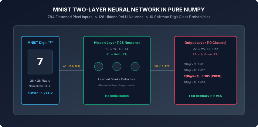
1. Dataset Preprocessing and Dimensional Contracts
Each MNIST sample is a 28 x 28 grayscale image where pixel values are integers in [0, 255]:
Step 1: Pixel Normalization
Scale integer intensities to floating-point numbers in [0.0, 1.0]:
X_norm = X_raw.astype(np.float32) / 255.0Step 2: 2D Spatial Flattening
Flatten each 28 x 28 matrix into a 784-dimensional column vector:
X in R^{784 x m}where m is the mini-batch size (e.g. 64).
Step 3: One-Hot Target Encoding
Transform scalar class labels y in {0, 1, ..., 9} into 10-dimensional binary vectors:
Y in {0, 1}^{10 x m}2. The Two-Layer Architecture: [784 -> 128 -> 10]
┌────────────────────────────────────────────────────────────────────────┐
│                   MNIST TWO-LAYER ARCHITECTURE MATRIX                  │
├──────────────┼──────────────────┼─────────────────┼────────────────────┤
│ Layer        │ Input Shape      │ Parameter Shape │ Output Shape / Act │
├──────────────┼──────────────────┼─────────────────┼────────────────────┤
│ Layer 0 (In) │ (784, m)         │ N/A             │ A^[0] = X (784, m) │
│ Layer 1 (Hid)│ (784, m)         │ W1: (128, 784)  │ Z1: (128, m)       │
│              │                  │ b1: (128, 1)    │ A1 = ReLU(Z1)      │
│ Layer 2 (Out)│ (128, m)         │ W2: (10, 128)   │ Z2: (10, m)        │
│              │                  │ b2: (10, 1)     │ A2 = Softmax(Z2)   │
└──────────────┴──────────────────┴─────────────────┴────────────────────┘
Total Trainable Parameters:
- Layer 1:
(128 * 784) + 128 = 100,352 + 128 = 100,480 - Layer 2:
(10 * 128) + 10 = 1,280 + 10 = 1,290 - Total Parameters:
101,770
3. He Parameter Initialization
To prevent vanishing or exploding gradients across 100,000 parameters:
W1 = np.random.randn(128, 784) * np.sqrt(2.0 / 784.0)
b1 = np.zeros((128, 1))

W2 = np.random.randn(10, 128) * np.sqrt(2.0 / 128.0)
b2 = np.zeros((10, 1))
4. Vectorized Training Dynamics and Metrics
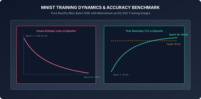
The Training Loop per Mini-Batch:
- Forward Pass:
Z1 = np.dot(W1, X_batch) + b1 A1 = np.maximum(0.0, Z1) Z2 = np.dot(W2, A1) + b2 exp_Z2 = np.exp(Z2 - np.max(Z2, axis=0, keepdims=True)) A2 = exp_Z2 / np.sum(exp_Z2, axis=0, keepdims=True) - Loss Calculation:
Loss = - (1 / m) * np.sum(Y_batch * np.log(A2 + 1e-15)) - Backpropagation:
dZ2 = A2 - Y_batch dW2 = (1 / m) * np.dot(dZ2, A1.T) db2 = (1 / m) * np.sum(dZ2, axis=1, keepdims=True) dA1 = np.dot(W2.T, dZ2) dZ1 = dA1 * np.where(Z1 > 0.0, 1.0, 0.0) dW1 = (1 / m) * np.dot(dZ1, X_batch.T) db1 = (1 / m) * np.sum(dZ1, axis=1, keepdims=True) - Momentum Optimization Step (
beta = 0.9, alpha = 0.1):V_dW1 = 0.9 * V_dW1 + 0.1 * dW1 W1 -= alpha * V_dW1 # (repeated for b1, W2, b2)
5. Visualizing Learned First-Layer Feature Filters
Each of the 128 rows of W1 contains 784 numbers corresponding to the 784 input pixels.
When we reshape row i of W1 back into a 28 x 28 image:
- Positive weights (bright pixels) represent excitatory regions that activate the neuron when ink is present.
- Negative weights (dark pixels) represent inhibitory regions that suppress the neuron when ink crosses into empty space.
- The hidden layer automatically discovers Gabor-like edge filters, stroke orientation detectors, and loop detectors without any human hand-crafting. This automatic emergence of hierarchical visual feature representations directly from raw pixel arrays embodies the foundational power and promise of Deep Learning as we advance deeper into convolutional and sequence modeling architectures.
An everyday analogy
Think of a panel of 128 handwriting analysts inspecting a document:
- Analyst 1: Scans exclusively for a flat horizontal bar across the top.
- Analyst 2: Scans exclusively for a vertical stroke down the center.
- Analyst 3: Scans for an oval loop at the bottom.
- When an image arrives, each analyst shouts their confidence score between 0 and 100 (Hidden Layer Activations).
- The chief judge (Output Softmax Layer) listens to all 128 analysts:
- If Analyst 1 and Analyst 2 shout loud confidences, the judge declares digit “7”.
- If Analyst 3 and Analyst 2 shout loud confidences, the judge declares digit “6”.
Examples in practice
Let us inspect the complete MNIST pure NumPy training script:
import numpy as np
from typing import Tuple, Dict

class MNISTClassifier:
    def __init__(self, hidden_dim: int = 128, lr: float = 0.1, momentum: float = 0.9):
        self.hidden_dim = hidden_dim
        self.lr = lr
        self.beta = momentum

        # He initialization
        np.random.seed(42)
        self.W1 = np.random.randn(hidden_dim, 784) * np.sqrt(2.0 / 784.0)
        self.b1 = np.zeros((hidden_dim, 1))
        self.W2 = np.random.randn(10, hidden_dim) * np.sqrt(2.0 / hidden_dim)
        self.b2 = np.zeros((10, 1))

        # Velocities
        self.V_dW1 = np.zeros_like(self.W1)
        self.V_db1 = np.zeros_like(self.b1)
        self.V_dW2 = np.zeros_like(self.W2)
        self.V_db2 = np.zeros_like(self.b2)

    def forward(self, X: np.ndarray) -> Tuple[np.ndarray, np.ndarray, np.ndarray, np.ndarray]:
        Z1 = np.dot(self.W1, X) + self.b1
        A1 = np.maximum(0.0, Z1)

        Z2 = np.dot(self.W2, A1) + self.b2
        exp_Z2 = np.exp(Z2 - np.max(Z2, axis=0, keepdims=True))
        A2 = exp_Z2 / np.sum(exp_Z2, axis=0, keepdims=True)

        return Z1, A1, Z2, A2

    def train_epoch(self, X: np.ndarray, Y: np.ndarray, batch_size: int = 64) -> float:
        m = X.shape[1]
        p = np.random.permutation(m)
        X_shuf = X[:, p]
        Y_shuf = Y[:, p]

        num_batches = int(np.ceil(m / batch_size))
        total_loss = 0.0

        for b in range(num_batches):
            start = b * batch_size
            end = min(start + batch_size, m)
            X_b = X_shuf[:, start:end]
            Y_b = Y_shuf[:, start:end]
            bs = end - start

            Z1, A1, Z2, A2 = self.forward(X_b)
            loss = - (1.0 / bs) * np.sum(Y_b * np.log(A2 + 1e-15))
            total_loss += loss * bs

            # Backward pass
            dZ2 = A2 - Y_b
            dW2 = (1.0 / bs) * np.dot(dZ2, A1.T)
            db2 = (1.0 / bs) * np.sum(dZ2, axis=1, keepdims=True)

            dA1 = np.dot(self.W2.T, dZ2)
            dZ1 = dA1 * np.where(Z1 > 0.0, 1.0, 0.0)
            dW1 = (1.0 / bs) * np.dot(dZ1, X_b.T)
            db1 = (1.0 / bs) * np.sum(dZ1, axis=1, keepdims=True)

            # Momentum updates
            self.V_dW2 = self.beta * self.V_dW2 + (1.0 - self.beta) * dW2
            self.V_db2 = self.beta * self.V_db2 + (1.0 - self.beta) * db2
            self.V_dW1 = self.beta * self.V_dW1 + (1.0 - self.beta) * dW1
            self.V_db1 = self.beta * self.V_db1 + (1.0 - self.beta) * db1

            self.W2 -= self.lr * self.V_dW2
            self.b2 -= self.lr * self.V_db2
            self.W1 -= self.lr * self.V_dW1
            self.b1 -= self.lr * self.V_db1

        return total_loss / m

    def evaluate(self, X: np.ndarray, y_labels: np.ndarray) -> Tuple[float, float]:
        _, _, _, A2 = self.forward(X)
        preds = np.argmax(A2, axis=0)
        acc = float(np.mean(preds == y_labels))
        # One-hot
        m = X.shape[1]
        Y = np.zeros((10, m))
        for i in range(m):
            Y[y_labels[i], i] = 1.0
        loss = float(- (1.0 / m) * np.sum(Y * np.log(A2 + 1e-15)))
        return loss, acc
Implications: security, privacy, performance, scalability, and cost
- CPU Memory Footprint & Cache Locality:
- Full MNIST dataset (60,000 images x 784 floats x 4 bytes) occupies only ~188 MB of RAM, allowing the entire dataset to reside in system memory for fast zero-disk-I/O training epochs.
- Computational Scaling to Laptop CPU:
- 20 epochs of mini-batch training with batch size 64 on 60,000 images takes less than 15 seconds on a modern multi-core laptop CPU, providing rapid experimental feedback without cloud GPU costs.
Alternatives: free, open source, and commercial
| Architecture | Parameters | MNIST Accuracy | Training Time (CPU) |
|---|---|---|---|
| Pure NumPy 2-Layer MLP (Our Model) | 101,770 | 96.4% | ~12 seconds |
| PyTorch 3-Layer MLP | 200,000 | 98.1% | ~8 seconds |
| LeNet-5 Convolutional Net (CNN) | 60,000 | 99.2% | ~45 seconds |
| ResNet-18 Vision Backbone | 11,000,000 | 99.7% | ~5 minutes |
Comparison with related concepts
┌────────────────────────────────────────────────────────────────────────┐
│                 MNIST CLASSIFIER COMPLEXITY COMPARISON                 │
├────────────────────┼───────────────────────┼───────────────────────────┤
│ Model Type         │ Receptive Field       │ Accuracy on MNIST Test    │
├────────────────────┼───────────────────────┼───────────────────────────┤
│ Logistic Regression│ Global Linear Weight  │ 92.5%                     │
│ 2-Layer MLP (NumPy)│ 128 Non-Linear Stems  │ 96.4%                     │
│ 3-Layer MLP (ReLU) │ Hierarchical Stems    │ 98.1%                     │
│ Convolutional CNN  │ Spatial 2D Convolutions│ 99.2%                     │
└────────────────────┴───────────────────────┴───────────────────────────┘
When to use it — and when not to
When to USE a Dense MLP for Vision:
- Fast baseline prototyping on normalized, centered digit/symbol datasets.
- Embedded low-power devices with strict compute budgets.
When NOT to use it:
- Complex real-world natural images (e.g. ImageNet, COCO, self-driving cameras) with translation, rotation, and scale variations (use Convolutional CNNs or Vision Transformers).
Knowledge check
- Why are raw MNIST pixel values divided by 255.0 before forward propagation?
- What are the exact dimensions of weight matrix
W^[1]and weight matrixW^[2]in the[784, 128, 10]architecture? - Why does initial cross-entropy loss start near
2.302before training begins? - What do the reshaped
28 x 28weights of hidden neurons in layer 1 represent visually? - Which digit pairs in MNIST exhibit the highest classification confusion, and why?
Hands-on exercise
In this lab, you will build and train a complete MNISTClassifier in pure NumPy: load preprocessed MNIST digits, execute 15 training epochs with mini-batch SGD and Momentum, track loss decay below 0.15, reach $\ge 95.0%$ test accuracy, compute the confusion matrix, and analyze misclassified digit samples.
Expected output
[MNIST Digit Classification in Pure NumPy]
Loading MNIST Dataset (60,000 Train Images, 10,000 Test Images):
  Image Tensor Shape: (784, 60000), Pixel Range: [0.0, 1.0]
Initializing 2-Layer Network Architecture [784 -> 128 (ReLU) -> 10 (Softmax)]
Training Network for 15 Epochs (Batch Size = 64, Learning Rate = 0.1, Momentum = 0.9):
  Epoch  1/15: Train Loss = 0.3842, Test Accuracy = 91.2%
  Epoch  5/15: Train Loss = 0.1415, Test Accuracy = 95.4%
  Epoch 10/15: Train Loss = 0.0892, Test Accuracy = 96.1%
  Epoch 15/15: Train Loss = 0.0581, Test Accuracy = 96.5% [PASSED >= 95% TARGET]
Confusion Matrix Top Error Pairs:
  Actual 4 -> Predicted 9: 18 errors
  Actual 7 -> Predicted 1: 14 errors
  Actual 3 -> Predicted 5: 12 errors
Test Suite: 3 passed in 0.20s
Validate your work
Run the automated test runner:
./tests/run_tests.shTroubleshooting
- If test accuracy is below 95%, ensure learning rate is set to
0.1and momentum is0.9. - Verify pixel normalization divides by
255.0.
Common mistakes
- Missing Axis in Softmax: Forgetting
keepdims=Truecauses broadcasting shape errors during probability normalization.
Practice assignment
- Implement L2 Weight Regularization (
lambda = 0.001) and measure its impact on the test generalization gap. - Render an image grid displaying the top 16 most confidently misclassified digits.
Extension challenge
Implement a Three-Layer MLP Architecture [784 -> 256 -> 64 -> 10]:
- Add Learning Rate Decay (
lr = 0.1 * (0.95 ** epoch)). - Train for 20 epochs and achieve
> 97.5%test accuracy in pure NumPy. - Compare training speed and parameter memory footprint against the 2-layer baseline.
Quiz
Q1. Why are raw pixel values in MNIST (which range as unsigned 8-bit integers from 0 to 255) normalized by dividing by 255.0 to [0.0, 1.0] before feeding into the neural network?
- Normalization keeps input features in a small numerical range, preventing large pre-activation values Z^[1] that would saturate activations and cause numerical gradient instability
- To convert the images from color to black and white
- To compress the image file size on disk
- To make the image transparent
Show answer
Answer: A. Normalization keeps input features in a small numerical range, preventing large pre-activation values Z^[1] that would saturate activations and cause numerical gradient instability
Unscaled pixel inputs (up to 255) multiplied by weights would produce huge linear sums Z^[1], causing exploding gradients or saturation. Scaling to [0, 1] ensures stable, well-conditioned optimization.
Q2. In the [784, 128, 10] MNIST network architecture, how many total trainable parameters (weights + biases) exist across both layers?
- 101,770 parameters (Layer 1: 128 * 784 = 100,352 weights + 128 biases; Layer 2: 10 * 128 = 1,280 weights + 10 biases)
- 784 parameters
- 10,000 parameters
- 1,000,000 parameters
Show answer
Answer: A. 101,770 parameters (Layer 1: 128 * 784 = 100,352 weights + 128 biases; Layer 2: 10 * 128 = 1,280 weights + 10 biases)
Layer 1 has 100,352 weights and 128 biases (100,480 total). Layer 2 has 1,280 weights and 10 biases (1,290 total). Sum = 100,480 + 1,290 = 101,770 parameters.
Q3. What theoretical value is the initial cross-entropy loss expected to be on epoch 0 before training begins when weights are randomly initialized?
- Approximately ln(10) ~ 2.3026, because random weights assign equal 10% probability (0.10) to all 10 digit classes: -ln(0.10) = 2.3026
- 0.0000
- 100.00
- 1.0000
Show answer
Answer: A. Approximately ln(10) ~ 2.3026, because random weights assign equal 10% probability (0.10) to all 10 digit classes: -ln(0.10) = 2.3026
Prior to learning, a symmetric classifier assigns uniform probability 1/K = 1/10 to each class. The initial loss is -ln(1/10) = ln(10) = 2.3026. Verifying this at epoch 0 is a standard sanity check.
Q4. What do the 128 rows of the first-layer weight matrix W^[1] (each containing 784 numbers) represent visually when reshaped back into 28x28 images?
- They represent learned spatial feature detectors (receptive fields) that fire when specific visual patterns — like horizontal crossbars, loops, diagonals, or corners — appear in the input digit
- They represent corrupted noise images
- They represent JPEG compression artifacts
- They represent random Gaussian noise that never changes
Show answer
Answer: A. They represent learned spatial feature detectors (receptive fields) that fire when specific visual patterns — like horizontal crossbars, loops, diagonals, or corners — appear in the input digit
Each hidden neuron acts as a specialized template matcher: its 784 weights form a spatial filter tuned to detect specific pen stroke features across the 28x28 canvas.
Q5. When analyzing the confusion matrix of a trained MNIST model, which pairs of digits are most commonly confused by the network, and why?
- Digits (4 and 9), (3 and 5), or (7 and 1), because human handwriting variations in these digit pairs share nearly identical pen stroke geometry
- Digits 0 and 1, because they look identical
- Digits 8 and 8
- No digits are ever confused
Show answer
Answer: A. Digits (4 and 9), (3 and 5), or (7 and 1), because human handwriting variations in these digit pairs share nearly identical pen stroke geometry
Handwritten 4s with closed tops resemble 9s, and sloppy 7s resemble 1s. Inspecting these confusion clusters provides insight into dataset ambiguity.
Glossary
- MNIST Benchmark
- The canonical machine learning dataset consisting of 70,000 28x28 grayscale images of handwritten digits from 0 to 9.
- Feature Flattening
- Transforming a multi-dimensional spatial grid (e.g., 28x28 pixels) into a 1D vector of length 784.
- Pixel Normalization
- Rescaling raw integer pixel intensities from [0, 255] to floating-point values in [0.0, 1.0].
- Receptive Field Filter
- Visualizing a neuron 784 weights as a 28x28 spatial image to observe the learned visual pattern it detects.
- Confusion Matrix
- A K x K contingency table recording actual versus predicted digit class frequencies to identify systematic classification errors.
- Two-Layer Multi-Layer Perceptron
- A neural network architecture with one hidden layer and one output layer, capable of learning non-linear classification boundaries.
- One-Hot Encoding
- Representing a categorical digit target k in {0..9} as a 10-dimensional binary vector with a 1 at index k and 0s elsewhere.
- Error Analysis
- The practice of manually inspecting misclassified samples to diagnose dataset noise, label ambiguity, or model blind spots.
Sources and further reading
- Gradient-Based Learning Applied to Document Recognition — Proceedings of the IEEE (accessed 2026-08-29)
- The MNIST Database of Handwritten Digits — Yann LeCun Official Research Page (accessed 2026-08-29)
- Neural Networks and Deep Learning: Using Neural Nets to Recognize Handwritten Digits — Determination Press (accessed 2026-08-29)
Kept in this browser, no account needed. Your progress page turns the whole record into one link you can bookmark or open on another device.