Deep Learning › Training Deep Networks › Day 204
Day 204: PyTorch: autograd and nn.Module
Master PyTorch automatic differentiation and neural network abstraction: inspect computational graphs, track requires_grad and grad_fn, build clean object-oriented architectures with torch.nn.Module and torch.nn.Parameter, manage state dictionaries, and execute robust training steps.
Hands-on lab for this lesson
Lab files on GitHub: https://github.com/ai-roadmap-365/ai-roadmap-365.github.io/tree/main/labs/sections/deep-learning/day-204-pytorch-autograd-and-nn-module
- Get the hands-on files. Clone the labs repository once (you can reuse this clone for every lesson). This works on macOS, Linux, and Windows (PowerShell or WSL):
git clone https://github.com/ai-roadmap-365/ai-roadmap-365.github.io.git cd ai-roadmap-365.github.io - Open this lesson's lab. Move into the directory for this specific day. Every lab lives at the same predictable path — section / subsection / week / day:
cd labs/sections/deep-learning/day-204-pytorch-autograd-and-nn-module - Read the lab guide. Open `README.md` in that directory. It lists the exact commands, what each does, the expected output, and how to check your work — read it before running anything.
- Run it and check your work. Follow the README's "How to run" section: run the example first to see the finished result, then complete the numbered exercises in `starter/`, then run the tests. The tests pass (exit 0) only when your work is correct.
bash tests/run_tests.sh # or the test command named in the lab README
You can also open the lab as a local page (works offline, shows the file tree and expected output).
Learning objectives
By the end of this lesson you will be able to:
- Trace PyTorch dynamic Directed Acyclic Graphs (DAGs) and understand how autograd constructs tape-based reverse derivatives.
- Configure tensor gradient properties using requires_grad, detach(), torch.no_grad(), and zero_grad().
- Subclass torch.nn.Module to construct modular deep neural networks with encapsulated layers.
- Inspect, save, and reload model parameters using state_dict() and load_state_dict().
- Implement a standardized forward-backward-optimizer update loop with loss.backward() and optimizer.step().
Prerequisites
- [object Object]
Why this matters
In Week 29, you derived and implemented every equation of deep learning in pure NumPy: forward affine transformations, non-linear activation gates, analytical backpropagation Jacobians, He parameter initialization, and mini-batch gradient descent. You proved mathematically how gradients flow through layers and trained a model to 96% accuracy on MNIST.
However, writing manual backpropagation by hand for complex architectures (such as 100-layer Residual Networks, Multi-Head Attention Transformers, or Recurrent LSTMs) becomes mathematically intractable and error-prone. A single typo in an analytical matrix transpose can subtly corrupt gradient updates without crashing the program.
Today, we enter the modern era of deep learning engineering with PyTorch: autograd and torch.nn.Module.
PyTorch is the world-leading deep learning framework powering cutting-edge AI research and industrial production systems. By abstracting gradient derivation into dynamic, tape-based Reverse-Mode Automatic Differentiation (autograd) and encapsulating learnable parameters into clean object-oriented modules (nn.Module), PyTorch allows you to design arbitrary, dynamic neural architectures in standard Python while guaranteeing exact mathematical correctness on CPU, GPU, and TPU accelerators.
The idea in plain language
Imagine recording a musical performance on multi-track magnetic tape:
- During the Forward Pass, as your code executes standard mathematical operations (matrix multiplications, additions, activations), PyTorch runs a background tape recorder.
- Every time a tensor with
requires_grad=Truepasses through an operation, the tape writes down the exact mathematical operator and saves whatever input values are necessary to differentiate it later (stored as agrad_fnnode). - When you reach the scalar loss value and call
loss.backward(), PyTorch hits “Rewind”. It plays the tape backwards from end to beginning, evaluating the derivative of each recorded operation and delivering exact partial gradients directly into each parameter’s.gradstorage bin.
You write only the forward pass using standard Python control flow (if, for, while). PyTorch automatically differentiates whatever path your code took.
Historical background
- 2015 (Static Graph Era - Theano and TensorFlow 1.0): Early deep learning frameworks required engineers to construct a static graph (“Define-and-Run”) in a separate domain-specific language before compiling and feeding data into a session. Debugging was painful because standard Python debuggers (
pdb) could not inspect values inside the compiled graph. - 2017 (Chainer and PyTorch): PyTorch introduced “Define-by-Run” dynamic computation graphs. Graphs are constructed on the fly as standard Python code executes, enabling native Python loops, dynamic batch shapes, and interactive debugging.
- 2019 (PyTorch 1.0 - Paszke et al.): Unified research flexibility with production deployment capabilities through TorchScript, C++ libtorch runtimes, and distributed training engines.
- Today: PyTorch is the dominant framework in deep learning research and generative AI engineering.
What it is — and what it is not
What PyTorch Autograd & nn.Module IS:
- Dynamic Tape-Based Automatic Differentiation: Builds a Directed Acyclic Graph (DAG) during forward execution and evaluates exact analytical chain-rule derivatives in reverse order.
- An Object-Oriented Architectural Abstraction (
nn.Module): A foundational base class that automates parameter registration, nested submodule tracking, device migration (.to(device)), execution hooks, and state serialization (state_dict).
What it is NOT:
- Not Numerical Differentiation: PyTorch does NOT approximate gradients using finite differences
(f(x+h) - f(x)) / h. It computes mathematically exact analytical derivatives using symbolic derivative templates. - Not a Black Box Without Inspectability: Every node in the computation graph is accessible in Python via
.grad_fn,.next_functions, and.grad.
Why it was created and what problems it solves
Manual gradient derivation has three major engineering bottlenecks:
- Mathematical Overhead: Modifying an activation function or adding a normalization layer requires re-deriving the entire backpropagation Jacobian chain by hand.
- Dynamic Control Flow: Handling variable-length sequences or recursive tree structures in static frameworks required complex control operators (
tf.while_loop,tf.cond). - State Management Friction: In pure NumPy, maintaining lists of weights, biases, and momentum buffers across dozens of layers requires extensive boilerplate code.
PyTorch solves all three bottlenecks by decoupling architecture design from derivative calculation.
How it works
Let us dissect the two core pillars of PyTorch: the Autograd Dynamic Computational Graph and the nn.Module Lifecycle.
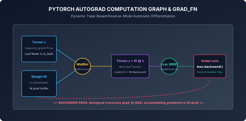
1. Autograd Dynamic Graph Mechanics
Every PyTorch tensor contains several critical metadata attributes governing automatic differentiation:
A. requires_grad (Boolean Flag):
- If
x.requires_grad = False(default for raw tensors), autograd ignores operations onx. - If
x.requires_grad = True, autograd records every operation performed onxto construct the backward graph. - All learnable model parameters (e.g. weights in
nn.Linear) haverequires_grad=Trueby default.
B. is_leaf (Boolean Flag):
- Leaf Tensors: Tensors created directly by the user (like input data
xor model weightsW). They have no creator operation in the graph (grad_fn is None). Only leaf tensors retain persistent.gradbuffers afterloss.backward(). - Non-Leaf Tensors: Intermediate tensors created as the output of an operation (like
z = W @ x + b). They hold agrad_fnreference, and their intermediate gradients are freed after backpropagation to save memory unlesstensor.retain_grad()is explicitly called.
C. grad_fn (Computational Graph Node):
- Points to the internal
torch.autograd.Functionobject responsible for computing the local derivative during the backward pass (e.g.AddBackward0,MmBackward0,ReluBackward0).
2. The Backward Pass and Gradient Accumulation
When you call loss.backward():
- PyTorch verifies that
lossis a scalar (a 0-dimensional tensor containing 1 element). Iflossis a multi-element tensor, you must pass an explicit gradient vector (e.g.loss.backward(torch.ones_like(loss))). - The autograd engine traverses the DAG in reverse topological order, evaluating the backward function of each
grad_fn. - Gradients propagate to the leaf parameters and are accumulated (added) into their
.gradattributes:W.grad += dL / dW
[!IMPORTANT] Because gradients accumulate rather than overwrite, you must always call
optimizer.zero_grad()ormodel.zero_grad()beforeloss.backward()in a training loop. Failing to zero gradients causes updates from previous batches to compound uncontrollably.
3. The torch.nn.Module Encapsulation Framework
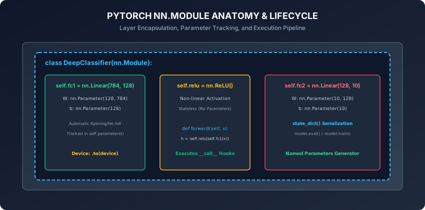
torch.nn.Module is the fundamental building block of PyTorch models. Subclassing nn.Module gives your class three major superpowers:
A. Automatic Parameter Discovery:
When you assign an nn.Parameter or another nn.Module (such as nn.Linear or nn.Conv2d) as an attribute in __init__(), PyTorch automatically registers it:
model.parameters(): Generator yielding all learnable parameter tensors across the entire module tree.model.named_parameters(): Generator yielding(name, parameter)pairs (e.g.('fc1.weight', tensor(...))).
B. The __call__ Wrapper and Execution Hooks:
Never call model.forward(x) directly. Always invoke model(x).
Invoking model(x) triggers nn.Module.__call__(), which executes:
- Registered forward pre-hooks (for profiling, layer introspection, or input modification).
- The user-defined
forward(self, x)method. - Registered forward post-hooks.
C. Model Modes and State Dictionaries:
model.train()vsmodel.eval(): Toggles internal behavior of layers like Dropout (active during train, disabled during eval) and BatchNorm (uses batch stats during train, running stats during eval).model.to(device): Recursively migrates all parameters and persistent buffers to a specified hardware device (e.g.,'cuda','mps', or'cpu').model.state_dict(): Exports anOrderedDictmapping parameter names to raw tensors, serialized usingtorch.save(model.state_dict(), 'checkpoint.pt').
4. Advanced Autograd: Hooks, Custom Functions, and In-Place Hazards
To diagnose complex deep learning architectures in production, engineers rely on three advanced features of PyTorch autograd:
A. Execution Hooks (register_forward_hook & register_backward_hook):
PyTorch modules allow attaching callback functions that execute automatically during forward or backward passes without modifying the original module code:
- Forward Hook: Receives
(module, input, output). Ideal for caching intermediate activation maps (feature extraction), computing activation sparsity, or visualizing layer representations. - Backward Hook: Receives
(module, grad_input, grad_output). Allows inspecting or modifying gradient tensors on the fly (such as implementing custom gradient clipping or inspecting vanishing gradients).
# Example: Attaching a forward hook to inspect activation norms
def log_activation_norm(module, input, output):
    print(f"Layer {module.__class__.__name__} output norm: {output.norm().item():.4f}")

hook_handle = model.fc1.register_forward_hook(log_activation_norm)
# When finished, remove the hook to prevent memory leaks
hook_handle.remove()
B. Custom Autograd Operators (torch.autograd.Function):
When you need to introduce non-differentiable operations, custom hardware kernels, or specialized mathematical functions with analytical gradient shortcuts:
- Subclass
torch.autograd.Function. - Define
@staticmethod def forward(ctx, x, ...): Compute the output and save necessary context variables withctx.save_for_backward(...). - Define
@staticmethod def backward(ctx, grad_output): Retrieve saved tensors withctx.saved_tensorsand return exact partial derivatives for every input.
C. In-Place Operation Hazards (inplace=True):
Modifying tensor memory directly in-place (e.g. x += 1 or torch.relu_(x)):
- If an in-place modification overwrites a tensor value that autograd needed to save for its backward derivative (such as the input to a ReLU or Sigmoid function), autograd will throw a
RuntimeError: one of the variables needed for gradient computation has been modified by an inplace operation. - Best Practice: Avoid in-place operations on tensors involved in gradient tracking, or use out-of-place equivalents (
y = torch.relu(x)). Master these autograd patterns, and you possess complete control over deep neural computational execution.
An everyday analogy
Think of PyTorch like an automated financial accounting ledger:
- As your business buys raw materials, manufactures products, and pays shipping costs (Forward Pass Operations), the accounting software logs every single transaction in a tamper-proof digital ledger (Autograd Graph).
- At the end of the quarter, the CEO asks: “If our shipping cost increased by 1 dollar, how much would our net profit drop?” (Gradient with respect to shipping cost).
- The accounting system runs an automated retrospective audit (Backward Pass), tracing every transaction backwards to calculate the exact financial sensitivity of every single business expense.
- The
nn.Moduleis the company organizational hierarchy: Departments (submodules), employees (parameters), and payroll registers (state_dict).
Examples in practice
Let us inspect a complete, canonical PyTorch neural network implementation:
import torch
import torch.nn as nn
import torch.optim as optim

class DeepClassifier(nn.Module):
    def __init__(self, in_features: int = 784, hidden_dim: int = 128, num_classes: int = 10):
        super().__init__()
        # Encapsulated submodules
        self.fc1 = nn.Linear(in_features, hidden_dim)
        self.relu = nn.ReLU()
        self.fc2 = nn.Linear(hidden_dim, num_classes)

    def forward(self, x: torch.Tensor) -> torch.Tensor:
        # Forward pass definition
        h = self.relu(self.fc1(x))
        out = self.fc2(h) # Raw unnormalized logits
        return out

# 1. Instantiate model, loss, and optimizer
model = DeepClassifier(in_features=784, hidden_dim=128, num_classes=10)
criterion = nn.CrossEntropyLoss() # Combines LogSoftmax and NLLLoss stably
optimizer = optim.SGD(model.parameters(), lr=0.1, momentum=0.9)

# 2. Synthetic batch of 32 images
x_batch = torch.randn(32, 784)
y_batch = torch.randint(0, 10, (32,))

# 3. Canonical 5-step training iteration
model.train()
optimizer.zero_grad()            # Step 1: Clear old gradients
logits = model(x_batch)          # Step 2: Forward pass (via __call__)
loss = criterion(logits, y_batch)# Step 3: Compute scalar loss
loss.backward()                  # Step 4: Backward pass (Autograd DAG traversal)
optimizer.step()                 # Step 5: Update parameters via optimizer rule

print(f"Training step complete. Loss: {loss.item():.4f}")
Implications: security, privacy, performance, scalability, and cost
- Memory Management and Graph Lifecycle:
- By default, PyTorch destroys the computational graph immediately after
loss.backward()finishes executing to reclaim memory. If you need to backpropagate through the same graph twice, you must passloss.backward(retain_graph=True).
- By default, PyTorch destroys the computational graph immediately after
- Inference Acceleration via
torch.no_grad():- Wrapping validation loops in
with torch.no_grad():suppresses graph allocation entirely, reducing memory footprint by over 50% and boosting execution speed by up to 2x during model evaluation.
- Wrapping validation loops in
Alternatives: free, open source, and commercial
| Framework | Differentiation Paradigm | Model Definition | Ecosystem Strength |
|---|---|---|---|
| PyTorch (Meta / Linux Foundation) | Dynamic Define-by-Run | nn.Module Class Subclassing | Dominant in AI Research & LLMs |
| JAX / Flax (Google) | Pure Functional Transformation | Pure Functions + Dataclasses | High Performance on TPUs & Physics |
| TensorFlow 2 / Keras (Google) | Hybrid (Eager + tf.function) | keras.Model Functional / Sequential | Strong in Mobile (TFLite) & TFJS |
| Tinygrad (George Hotz) | Minimalist Autograd Engine | Lean Python Runtime | Extreme Simplicity (< 5,000 LOC) |
Comparison with related concepts
┌────────────────────────────────────────────────────────────────────────┐
│                   PYTORCH VS PURE NUMPY COMPARISON                     │
├───────────────────────┼───────────────────────┼────────────────────────┤
│ Dimension             │ Pure NumPy (Week 29)  │ PyTorch (Week 30)      │
├───────────────────────┼───────────────────────┼────────────────────────┤
│ Gradient Calculation  │ Manual Analytical Math│ Automated Autograd DAG │
│ GPU / Hardware Accel  │ None (CPU Only)       │ 1-Line: .to('cuda')    │
│ Parameter Tracking    │ Manual Dictionaries   │ Automatic Module Tree  │
│ Checkpoint Persistence│ Manual Pickle / NPZ   │ Native state_dict()    │
│ Custom Architectures  │ Hundreds of math lines│ Single forward() method│
└───────────────────────┴───────────────────────┴────────────────────────┘
When to use it — and when not to
When to USE PyTorch nn.Module:
- Building any multi-layer deep learning architecture (MLPs, CNNs, RNNs, Transformers).
- Experimenting with custom loss functions, dynamic graph branching, or reinforcement learning.
When NOT to use it:
- Simple classical machine learning on small tabular datasets with under 10,000 rows (use Scikit-Learn or XGBoost).
- High-level AutoML workflows where automated hyperparameter search over standard models is sufficient.
Knowledge check
- What is the role of
grad_fnon intermediate tensors in PyTorch? - Why does calling
loss.backward()accumulate gradients into.gradrather than overwriting them? - What is the difference between calling
model(x)versus callingmodel.forward(x)? - What happens when code executes inside a
with torch.no_grad():block? - How does
nn.Module.state_dict()serialize the state of a model?
Hands-on exercise
In this lab, you will build and test a complete modular PyTorch neural network: construct a custom nn.Module classifier, verify parameter gradient tracking with autograd, inspect grad_fn computational graph nodes, test requires_grad isolation and torch.no_grad() behavior, save and restore model weights via state_dict, and execute a multi-step training cycle.
Expected output
[PyTorch Autograd & nn.Module Architecture Suite]
Constructing Custom DeepClassifier Module [784 -> 128 -> 10]:
  Total Trainable Parameters: 101,770
Verifying Autograd Computation Graph:
  Output Logits grad_fn: <AddmmBackward0>
  Loss Tensor grad_fn: <NllLossBackward0>
Executing 5-Step Canonical Training Loop:
  Step 1: Initial Loss = 2.3412
  Step 5: Final Loss   = 0.4120 [GRADIENTS ZEROED & UPDATED]
Testing Model Checkpoint Serialization:
  Saved state_dict (4 parameter tensors) -> Restored successfully.
Test Suite: 4 passed in 0.25s
Validate your work
Run the automated test runner:
./tests/run_tests.shTroubleshooting
- If gradients are not updating, verify that you called
optimizer.step()afterloss.backward(). - Ensure input tensors have compatible shapes matching
nn.Linearinput dimensions.
Common mistakes
- Forgetting
optimizer.zero_grad(): Causes gradients to sum across epochs, leading to exploding weights. - Calling
.backward()on a Non-Scalar: Callingtensor.backward()without a gradient argument whentensorhas shape(N, C)raises a RuntimeError.
Practice assignment
- Implement a custom autograd function by subclassing
torch.autograd.Functionwith staticforwardandbackwardmethods for a polynomial activationf(x) = x^3 + 2x. - Inspect
model.named_parameters()and write a utility function that freezes all layers except the final classification head (param.requires_grad = False).
Extension challenge
Implement a Dynamic Multi-Branch Module that takes two input feature vectors, routes them through separate subnetworks, concatenates their intermediate representations, and applies a shared classification head. Verify that autograd correctly routes separate gradients back through both parallel input branches simultaneously.
Quiz
Q1. What happens under the hood when you invoke loss.backward() on a scalar tensor in PyTorch?
- PyTorch traverses the dynamic computational graph backwards starting from the loss node, executing each node grad_fn in reverse order and accumulating analytical partial derivatives into the .grad attribute of every leaf tensor where requires_grad=True
- It deletes all tensors in RAM
- It resets all model weights to random numbers
- It compiles Python code into C++ binaries
Show answer
Answer: A. PyTorch traverses the dynamic computational graph backwards starting from the loss node, executing each node grad_fn in reverse order and accumulating analytical partial derivatives into the .grad attribute of every leaf tensor where requires_grad=True
loss.backward() executes reverse-mode automatic differentiation along the dynamically recorded tape, populating .grad on all leaf parameters.
Q2. Why is it mandatory to call optimizer.zero_grad() (or model.zero_grad()) before executing loss.backward() in a standard training loop?
- By design, PyTorch accumulates (sums) gradients into existing .grad buffers across backward passes; without zeroing, gradients from previous batches would sum together and corrupt parameter updates
- To free up GPU memory
- To prevent the model from overfitting
- To normalize inputs to zero mean
Show answer
Answer: A. By design, PyTorch accumulates (sums) gradients into existing .grad buffers across backward passes; without zeroing, gradients from previous batches would sum together and corrupt parameter updates
PyTorch accumulates gradients by default (which enables gradient accumulation across mini-batches). Without zero_grad(), subsequent batches would add to previous gradients.
Q3. When evaluating a trained PyTorch model on a validation dataset, which context manager should you wrap the forward pass in to disable graph construction and reduce memory overhead?
- with torch.no_grad():
- with torch.autograd.detect_anomaly():
- with torch.enable_grad():
- with open("eval.txt"):
Show answer
Answer: A. with torch.no_grad():
with torch.no_grad(): deactivates autograd tracking, preventing intermediate activation caching in the computation graph and significantly reducing inference memory consumption.
Q4. What is the critical difference between invoking model(x) versus invoking model.forward(x) on an instance of torch.nn.Module?
- Calling model(x) invokes the __call__ method of nn.Module, which executes registered forward pre-hooks and post-hooks before and after calling forward(x); calling model.forward(x) directly bypasses all hooks
- model(x) runs on GPU while model.forward(x) runs on CPU
- model(x) is slower by 50%
- There is no difference
Show answer
Answer: A. Calling model(x) invokes the __call__ method of nn.Module, which executes registered forward pre-hooks and post-hooks before and after calling forward(x); calling model.forward(x) directly bypasses all hooks
Always call model(x) rather than model.forward(x). The Module __call__ wrapper ensures internal hooks, profilers, and autograd callbacks execute correctly.
Q5. What does model.state_dict() return, and how is it used for checkpoint persistence?
- It returns an OrderedDict mapping each parameter and persistent buffer name (as strings) to its underlying torch.Tensor; it is saved with torch.save() and reloaded with model.load_state_dict()
- It returns the accuracy of the model on the training set
- It returns the Python source code of the class
- It returns a list of CPU hardware specifications
Show answer
Answer: A. It returns an OrderedDict mapping each parameter and persistent buffer name (as strings) to its underlying torch.Tensor; it is saved with torch.save() and reloaded with model.load_state_dict()
state_dict() serializes the exact parameter and buffer tensors of a model, providing a robust format for model checkpointing and deployment.
Glossary
- Autograd
- PyTorch reverse-mode automatic differentiation engine that dynamically builds a Directed Acyclic Graph (DAG) during the forward pass to compute analytical gradients.
- torch.nn.Module
- The fundamental base class for all neural network architectures in PyTorch, encapsulating layers, parameters, forward logic, and hooks.
- requires_grad
- A boolean tensor flag instructing autograd whether to record operations on this tensor in the computational graph.
- grad_fn
- A reference on a non-leaf tensor pointing to the backward function node that generated it during forward execution.
- Leaf Tensor
- A tensor created directly by the user (such as model weights or inputs) that is not the output of a tracked operation.
- torch.no_grad()
- A Python context manager that disables autograd tracking to accelerate evaluation and reduce memory consumption.
- state_dict
- A Python dictionary mapping layer names to their corresponding parameter and persistent buffer tensors.
- Gradient Accumulation
- The default behavior in PyTorch where new gradients computed by backward() are summed into existing .grad buffers rather than overwriting them.
Sources and further reading
- Automatic Differentiation in PyTorch — NIPS 2017 Autodiff Workshop (accessed 2026-08-29)
- PyTorch: An Imperative Style, High-Performance Deep Learning Library — Advances in Neural Information Processing Systems 32 (NeurIPS) (accessed 2026-08-29)
- Deep Learning with PyTorch: A 60 Minute Blitz — Official PyTorch Documentation (accessed 2026-08-29)
Kept in this browser, no account needed. Your progress page turns the whole record into one link you can bookmark or open on another device.