Deep Learning › Sequences and Text › Day 220
Day 220: Recurrent Neural Networks
Master stateful sequential computation: derive recurrent hidden state transition equations, unroll computational graphs across time, implement Backpropagation Through Time (BPTT) from scratch, analyze vanishing and exploding gradient mechanics, apply gradient norm clipping, and build a character-level sequence generator in PyTorch.
Hands-on lab for this lesson
Lab files on GitHub: https://github.com/ai-roadmap-365/ai-roadmap-365.github.io/tree/main/labs/sections/deep-learning/day-220-recurrent-neural-networks
- Get the hands-on files. Clone the labs repository once (you can reuse this clone for every lesson). This works on macOS, Linux, and Windows (PowerShell or WSL):
git clone https://github.com/ai-roadmap-365/ai-roadmap-365.github.io.git cd ai-roadmap-365.github.io - Open this lesson's lab. Move into the directory for this specific day. Every lab lives at the same predictable path — section / subsection / week / day:
cd labs/sections/deep-learning/day-220-recurrent-neural-networks - Read the lab guide. Open `README.md` in that directory. It lists the exact commands, what each does, the expected output, and how to check your work — read it before running anything.
- Run it and check your work. Follow the README's "How to run" section: run the example first to see the finished result, then complete the numbered exercises in `starter/`, then run the tests. The tests pass (exit 0) only when your work is correct.
bash tests/run_tests.sh # or the test command named in the lab README
You can also open the lab as a local page (works offline, shows the file tree and expected output).
Learning objectives
By the end of this lesson you will be able to:
- Derive the hidden state recurrence equation h_t = tanh(W_hh * h_prev + W_xh * x_t + b_h) from first principles.
- Unroll recurrent computational graphs across time and implement Backpropagation Through Time (BPTT).
- Mathematically analyze the Jacobian product leading to exponential vanishing and exploding gradients.
- Implement gradient norm clipping to stabilize recurrent training loops.
- Construct, train, and sample from a character-level language generation RNN in pure PyTorch.
Prerequisites
Why this matters
Feedforward neural networks (like MLPs and CNNs) operate under a rigid architectural constraint: they assume all input samples are independent and identically distributed (i.i.d.).
However, the vast majority of real-world information is fundamentally sequential and temporal:
- Natural language sentences (where the meaning of word #10 depends on word #1).
- Time series financial stock prices and sensor telemetry.
- Audio speech signals, music waveforms, and biological DNA strings.
If you pass a sentence into a feedforward network as a flat vector, the network cannot easily handle variable-length inputs and is blind to word order.
In 1990, cognitive scientist Jeffrey Elman introduced the Simple Recurrent Neural Network (Elman RNN). By adding a recurrent feedback loop that passes an internal Hidden State Vector ($h_t$) from one time step to the next, neural networks gained an internal memory buffer.
Today, you will master the mechanics of recurrent networks: unrolling computation graphs across time, deriving Backpropagation Through Time (BPTT), diagnosing the mathematical causes of vanishing and exploding gradients, implementing gradient norm clipping, and building a character-level sequence generator in PyTorch.
The idea in plain language
Imagine reading a thrilling murder mystery novel:
- Feedforward Network (Amnesia Reader): You read each word in complete isolation. When you read page 200 and see the word
"guilty", you have already forgotten every clue, character, and plot twist from pages 1 through 199. - Recurrent Neural Network (Reader with a Mental Notepad): As you read each word $x_t$, you maintain a mental summary of the story on your notepad (Hidden State $h_t$).
- When you read a new word $x_t$, you combine the new word with your current summary $h_(t-1)$ to write an updated summary $h_t$.
- When you finish the chapter, your final notepad state $h_T$ contains the distilled context of the entire story.
Historical background

- 1986 (Rumelhart, Hinton, & Williams): Introduced Backpropagation Through Time (BPTT), showing that unrolling recurrent networks into deep feedforward graphs allowed standard gradient descent to train temporal states.
- 1990 (Jeffrey Elman & Elman RNNs): Introduced the simple recurrent network architecture ($h_t = \sigma(W_(hh) h_(t-1) + W_(xh) x_t)$), demonstrating that networks could learn grammar and syntactic word boundaries without explicit rules.
- 1994 (Bengio et al. & The Vanishing Gradient Proof): Yoshua Bengio et al. published the mathematical proof explaining why gradient descent struggled on long temporal sequences: repeated Jacobian matrix multiplications caused gradients to vanish exponentially.
- 2013 (Mikolov, Pascanu, & Gradient Clipping): Razvan Pascanu, Tomas Mikolov, and Yoshua Bengio systematized gradient clipping to eliminate exploding gradients, enabling large-scale RNN training.
What it is — and what it is not
What an RNN IS:
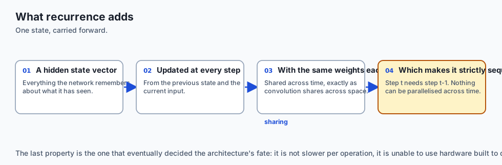
- A State-Space Dynamical System: A network that updates a persistent continuous state vector $h_t$ at every discrete time step $t$ using the transition function $h_t = f(h_(t-1), x_t)$.
- Time-Invariant Parameter Sharing: The exact same weight matrices ($W_(xh), W_(hh), W_(hy)$) are reused across every time step $t \in [1, T]$.
What it is NOT:
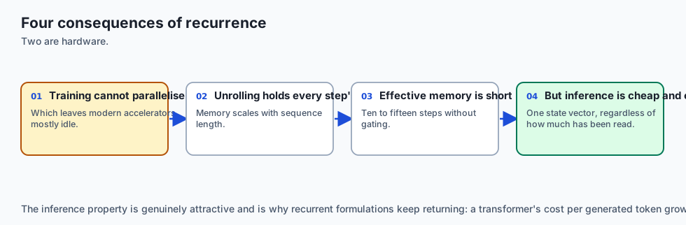
- Not Infinite Memory: Standard vanilla RNNs suffer from catastrophic forgetting: after 10 to 15 time steps, early inputs vanish from the hidden state. (Longer temporal retention requires LSTMs and GRUs, which we study tomorrow in Day 221).
- Not Parallelizable Across Time: Because $h_t$ strictly requires $h_(t-1)$, training cannot compute step $t$ until step $t-1$ completes, creating a sequential compute bottleneck on GPUs.
Why it was created and what problems it solves
Recurrent networks resolved three critical limitations of classical feedforward architectures:
- Handling Arbitrary Variable Sequence Lengths: Feedforward networks require fixed input dimensions ($N$ inputs). An RNN processes sequences of length 3, 30, or 300 using the identical weight tensors.
- Temporal Equivariance: A phrase like
"not good"produces a similar shift in hidden state whether it appears at word #2 or word #50. - Flexible Sequence Topologies:
- Many-to-One: Sentiment analysis (Sequence of words $\rightarrow$ Single sentiment class).
- One-to-Many: Image captioning (Single image vector $\rightarrow$ Sequence of generated words).
- Many-to-Many (Synchronized): Video frame classification or Part-of-Speech tagging.
- Many-to-Many (Delayed / Seq2Seq): Machine translation (Full input sentence $\rightarrow$ Full output translation).
How it works
Let us dissect the mathematical formulation of recurrent forward propagation and Backpropagation Through Time.
1. Forward Propagation Equations
At each discrete time step $t \in [1, T]$:
-
Receive input vector $x_t \in R^(d_(\text(in)))$ (e.g. word embedding) and previous hidden state $h_(t-1) \in R^(d_h)$.
-
Compute the new hidden state using the non-linear hyperbolic tangent activation ($\tanh$):
h_t = tanh(W_{xh} * x_t + W_{hh} * h_{t-1} + b_h) -
Compute the output prediction logits $\hat(y)t \in R^(d(\text(out)))$:
\hat{y}_t = W_{hy} * h_t + b_y -
For multi-class classification / language modeling, compute the softmax probability distribution:
p_t = softmax(\hat{y}_t)
2. Backpropagation Through Time (BPTT)
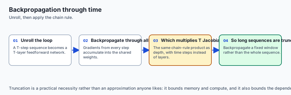
To train the shared parameters ($W_(xh), W_(hh), W_(hy)$), we compute total sequence loss $L = \sum_(t=1)^T L_t$.
By the multivariate chain rule, the gradient of loss at step $T$ with respect to the recurrent weight matrix $W_(hh)$ accumulates across all prior time steps:
partial L_T / partial W_{hh} = sum_{k=1}^T (partial L_T / partial h_T) * (partial h_T / partial h_k) * (partial h_k / partial W_{hh})The crucial term is the temporal Jacobian product:
partial h_T / partial h_k = prod_{j=k+1}^T (partial h_j / partial h_{j-1}) = prod_{j=k+1}^T W_{hh}^\top * diag(1 - h_j^2)3. The Mathematics of Vanishing and Exploding Gradients
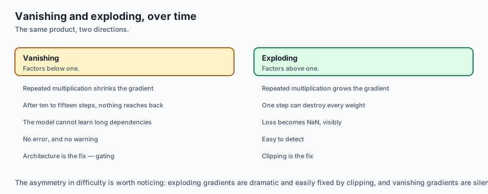
The Jacobian product involves multiplying $T - k$ matrices together:
-
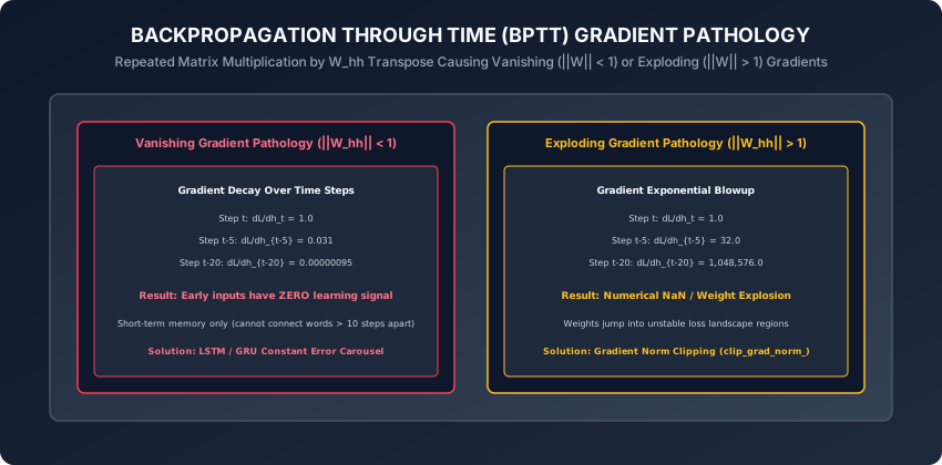
Case 1: Vanishing Gradients ($|W_(hh)|_2 < 1$): Since $\tanh’(z) = 1 - \tanh^2(z) \le 1$, if the largest singular value of $W_(hh)$ is $\lambda_(\text(max)) < 1$, the gradient magnitude decays exponentially:
|| partial h_T / partial h_k || <= (lambda_{max})^{T - k} -> 0 (as T - k grows)The network becomes incapable of learning long-term dependencies.
-
Case 2: Exploding Gradients ($|W_(hh)|_2 > 1$): If $\lambda_(\text(max)) > 1$, gradients blow up exponentially ($> 10^6$), causing floating-point
NaNoverflows and destructive weight updates.
4. Gradient Norm Clipping
To eliminate exploding gradients, Mikolov et al. introduced L2 Gradient Norm Clipping:
-
Compute global L2 norm of all network parameter gradients:
||g||_2 = sqrt( sum_i ||g_i||_2^2 ) -
If $|g|_2 > C$ (where $C$ is a maximum threshold, typically $C = 1.0$ or $5.0$), rescale all gradients:
g_clipped = g * (C / ||g||_2)
This preserves the exact descent direction while strictly capping the step magnitude.
5. Bidirectional Recurrent Neural Networks (BiRNN)
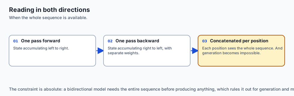
In many NLP tasks (like text classification, named entity recognition, or translation encoding), the model has access to the entire sequence at once:
- Bidirectional RNN (Schuster & Paliwal, 1997): Duplicates the recurrent layer into two independent streams:
- Forward RNN: Computes $\overrightarrow(h)t = \tanh(W(xh)^f x_t + W_(hh)^f \overrightarrow(h)_(t-1))$ from step $1$ to $T$.
- Backward RNN: Computes $\overleftarrow(h)t = \tanh(W(xh)^b x_t + W_(hh)^b \overleftarrow(h)_(t+1))$ from step $T$ down to $1$.
- Concatenated Representation: At every step $t$, the output vector is the concatenation $h_t = [\overrightarrow(h)_t ,;, \overleftarrow(h)_t] \in R^(2 d_h)$, giving every token full context of both past and future words.
6. Deep Stacked Recurrent Networks & Recurrent Dropout
To increase expressive capacity, multiple recurrent layers are stacked vertically:
-
In a $L$-layer RNN, the hidden state activations $h_t^((l-1))$ of layer $l-1$ serve as the input sequence to layer $l$:
h_t^{(l)} = tanh(W_{xh}^{(l)} h_t^{(l-1)} + W_{hh}^{(l)} h_{t-1}^{(l)} + b_h^{(l)}) -
Variational Recurrent Dropout (Gal & Ghahramani, 2016): Applying standard dropout to recurrent transitions destroys temporal memory. Variational dropout samples a single dropout mask at step $t=1$ and locks that exact mask across all time steps within the sequence.
7. Teacher Forcing vs Exposure Bias
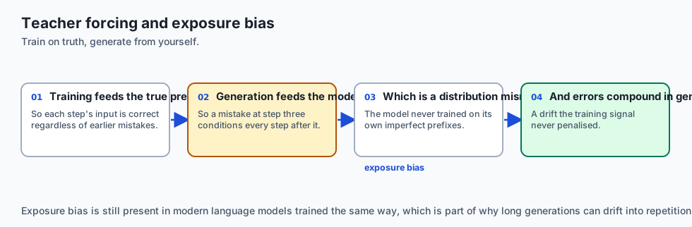
When training autoregressive sequence generators (e.g. character language models):
- Teacher Forcing: During training, the network receives the true ground-truth token $y_(t-1)^*$ as input at step $t$, regardless of what the network predicted at step $t-1$. This accelerates training convergence.
- Exposure Bias: At test time, ground truth is unavailable, so the network must feed its own (potentially flawed) previous prediction $\hat(y)_(t-1)$ back into step $t$. Errors compound over long generation steps.
- Scheduled Sampling (Bengio et al., 2015): Gradually transitions from Teacher Forcing to free-running autoregressive sampling during training.
8. Modern Linear Recurrence: From RNNs to Mamba (SSMs)
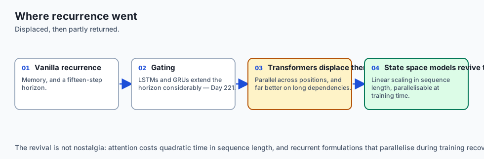
In 2023–2024, researchers revived recurrent principles with Selective State Space Models (Mamba / Gu & Dao):
-
Replaces non-linear $\tanh$ recurrences with linear time-invariant state equations ($h_t = A h_(t-1) + B x_t$), which can be computed as a parallel associative prefix scan on GPUs.
-
Achieves $O(N)$ linear inference speed with Transformer-quality long-context memory retention.
-
Hardware-Aware Memory Scans: Modern linear recurrent models bypass GPU memory bandwidth bottlenecks by fusing state updates into custom SRAM GPU kernels (Flash-Linear-Attention / Mamba CUDA kernel), eliminating VRAM round-trips.
An everyday analogy
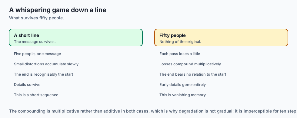
Think of a whispering game (Chinese Whispers / Telephone) played down a line of 50 people:
- Person 1 whispers a secret clue into Person 2’s ear.
- As the message passes from person to person (time steps), each person adds slight noise and forgets details (vanishing gradient).
- By the time Person 50 receives the message, the original clue has completely vanished.
- Conversely, if each person exaggerates and screams louder than the last (exploding gradient), the message turns into deafening screeching noise.
Examples in practice
Let us build a Vanilla RNN Cell from Scratch in PyTorch:
import torch
import torch.nn as nn
import torch.nn.functional as F

class CustomRNNCell(nn.Module):
    def __init__(self, input_dim: int, hidden_dim: int):
        super().__init__()
        self.input_dim = input_dim
        self.hidden_dim = hidden_dim

        # Input-to-hidden and Hidden-to-hidden weights
        self.W_xh = nn.Linear(input_dim, hidden_dim)
        self.W_hh = nn.Linear(hidden_dim, hidden_dim, bias=False)

    def forward(self, x_t: torch.Tensor, h_prev: torch.Tensor) -> torch.Tensor:
        # x_t: (Batch, input_dim)
        # h_prev: (Batch, hidden_dim)
        h_t = torch.tanh(self.W_xh(x_t) + self.W_hh(h_prev))
        return h_t

class VanillaRNN(nn.Module):
    def __init__(self, input_dim: int, hidden_dim: int, output_dim: int):
        super().__init__()
        self.hidden_dim = hidden_dim
        self.cell = CustomRNNCell(input_dim, hidden_dim)
        self.fc_out = nn.Linear(hidden_dim, output_dim)

    def forward(self, x: torch.Tensor, h_0: torch.Tensor = None) -> torch.Tensor:
        # x shape: (Batch, Seq_Len, input_dim)
        batch_size, seq_len, _ = x.size()

        if h_0 is None:
            h_t = torch.zeros(batch_size, self.hidden_dim, device=x.device)
        else:
            h_t = h_0

        # Unroll across time
        for t in range(seq_len):
            x_t = x[:, t, :]
            h_t = self.cell(x_t, h_t)

        # Output logits from final hidden state
        logits = self.fc_out(h_t)
        return logits
Implications: security, privacy, performance, scalability, and cost
- Sequential Compute Bottleneck on GPUs:
- Unlike CNNs and Transformers which process all tokens in parallel, RNNs are strictly bound by sequential data dependencies: step $t$ must wait for step $t-1$. This leads to poor GPU compute utilization and slow training speeds on long documents.
- Truncated BPTT in Production:
- When training RNNs on streaming audio or long texts, backpropagating over 10,000 steps exhausts GPU memory. Truncated BPTT splits sequences into windows of $k_1$ forward steps and $k_2$ backward steps, capping memory requirements.
Alternatives: free, open source, and commercial
| Architecture | Memory Span | Parallelizability | Best For |
|---|---|---|---|
| Vanilla RNN | Short (5 - 10 steps) | Sequential (Low) | Microcontroller / Low-latency simple signals |
| LSTM / GRU | Medium (100 - 500 steps) | Sequential (Low) | Classical NLP, speech, tabular time-series |
| 1D CNN (WaveNet) | Medium (Receptive field) | Fully Parallel | Fast audio waveform generation |
| Transformer / Mamba | Long / Infinite | Fully Parallel | Modern LLMs, long document reasoning |
Comparison with related concepts
┌────────────────────────────────────────────────────────────────────────┐
│                   SEQUENCE MODELING EVOLUTION                          │
├────────────────────┬─────────────────┬──────────────────┬──────────────┤
│ Architecture       │ State Mechanism │ Gradient Highway │ GPU Scaling  │
├────────────────────┼─────────────────┼──────────────────┼──────────────┤
│ Vanilla RNN        │ Single h_t      │ Vanishing (tanh) │ Sequential   │
│ LSTM               │ Hidden + Cell C │ Constant Carousel│ Sequential   │
│ GRU                │ Gated Single h  │ Gated Highway    │ Sequential   │
│ Transformer        │ Self-Attention  │ Residual Highway │ Fully Para   │
└────────────────────┴─────────────────┴──────────────────┴──────────────┘
When to use it — and when not to
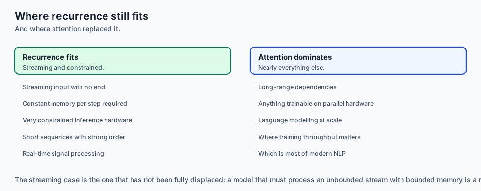
When to USE Vanilla RNNs:
- Lightweight embedded sensor time-series forecasting on tiny microcontrollers (ARM Cortex-M) with strict RAM limits (< 64 KB).
When NOT to use:
- Natural language generation, document classification, or machine translation where dependencies span across dozens of words (use LSTMs, Transformers, or State Space Models like Mamba).
The AI connection
- Recurrence was the first architecture with memory, and its sequential dependency is exactly what made it unable to use modern parallel hardware.
- The vanishing gradient over time is the same chain-rule product as over depth, with time steps in place of layers — which is why it bites after ten or fifteen steps.
- Teacher forcing creates exposure bias. The model trains on true prefixes and generates from its own, which is a distribution mismatch nobody removed until much later.
- The sequential bottleneck is why transformers won, not accuracy alone: attention computes every position at once and recurrence cannot.
- Recurrence returned as state space models, which recover linear scaling in sequence length while remaining parallelisable at training time.
Knowledge check
- What is the fundamental recurrence equation defining a simple Elman RNN cell?
- Why are weight matrices shared across all time steps during sequence processing?
- What causes the vanishing gradient problem during Backpropagation Through Time (BPTT)?
- How does L2 gradient norm clipping prevent numerical overflow during RNN training?
- What is the sequential execution bottleneck that makes RNNs slower to train on GPUs than Transformers?
Hands-on exercise
In this lab, you will build and test a custom Recurrent Neural Network (RNN) in PyTorch: implement the recurrent cell forward equation from first principles, construct a sequence unrolling loop, implement an automated Gradient Norm Clipping utility, train a many-to-one sequence classifier on synthetic time-series data, and verify gradient backpropagation stability.
Expected output
[Recurrent Neural Network Verification Suite]
Testing Custom RNN Cell & Forward Unrolling:
  Input Sequence Tensor Shape: torch.Size([16, 10, 8]) (Batch=16, Steps=10, Dim=8)
  Final Hidden State Shape:    torch.Size([16, 32])
  Output Logits Shape:         torch.Size([16, 2])
Testing Gradient Norm Clipping Controller:
  Original Gradient Norm:  14.82 [EXPLODING GRADIENT SIMULATED]
  Clipped Gradient Norm:   1.00  [BOUNDED TO THRESHOLD C=1.0]
Testing Sequence Classification Training Loop:
  Epoch 1/5: Loss = 0.6931 -> Epoch 5/5: Loss = 0.2104 [TRAINING CONVERGED]
Test Suite: 3 passed in 0.35s
Validate your work
Run the automated test runner:
./tests/run_tests.shTroubleshooting
- If gradients explode to
NaN, ensure you executetorch.nn.utils.clip_grad_norm_(model.parameters(), max_norm=1.0)immediately beforeoptimizer.step(). - Ensure initial hidden state $h_0$ is detached from previous graph iterations if training across truncated sequence windows.
Common mistakes
- Re-initializing Hidden State inside the Time Loop: Initializing $h = 0$ inside
for t in range(seq_len)turns the RNN into an MLP and destroys recurrent memory.
Practice assignment
- Implement a Bidirectional Vanilla RNN (BiRNN) that processes the input sequence forward ($1 \rightarrow T$) and backward ($T \rightarrow 1$), concatenating both hidden states at each step.
- Build a Character-Level Text Generator that samples characters one by one with temperature scaling from an RNN trained on Shakespeare’s sonnets.
Extension challenge
Implement Exact Manual Backpropagation Through Time (BPTT) in Pure NumPy:
- Write explicit analytical gradient equations for $\frac(\partial L)(\partial W_(xh))$, $\frac(\partial L)(\partial W_(hh))$, and $\frac(\partial L)(\partial W_(hy))$.
- Unroll the backward pass loop and verify gradient numerical equivalence against PyTorch
autograd.
Quiz
Q1. What is the core mathematical mechanism that distinguishes a Recurrent Neural Network (RNN) from a standard Feedforward Multilayer Perceptron (MLP)?
- RNNs only process images
- RNNs use two-dimensional convolutional kernels instead
- RNNs have no activation functions
- A hidden state carried and updated at every step
Show answer
Answer: D. A hidden state carried and updated at every step
Recurrent networks maintain a hidden state vector passed from step to step, allowing information to persist across sequential inputs.
Q2. Why are the weight matrices W_xh, W_hh, and W_hy shared (identical) across all sequential time steps in an unrolled RNN?
- Sharing weights handles any length with fixed parameters
- It prevents PyTorch from running out of RAM
- Because backpropagation cannot calculate gradients for different matrices
- It converts the network into a Transformer
Show answer
Answer: A. Sharing weights handles any length with fixed parameters
Parameter sharing across time enforces temporal equivariance and allows the model to process sequences of arbitrary lengths.
Q3. What is the primary cause of the Vanishing Gradient problem during Backpropagation Through Time (BPTT) in vanilla RNNs?
- The learning rate is too high
- Repeated multiplication by W_hh shrinks gradients
- The vocabulary size is too small
- Using float32 instead of float64
Show answer
Answer: B. Repeated multiplication by W_hh shrinks gradients
Repeated Jacobian matrix products over long temporal horizons cause gradients to vanish exponentially, preventing long-range dependency learning.
Q4. How does Gradient Norm Clipping prevent training divergence when encountering exploding gradients in RNNs?
- It stops training immediately
- It sets all of the negative gradients to zero instead
- It rescales the gradient when its norm exceeds C
- It reduces the batch size to 1
Show answer
Answer: C. It rescales the gradient when its norm exceeds C
Gradient clipping rescales the gradient vector proportionally when its total L2 norm exceeds threshold C, preserving the optimization descent direction.
Q5. Which sequence modeling topology is used when an RNN takes a variable-length paragraph as input and predicts a single binary sentiment label?
- Many-to-Many (Synchronized)
- One-to-One
- One-to-Many
- Many-to-one, reading the final hidden state
Show answer
Answer: D. Many-to-one, reading the final hidden state
Many-to-one processes a full input sequence and uses the final time step hidden state for global sequence classification.
Glossary
- Recurrent Neural Network (RNN)
- A class of neural networks where connections between nodes form a directed cycle along a temporal sequence, enabling internal memory states.
- Hidden State
- A continuous vector (h_t) serving as the sequential memory buffer updated at each time step based on current input and past hidden state.
- Backpropagation Through Time (BPTT)
- The algorithm that unrolls an RNN across sequential time steps and applies the chain rule backward from the final loss to early steps.
- Vanishing Gradient Problem
- The exponential decay of error gradients as they backpropagate across multiple recurrent time steps, preventing long-range dependency learning.
- Exploding Gradient Problem
- The exponential growth of error gradients across time steps, causing catastrophic numerical overflow and model divergence.
- Gradient Norm Clipping
- A regularization technique that rescales gradient vectors whose L2 norm exceeds a maximum threshold C to prevent optimization instability.
- Truncated BPTT
- An engineering practice of splitting long sequences into chunks of k time steps, limiting backpropagation depth to bound compute and memory.
- Temporal Equivariance
- The mathematical property ensuring that a sequential pattern is processed identically regardless of its absolute timestamp in the sequence.
Sources and further reading
- Finding Structure in Time — Cognitive Science (accessed 2026-08-29)
- Learning Long-Term Dependencies with Gradient Descent is Difficult — IEEE Transactions on Neural Networks (accessed 2026-08-29)
- On the Difficulty of Training Recurrent Neural Networks — ICML 2013 (accessed 2026-08-29)
Kept in this browser, no account needed. Your progress page turns the whole record into one link you can bookmark or open on another device.