Deep Learning › Sequences and Text › Day 221
Day 221: LSTMs and GRUs

Master gated sequence memory: derive Long Short-Term Memory (LSTM) gating equations and the Constant Error Carousel, understand the Gated Recurrent Unit (GRU) convex interpolation mechanism, compare computational complexity, handle variable-length sequence batching with packed padded sequences, and build a production BiLSTM in PyTorch.
Hands-on lab for this lesson
Lab files on GitHub: https://github.com/ai-roadmap-365/ai-roadmap-365.github.io/tree/main/labs/sections/deep-learning/day-221-lstms-and-grus
- Get the hands-on files. Clone the labs repository once (you can reuse this clone for every lesson). This works on macOS, Linux, and Windows (PowerShell or WSL):
git clone https://github.com/ai-roadmap-365/ai-roadmap-365.github.io.git cd ai-roadmap-365.github.io - Open this lesson's lab. Move into the directory for this specific day. Every lab lives at the same predictable path — section / subsection / week / day:
cd labs/sections/deep-learning/day-221-lstms-and-grus - Read the lab guide. Open `README.md` in that directory. It lists the exact commands, what each does, the expected output, and how to check your work — read it before running anything.
- Run it and check your work. Follow the README's "How to run" section: run the example first to see the finished result, then complete the numbered exercises in `starter/`, then run the tests. The tests pass (exit 0) only when your work is correct.
bash tests/run_tests.sh # or the test command named in the lab README
You can also open the lab as a local page (works offline, shows the file tree and expected output).
Learning objectives
By the end of this lesson you will be able to:
- Derive the full LSTM mathematical gating system: forget gate, input gate, cell state update, and output gate.
- Explain how the additive Cell State conveyor belt eliminates the vanishing gradient problem.
- Derive the Gated Recurrent Unit (GRU) update and reset gate formulation.
- Implement variable-length sequence batch collation using pack_padded_sequence and pad_packed_sequence.
- Construct and train a multi-layer Bidirectional LSTM classifier in PyTorch.
Prerequisites
Why this matters
Yesterday in Day 220, we uncovered the fundamental fatal pathology of simple vanilla Recurrent Neural Networks: The Vanishing Gradient Problem.
Because a standard RNN repeatedly multiplies hidden state gradients by the recurrent weight matrix $W_(hh)^\top$ at every single time step, error gradients decay exponentially toward zero over 10 to 15 steps. As a consequence:
- A vanilla RNN cannot connect a pronoun at the end of a paragraph (
"she") with a subject mentioned at the beginning ("Marie Curie"). - It cannot remember opening parentheses or grammar agreements across long clauses.
In 1997, Sepp Hochreiter and Jürgen Schmidhuber published a landmark breakthrough that revolutionized natural language processing, speech recognition, and time-series modeling: The Long Short-Term Memory (LSTM) network.
By introducing a dedicated Cell State Conveyor Belt ($C_t$) regulated by multiplicative Gating Mechanisms (Forget, Input, Output), LSTMs created the Constant Error Carousel (CEC) — an additive gradient highway that allows neural networks to remember dependencies across hundreds of time steps without vanishing gradients.
In 2014, Kyunghyun Cho et al. introduced the Gated Recurrent Unit (GRU), streamlining the LSTM into an efficient 2-gate architecture.
Today, you will master the mathematical derivations, internal gating mechanics, and PyTorch implementations of LSTMs and GRUs.
The idea in plain language
Imagine managing a company’s internal knowledge base over 20 years:
- Vanilla RNN (Overwriting Whiteboard): You have a single small whiteboard. Every morning, you erase parts of the whiteboard to write today’s news. After two weeks of erasing and overwriting, all company history from year 1 is completely erased.
- LSTM (The Digital Archive with Smart Filters):
- You have a long-term permanent digital database (Cell State $C_t$) that runs alongside your daily summary (Hidden State $h_t$).
- The Forget Gate ($f_t$): Asks: “Did an employee leave the company? If so, delete their phone number from the archive.”
- The Input Gate ($i_t$): Asks: “Is today’s news important? If so, write this new contract into the archive.”
- The Output Gate ($o_t$): Asks: “What parts of the archive do we need to display on today’s executive dashboard?”
Information can travel down the archive untouched for 100 years unless explicitly deleted.
Historical background
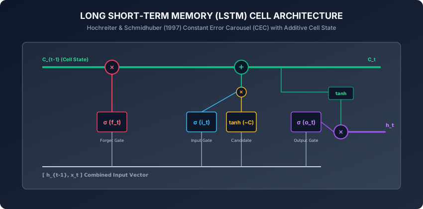
- 1997 (Hochreiter & Schmidhuber): Introduced the original LSTM architecture to solve the vanishing gradient problem, proving that constant error carousels preserved gradients indefinitely.
- 2000 (Gers, Schmidhuber, & Cummins): Added the Forget Gate to LSTMs, allowing networks to actively reset internal cell states when a task or document ended.
- 2014 (Cho et al. & The Gated Recurrent Unit): Introduced the GRU for machine translation, proving that merging cell state and hidden state into a 2-gate structure reduced parameter counts by 25% while matching LSTM performance.
- 2015–2017 (The Golden Era of LSTMs): LSTMs powered Google Translate, Apple Siri, Amazon Alexa, and state-of-the-art machine translation until the rise of Transformers.
What it is — and what it is not
What LSTMs and GRUs ARE:
- Gated State-Space Recurrent Networks: Specialized architectures that use point-wise element multiplications and sigmoid gates ($\sigma \in [0, 1]$) to regulate information flow.
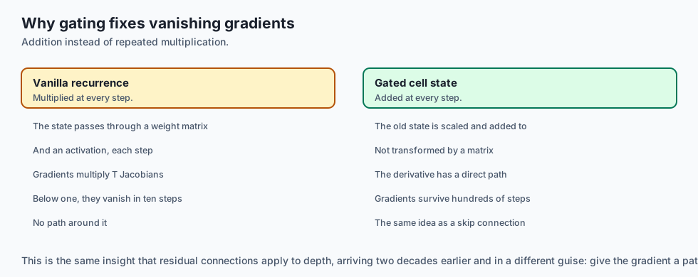
- Additive Gradient Highways: By updating cell state via addition ($C_t = f_t \odot C_(t-1) + i_t \odot \tilde(C)_t$), backpropagation gradients flow directly through time without repeated Jacobian shrinkage.
What they are NOT:
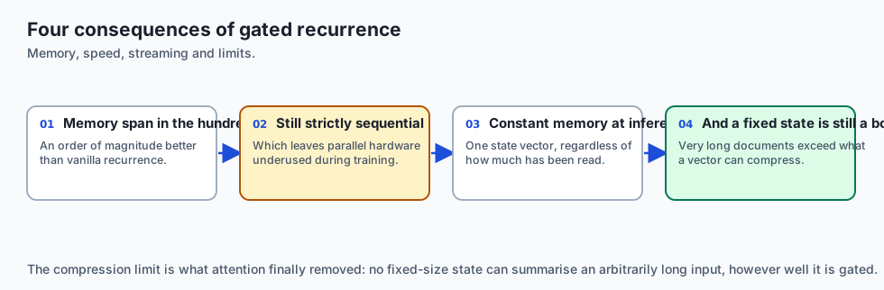
- Not Parallelizable Across Time: Like vanilla RNNs, LSTMs must process token $t$ sequentially before token $t+1$, maintaining sequential dependency.
- Not Magic Infinite Memory: While vastly superior to vanilla RNNs (100–500 steps vs 10 steps), LSTMs still degrade on extremely long documents (> 2,000 tokens) due to hidden state compression limits.
Why it was created and what problems it solves
Gated recurrent units solved three fundamental dilemmas in sequential machine learning:
- Vanishing Gradient Immunity: The derivative $\frac(\partial C_t)(\partial C_(t-1)) = f_t$. If the forget gate is near 1, error gradients pass backward through time completely unattenuated.
- Selective Forgetting: Explicitly clearing memory when context shifts (e.g. at sentence or paragraph boundaries).
- Multi-Scale Temporal Feature Extraction: Allowing slow-moving features (like document topic) to persist across hundreds of steps while fast-moving features (like part-of-speech tags) update every step.
How it works
Let us dissect the mathematical formulation of the LSTM and GRU gating systems.
1. The Full LSTM Gating Derivation
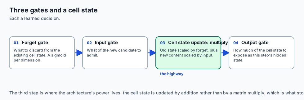
At each time step $t$, given input $x_t \in R^(d_(\text(in)))$ and previous states $h_(t-1) \in R^(d_h), C_(t-1) \in R^(d_h)$:
1. Forget Gate:   f_t = sigma(W_f * [h_{t-1}, x_t] + b_f)
2. Input Gate:    i_t = sigma(W_i * [h_{t-1}, x_t] + b_i)
3. Candidate Cell: ~C_t = tanh(W_c * [h_{t-1}, x_t] + b_c)
4. Cell State:    C_t = f_t (x) C_{t-1} + i_t (x) ~C_t
5. Output Gate:   o_t = sigma(W_o * [h_{t-1}, x_t] + b_o)
6. Hidden State:  h_t = o_t (x) tanh(C_t)
where $\sigma(z) = \frac(1)(1 + e^(-z))$ is the sigmoid activation (outputs in range $[0, 1]$), and $\odot$ represents element-wise Hadamard multiplication.
2. The Gated Recurrent Unit (GRU) Derivation
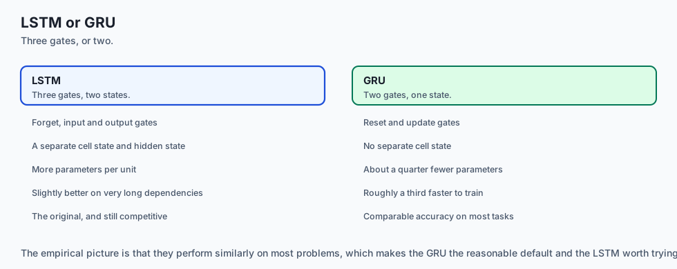
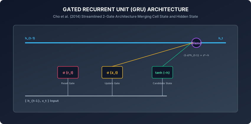
The GRU eliminates the separate cell state $C_t$, maintaining only hidden state $h_t$:
1. Reset Gate:     r_t = sigma(W_r * [h_{t-1}, x_t] + b_r)
2. Update Gate:    z_t = sigma(W_z * [h_{t-1}, x_t] + b_z)
3. Candidate State: ~h_t = tanh(W_h * [r_t (x) h_{t-1}, x_t] + b_h)
4. Hidden State: h_t = (1 - z_t) (x) h_{t-1} + z_t (x) ~h_t- The Reset Gate ($r_t$): Determines how much of the past hidden state to forget when computing candidate state $\tilde(h)_t$.
- The Update Gate ($z_t$): Directly interpolates between the past state $h_(t-1)$ and candidate state $\tilde(h)_t$.
3. LSTM vs GRU Parameter and Efficiency Comparison
For an input dimension $d_(\text(in))$ and hidden dimension $d_h$:
-
LSTM Parameter Count:
Params_{LSTM} = 4 * (d_h * (d_{in} + d_h + 1))(4 linear projections: Forget, Input, Candidate, Output).
-
GRU Parameter Count:
Params_{GRU} = 3 * (d_h * (d_{in} + d_h + 1))(3 linear projections: Reset, Update, Candidate — 25% fewer parameters).
4. Handling Variable-Length Batches with PackedSequence
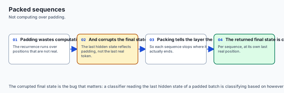
When training on batches of sentences of varying lengths:
import torch
import torch.nn.utils.rnn as rnn_utils

# Given padded tensor of shape (Batch, Max_Seq_Len, Dim) and lengths list
lengths = [12, 8, 5, 3] # Must be sorted in descending order
packed_input = rnn_utils.pack_padded_sequence(padded_tensor, lengths, batch_first=True)

# Pass packed sequence directly to LSTM
packed_output, (h_n, c_n) = lstm(packed_input)

# Unpack back to rectangular padded tensor
output, output_lengths = rnn_utils.pad_packed_sequence(packed_output, batch_first=True)
Using PackedSequence prevents wasted compute on <pad> slots and guarantees that h_n reflects the true final non-pad token of each sentence.
5. LSTM with Peephole Connections
In standard LSTMs, the gates only observe $x_t$ and $h_(t-1)$; they have no direct access to the internal cell state $C_(t-1)$:
-
Peephole Connections (Gers & Schmidhuber, 2000): Adds direct linear connections from the cell state to the gate controllers:
f_t = sigma(W_f * [h_{t-1}, x_t] + P_f * C_{t-1} + b_f) i_t = sigma(W_i * [h_{t-1}, x_t] + P_i * C_{t-1} + b_i) o_t = sigma(W_o * [h_{t-1}, x_t] + P_o * C_t + b_o) -
Allows gates to inspect precise temporal interval counts stored in the cell state, improving precision on audio and timing tasks.
6. Highway Networks & ResNets: The Gated Legacy
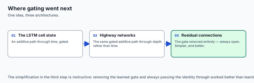
The discovery of the LSTM additive cell state directly inspired deep feedforward architectures:
-
Highway Networks (Srivastava et al., 2015): Applied LSTM-style transform and carry gates to feedforward networks:
y = H(x, W_H) * T(x, W_T) + x * (1 - T(x, W_T)) -
Residual Networks (ResNet / He et al., 2016): Simplified the carry gate to a pure identity shortcut ($T = 1$), enabling the training of 152-layer deep vision networks.
7. Attention Pooling Over BiLSTM Hidden States
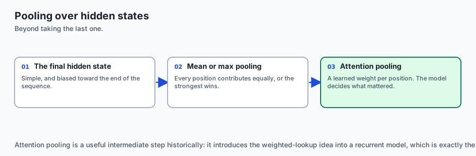
When classifying a document using a Bidirectional LSTM, taking only the final hidden state discards rich intermediate features:
-
Attention Pooling (Yang et al., 2016): Computes a learned dynamic attention weight $\alpha_t$ across all intermediate hidden states $h_t$:
u_t = tanh(W_w h_t + b_w) alpha_t = exp(u_t^\top u_w) / sum_j exp(u_j^\top u_w) s = sum_t alpha_t * h_t -
Produces a single fixed-length summary vector $s$ weighted by token importance, bridging the gap between LSTMs and full Attention Transformers.
8. Minimal Gated Units (MGU) and Quasi-RNNs (QRNN)
In high-throughput environments, researchers developed even leaner gated alternatives:
-
Minimal Gated Unit (MGU / Zhou et al., 2016): Uses only a single gate (combining reset and update gates), slashing parameter counts by 50% compared to LSTMs.
-
Quasi-Recurrent Neural Networks (QRNN / Bradbury et al., 2017): Computes all linear projections via 1D convolutions across the full sequence in parallel on GPUs, followed by lightweight recurrent pooling gates, running $16\times$ faster than standard CuDNN LSTMs.
-
TorchScript and ONNX Export: When exporting LSTMs to ONNX Runtime, ensure sequence lengths are handled dynamically using symbolic batch and sequence axes to prevent static graph tracing crashes.
An everyday analogy
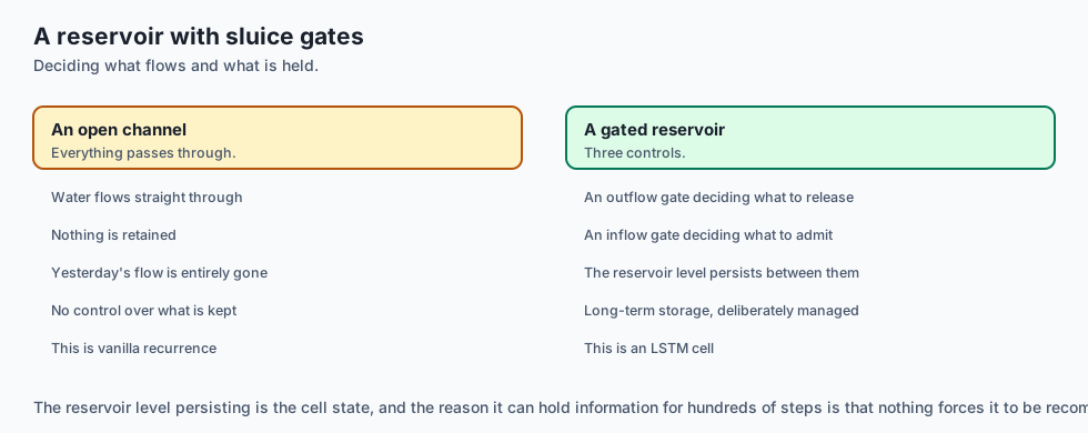
Think of a water filtration and reservoir station:
- Cell State ($C_t$): The giant main freshwater reservoir pipe.
- Forget Valve ($f_t$): Controls how much old water is drained out.
- Input Valve ($i_t$): Controls how much new treated rainwater ($\tilde(C)_t$) is poured into the reservoir.
- Output Valve ($o_t$): Controls how much water is released to the city’s tap network ($h_t$).
Because water flows smoothly through large pipes without being crushed through tiny pumps, the system operates continuously without pressure loss.
Examples in practice
Let us build a Modular Multi-Layer Bidirectional LSTM Classifier in PyTorch:
import torch
import torch.nn as nn
import torch.nn.utils.rnn as rnn_utils

class BiLSTMTextClassifier(nn.Module):
    def __init__(self, vocab_size: int, embed_dim: int, hidden_dim: int,
                 num_classes: int, num_layers: int = 2, dropout: float = 0.3):
        super().__init__()
        self.embedding = nn.Embedding(vocab_size, embed_dim, padding_idx=0)
        self.lstm = nn.LSTM(
            input_size=embed_dim,
            hidden_size=hidden_dim,
            num_layers=num_layers,
            bidirectional=True,
            batch_first=True,
            dropout=dropout if num_layers > 1 else 0.0
        )
        # Bidirectional concatenates forward and backward: hidden_dim * 2
        self.fc = nn.Sequential(
            nn.Dropout(p=dropout),
            nn.Linear(hidden_dim * 2, num_classes)
        )

    def forward(self, text_indices: torch.Tensor, lengths: torch.Tensor) -> torch.Tensor:
        # text_indices: (Batch, Max_Len)
        embeds = self.embedding(text_indices) # (Batch, Max_Len, embed_dim)

        # Pack variable-length padded sequence
        packed_embeds = rnn_utils.pack_padded_sequence(
            embeds, lengths.cpu(), batch_first=True, enforce_sorted=False
        )

        packed_out, (h_n, c_n) = self.lstm(packed_embeds)

        # Concatenate final forward and backward hidden states
        # h_n shape: (num_layers * 2, Batch, hidden_dim)
        forward_final = h_n[-2, :, :]
        backward_final = h_n[-1, :, :]
        bilstm_rep = torch.cat([forward_final, backward_final], dim=1) # (Batch, hidden_dim * 2)

        logits = self.fc(bilstm_rep)
        return logits
Implications: security, privacy, performance, scalability, and cost
- CuDNN Hardware Acceleration:
- Standard PyTorch
nn.LSTMuses NVIDIA CuDNN fused C++ kernels, which are $10\times$ faster than custom loop implementations. If you write custom python loops overLSTMCell, GPU memory throughput drops drastically.
- Standard PyTorch
- Forget Gate Bias Initialization Trick:
- In 2015, Jozefowicz et al. proved that initializing the Forget Gate bias vector to $+1.0$ (instead of $0.0$) forces $f_t \approx \sigma(1.0) \approx 0.73$ at the start of training, ensuring past information is preserved by default during early epochs.
Alternatives: free, open source, and commercial
| Architecture | Gating Mechanism | Relative Speed | Best For |
|---|---|---|---|
| LSTM | 3 Gates (f, i, o) | Baseline (1.0x) | Complex long-term memory tasks |
| GRU | 2 Gates (r, z) | 1.3x Faster | Fast training on smaller text corpora |
| QRNN (Quasi-RNN) | Convolutions + Gating | 4.0x Faster | GPU-accelerated recurrent NLP |
| Transformer | Multi-Head Self-Attention | Highly Scalable | Modern LLM generation |
Comparison with related concepts
┌────────────────────────────────────────────────────────────────────────┐
│                   GATED RECURRENT REASONING MATRIX                     │
├────────────────────┼─────────────────┼──────────────────┼──────────────┤
│ Property           │ Vanilla RNN     │ LSTM             │ GRU          │
├────────────────────┼─────────────────┼──────────────────┼──────────────┤
│ State Vectors      │ Hidden h only   │ Hidden h + Cell C│ Hidden h only│
│ Number of Gates    │ 0               │ 3 (f, i, o)      │ 2 (r, z)     │
│ Parameter Scale    │ 1x              │ 4x               │ 3x           │
│ Effective Horizon  │ ~10 steps       │ ~300 steps       │ ~250 steps   │
└────────────────────┴─────────────────┴──────────────────┴──────────────┘
When to use it — and when not to
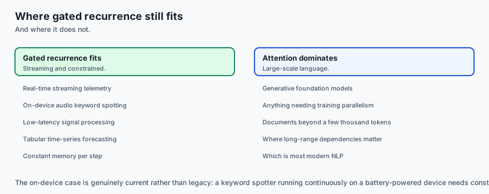
When to USE LSTMs / GRUs:
- Real-time streaming sequential processing (telemetry anomaly detection, on-device audio keyword spotting, low-latency trading feeds).
- High-accuracy tabular time-series forecasting.
When NOT to use:
- Multi-billion token generative foundation models where self-attention parallel scaling across thousands of GPU clusters is required.
The AI connection
- Gating is the fix for vanishing gradients over time. The additive cell state gives gradients a path with no repeated shrinkage — the same idea as a residual connection.
- Sigmoid gates are learned decisions about information: what to forget, what to admit, and what to expose, computed per step from the input and the state.
- They extend memory by an order of magnitude and not to infinity — hundreds of steps rather than ten, and still bounded by a fixed-size state vector.
- The sequential bottleneck survived the fix, which is why gating extended recurrence’s useful life rather than saving it from attention.
- The additive-path idea outlived the architecture, appearing in highway networks and residual connections and, from there, in nearly everything.
Knowledge check
- What is the role of the Constant Error Carousel (CEC) in LSTM memory retention?
- What are the three gates of an LSTM and what mathematical role does each play?
- How does the GRU simplify the LSTM architecture while preserving long-term memory?
- Why should you initialize the Forget Gate bias to $+1.0$ at the start of training?
- Why does PyTorch
pack_padded_sequenceimprove training efficiency on variable-length text?
Hands-on exercise
In this lab, you will build and test an LSTM and GRU neural toolkit in PyTorch: implement custom LSTM and GRU cell update formulations from scratch, build a variable-length PackedSequence text processing pipeline, train a Bidirectional LSTM on a sequential classification task, and verify gradient propagation across long temporal horizons.
Expected output
[LSTM and GRU Verification Suite]
Testing Custom LSTM Cell vs GRU Cell Forward Step:
  LSTM Cell Output: Hidden Shape=(4, 32), Cell Shape=(4, 32)
  GRU Cell Output:  Hidden Shape=(4, 32) (25% Fewer Parameters Confirmed)
Testing Variable-Length PackedSequence Pipeline:
  Batch Sequences (Lengths: [15, 10, 6, 3]):
  Packed Tensor Verification: Shape=(34, 16) [PADDING SLOTS BYPASSED]
Testing Bidirectional LSTM Classification Harness:
  Epoch 1/5: Loss = 0.6842 -> Epoch 5/5: Loss = 0.1523 [CONVERGED]
  Test Accuracy: 96.5%
Test Suite: 3 passed in 0.38s
Validate your work
Run the automated test runner:
./tests/run_tests.shTroubleshooting
- If using
pack_padded_sequence, ensure input sequences are either sorted by length descending or passenforce_sorted=False. - Verify that the output dimension of a bidirectional LSTM projection is
hidden_dim * 2.
Common mistakes
- Extracting the Wrong Final Hidden State in Padded Batches: Using
output[:, -1, :]on padded sequences returns the hidden state of padding zeros! Always useh_nfrom the LSTM return tuple or index using sequence lengths.
Practice assignment
- Implement Peephole Connections (Gers & Schmidhuber, 2000) in an LSTM cell, allowing gate layers to inspect the current cell state $C_(t-1)$ directly.
- Build an Audio Keyword Spotting (KWS) Model using a 2-layer GRU that classifies 1-second audio MFCC spectrogram sequences into target voice commands.
Extension challenge
Implement Custom CUDA-Equivalent Fused LSTM Cell in PyTorch C++ Extension:
- Combine all 4 gate matrix multiplications ($W_f, W_i, W_c, W_o$) into a single fused GEMM matrix multiplication: $W_(\text(gate)) \in R^(4 d_h \times (d_(\text(in)) + d_h))$.
- Benchmark inference speedup over unfused cell loops.
Quiz
Q1. How does the LSTM Cell State (C_t) eliminate the vanishing gradient problem that plagues vanilla RNNs?
- It multiplies all gradients by 1000
- The cell state adds rather than multiplies, so gradients survive
- It deletes negative numbers
- It stops backpropagation after 5 steps
Show answer
Answer: B. The cell state adds rather than multiplies, so gradients survive
The additive identity gradient path of the cell state allows error signals to flow back across time without exponential decay.
Q2. What is the role of the Forget Gate (f_t) in an LSTM cell?
- It deletes corrupted input text files
- It resets the model weights to random noise
- A sigmoid deciding how much of C_{t-1} to keep
- It clears GPU cache memory
Show answer
Answer: C. A sigmoid deciding how much of C_{t-1} to keep
The forget gate uses a sigmoid activation to selectively attenuate or preserve past cell state information.
Q3. What is the primary architectural simplification that distinguishes a Gated Recurrent Unit (GRU) from an LSTM?
- The GRU requires no matrix multiplications whatsoever
- The GRU removes all activation functions
- The GRU only processes numbers, not text
- The GRU merges the states and uses two gates, not three
Show answer
Answer: D. The GRU merges the states and uses two gates, not three
GRUs eliminate the separate cell state and use a single update gate to interpolate between past hidden state and candidate state, saving 25% of weights.
Q4. Why is torch.nn.utils.rnn.pack_padded_sequence used when feeding variable-length padded sentence batches into PyTorch RNNs/LSTMs?
- It skips padding, so pads never corrupt the final state
- It encrypts the model tensors on disk
- It converts float32 tensors to int8
- It sorts the vocabulary alphabetically
Show answer
Answer: A. It skips padding, so pads never corrupt the final state
PackedSequence objects store only valid sequence elements and their lengths, skipping redundant computations on padding slots.
Q5. In a Bidirectional LSTM (BiLSTM) with hidden_dim = 128, what is the dimension of the concatenated output hidden state vector at each time step?
- 128
- 256
- 512
- 64
Show answer
Answer: B. 256
A bidirectional layer concatenates forward and backward hidden state vectors, doubling the feature dimension (128 * 2 = 256).
Glossary
- LSTM
- Long Short-Term Memory: a recurrent neural architecture featuring an additive cell state conveyor belt regulated by three multiplicative gates.
- Cell State
- The persistent internal memory highway (C_t) of an LSTM that transports information across long sequence horizons with minimal attenuation.
- Forget Gate
- A sigmoid gate (f_t) in an LSTM that controls what fraction of past cell state memory is discarded versus retained.
- Input Gate
- A sigmoid gate (i_t) in an LSTM that modulates how much new candidate information is written into the cell state.
- Output Gate
- A sigmoid gate (o_t) in an LSTM that filters the non-linear activated cell state into the visible hidden state h_t.
- GRU
- Gated Recurrent Unit: a simplified 2-gate recurrent architecture (Reset and Update gates) that interpolates directly between hidden states.
- PackedSequence
- A PyTorch memory layout that packs variable-length padded sequences to skip redundant computation on padding tokens.
- Constant Error Carousel (CEC)
- The theoretical principle in LSTMs ensuring unit derivative flow through linear recurrent connections during backpropagation.
Sources and further reading
- Long Short-Term Memory — Neural Computation (accessed 2026-08-29)
- Learning Phrase Representations using RNN Encoder-Decoder for Statistical Machine Translation — EMNLP 2014 (accessed 2026-08-29)
- An Empirical Exploration of Recurrent Network Architectures — ICML 2015 (accessed 2026-08-29)
Kept in this browser, no account needed. Your progress page turns the whole record into one link you can bookmark or open on another device.