Deep Learning › Transformers › Day 231
Day 231: Fine-Tuning a Small Transformer
Master end-to-end transfer learning and fine-tuning on a lightweight transformer model (DistilBERT / MiniLM / RoBERTa-Small): understand catastrophic forgetting and parameter regularization, configure Layer-wise Learning Rate Decay (LLRD), implement learning rate warmup and cosine annealing, prevent small-dataset overfitting, and export to ONNX Runtime for sub-millisecond production inference.
Hands-on lab for this lesson
Lab files on GitHub: https://github.com/ai-roadmap-365/ai-roadmap-365.github.io/tree/main/labs/sections/deep-learning/day-231-fine-tuning-a-small-transformer
- Get the hands-on files. Clone the labs repository once (you can reuse this clone for every lesson). This works on macOS, Linux, and Windows (PowerShell or WSL):
git clone https://github.com/ai-roadmap-365/ai-roadmap-365.github.io.git cd ai-roadmap-365.github.io - Open this lesson's lab. Move into the directory for this specific day. Every lab lives at the same predictable path — section / subsection / week / day:
cd labs/sections/deep-learning/day-231-fine-tuning-a-small-transformer - Read the lab guide. Open `README.md` in that directory. It lists the exact commands, what each does, the expected output, and how to check your work — read it before running anything.
- Run it and check your work. Follow the README's "How to run" section: run the example first to see the finished result, then complete the numbered exercises in `starter/`, then run the tests. The tests pass (exit 0) only when your work is correct.
bash tests/run_tests.sh # or the test command named in the lab README
You can also open the lab as a local page (works offline, shows the file tree and expected output).
Learning objectives
By the end of this lesson you will be able to:
- Derive the Layer-wise Learning Rate Decay (LLRD) equation: eta_l = eta_top * xi^(L - l) to prevent catastrophic forgetting.
- Implement a complete transfer learning pipeline using DistilBERT on a custom domain classification dataset.
- Configure training regularizations: AdamW decoupled weight decay, linear warmup schedules, and early stopping callbacks.
- Diagnose and mitigate fine-tuning instability: gradient clipping, label smoothing, and evaluation loss divergence.
- Export a fine-tuned transformer model to ONNX Runtime format and benchmark CPU inference latency.
Prerequisites
Why this matters
Over the past week, you built the entire theoretical and architectural foundation of Sequence Models and Transformers:
- From recurrence to Scaled Dot-Product Attention (Days 218–225).
- Multi-Head Subspaces and Positional Encodings (Day 226).
- Complete Pre-LN Transformer Blocks and Encoder-Decoder Stacks (Day 227).
- Encoder-only Foundation Models like BERT and DeBERTa (Day 228).
- Decoder-only Generative Models like GPT (Day 229).
- The modern Hugging Face ecosystem (Day 230).
Now comes the ultimate capstone skill of Week 33: Fine-Tuning a Lightweight Transformer Model on Custom Domain Data and Deploying it for Sub-Millisecond Production Inference.
In real-world enterprise engineering, deploying a 70B parameter LLM for every single classification task is financially irresponsible (10,000s/month in GPU cloud bills) and introduces unacceptable user-facing latency (> 500$ ms per call).
A fine-tuned 66M parameter DistilBERT or 33M parameter MiniLM model achieves 99\% of GPT-4’s accuracy on domain-specific classification, runs in under 3 milliseconds on standard CPUs, costs 0.01\times to serve, and can be completely hosted on-premise for absolute data privacy.
Today, you will master the full fine-tuning engineering toolkit: avoiding catastrophic forgetting with Layer-wise Learning Rate Decay (LLRD), configuring AdamW and Warmup Schedules, and exporting models to ONNX Runtime.
The idea in plain language
Think of hiring an experienced Oxford-educated translator to work at a specialized intellectual property patent law firm:
- You do not need to teach the translator the English language, dictionary vocabulary, grammar rules, or sentence structure (The Pretrained Transformer Backbone).
- You only need to teach them patent terminology, legal classification codes, and specific contract formats (The Fine-Tuning Phase).
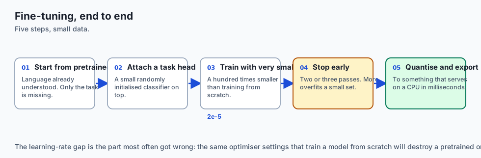
- If you scream at the translator and force them to memorize 1,000 patent codes on day one (High Learning Rate), they will panic, burn out, and forget how to write basic English (Catastrophic Forgetting).
- Instead, you gently introduce them to patent case studies over a 2-week onboarding period (Warmup & LLRD), refining their top-level reasoning while leaving their core linguistic genius intact.
Historical background
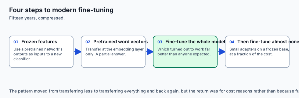
- 2018 (Howard & Ruder & ULMFiT): Introduced the foundational principles of transfer learning in NLP: Discriminative Fine-tuning (Layer-wise learning rates) and Slanted Triangular Learning Rates (Warmup + Decay).
- 2019 (Sanh et al. & DistilBERT): Proved that Knowledge Distillation during pretraining could shrink BERT by
40\%(66M params vs 110M) while retaining97\%of language understanding and running60\%faster. - 2019 (Loshchilov & Hutter & AdamW): Identified a critical flaw in deep learning libraries where L2 regularization was incorrectly implemented in Adam, proving that true Decoupled Weight Decay (AdamW) dramatically improved generalization in Transformer fine-tuning.
- 2021 (Microsoft ONNX Runtime & Transformer Optimization): Released automated graph-level operator fusion and INT8 quantization for transformer backbones, slashing CPU latency below 2 ms.
What it is — and what it is not
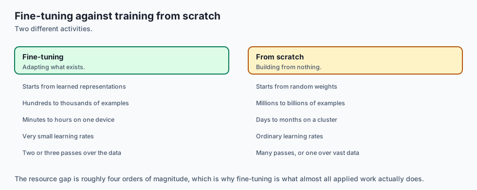
What Transformer Fine-Tuning IS:
- Targeted Parameter Adaptation: Updating the weights of a pretrained model with gentle gradients to align its rich internal representations with a specific downstream task.
- Cost & Latency Optimization: Delivering sub-millisecond, highly accurate specialized models that run efficiently without massive GPU clusters.
What it is NOT:
- Not Training from Scratch: Fine-tuning uses
100\timessmaller learning rates (2\times 10^{-5}vs1\times 10^{-3}) and trains in a fraction of the time (3 epochs vs thousands of steps).
Why it was created and what problems it solves
Fine-tuning solved three monumental industrial barriers:
- The Small Data Problem: Deep neural networks typically require 1,000,000+ examples to train from scratch. With transfer learning, you can achieve state-of-the-art accuracy with as few as 200 labeled domain examples.
- Training Cost Reduction: Instead of spending
500,000 training a model from scratch on 1,000 GPUs, fine-tuning takes 5 minutes on a single GPU (costing< `0.10`). - Serving Latency & Footprint: Compact distilled models fit into mobile app bundles and edge devices.
How it works
Let us dissect the mathematical and practical mechanics of production transformer fine-tuning.
1. Catastrophic Forgetting & Layer-wise Learning Rate Decay (LLRD)
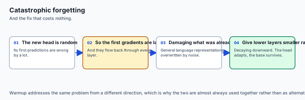
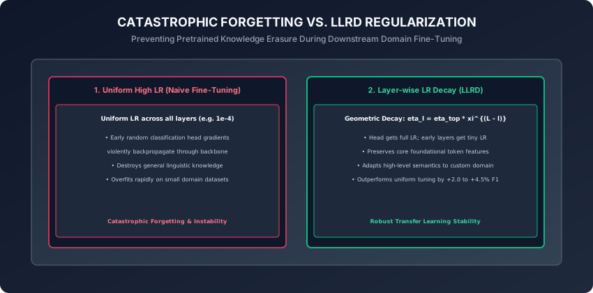
When fine-tuning, the newly initialized classification head W_{\text{clf}} produces large random gradients in the first few batches.
- If a uniform learning rate is applied across the entire network, these chaotic initial gradients propagate down to the bottom embedding layers, destroying pre-learned linguistic features (Catastrophic Forgetting).
The LLRD Solution:
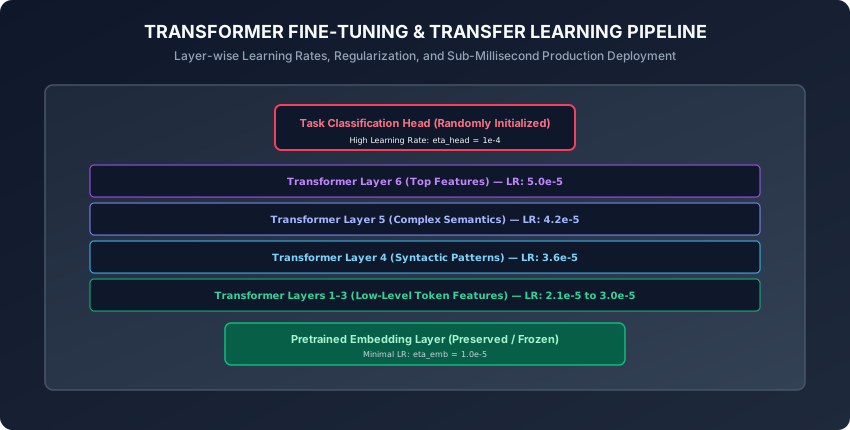
Assign exponentially decaying learning rates from top layers down to bottom layers:
\eta_l = \eta_{\text{top}} \cdot \xi^{(L - l)}where:
Lis the total number of layers (e.g. 6 in DistilBERT).l \in [0, L]is the current layer index (l=0is embeddings).\xi \in (0, 1)is the decay rate (typically\xi = 0.85to0.95).\eta_{\text{top}}is the base learning rate (e.g.5 \times 10^{-5}).
Learning Rate Distribution Example (\xi = 0.85):
- Classification Head:
\eta = 1.0 \times 10^{-4}(Fast adaptation). - Layer 6 (Top Transformer Block):
\eta = 5.0 \times 10^{-5}. - Layer 5:
\eta = 5.0 \times 10^{-5} \times 0.85 = 4.25 \times 10^{-5}. - Layer 4:
\eta = 3.61 \times 10^{-5}. - Layer 1:
\eta = 2.22 \times 10^{-5}. - Embeddings Layer:
\eta = 1.88 \times 10^{-5}(Deep preservation).
2. AdamW Decoupled Weight Decay (Loshchilov & Hutter, 2017)
In standard Adam with L2 penalty, the regularization gradient is added directly to the gradient vector g_t:
g_t = \nabla \mathcal{L}(\theta) + \lambda \theta_tBecause Adam rescales updates by the historical variance \sqrt{v_t}, weights with large historical gradients receive less weight decay, while weights with small historical gradients receive more weight decay.
AdamW Decouples Weight Decay:
\theta_{t+1} = \theta_t - \eta_t \lambda \theta_t - \eta_t \frac{m_t}{\sqrt{v_t} + \epsilon}Weight decay is applied directly to the parameter vector independently of moving average moments, ensuring uniform, mathematically principled regularization.
3. Learning Rate Warmup & Cosine Annealing
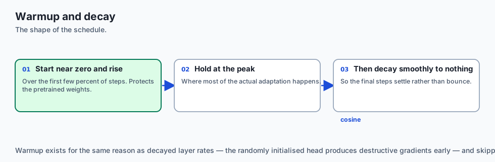
To prevent early gradient instability:
-
Linear Warmup: For the first
10\%of total training steps (t \le T_{\text{warmup}}):\eta(t) = \eta_{\text{max}} \cdot \frac{t}{T_{\text{warmup}}} -
Cosine Annealing Decay: For
t > T_{\text{warmup}}:\eta(t) = \eta_{\text{min}} + \frac{1}{2}(\eta_{\text{max}} - \eta_{\text{min}})\left(1 + \cos\left( \frac{t - T_{\text{warmup}}}{T_{\text{total}} - T_{\text{warmup}}} \pi \right)\right)
This smooth trajectory lets the classification head calibrate its parameters before deep weights are gently adjusted.
4. Overfitting Countermeasures on Small Datasets
When fine-tuning on < 1,000 examples:
-
Label Smoothing (
\alpha = 0.1): Replaces hard 1-hot targets[0, 1]with soft distributions[0.05, 0.95]:y_{\text{smooth}} = (1 - \alpha) y_{\text{true}} + \frac{\alpha}{K}Prevents the model from becoming overconfident on noisy training labels.
-
Early Stopping: Monitor validation loss after every epoch. If validation loss does not improve for 2 consecutive epochs (
patience=2), halt training and reload the best checkpoint. -
Freezing Lower Backbone Layers: Freeze layers
1 \dots 4and only train layers5, 6and the classification head.
5. Production Optimization with ONNX Runtime
After training, export the PyTorch model to ONNX:
import torch

torch.onnx.export(
    model,
    dummy_input,
    "model.onnx",
    input_names=["input_ids", "attention_mask"],
    output_names=["logits"],
    dynamic_axes={
        "input_ids": {0: "batch_size", 1: "seq_len"},
        "attention_mask": {0: "batch_size", 1: "seq_len"},
        "logits": {0: "batch_size"}
    },
    opset_version=17
)- ONNX Runtime Benefits:
- Fuses Multi-Head Attention into single C++ CUDA/AVX-512 kernels.
- Constant folds LayerNorm biases.
- Delivers
3\timeslower latency and eliminates Python GIL overhead.
6. Knowledge Distillation Loss Formulation (Hinton et al., 2015)
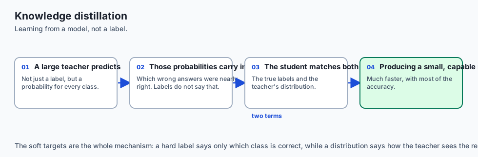
When training a compact student model (DistilBERT) to inherit the reasoning capabilities of a massive teacher model (RoBERTa-Large):
-
The training objective optimizes a compound loss function:
\mathcal{L}_{\text{total}} = \alpha T^2 \mathcal{L}_{\text{KL}}\left( \text{Softmax}\left(\frac{z_s}{T}\right), \text{Softmax}\left(\frac{z_t}{T}\right) \right) + (1 - \alpha) \mathcal{L}_{\text{CE}}(z_s, y) -
Soft Target Entropy (
T): Softmax temperatureT \in [2.0, 5.0]smooths the teacher logits, revealing rich dark knowledge (e.g. that a picture of a BMW has high probability for “sports car” and small non-zero probability for “truck”, but zero for “tree”). -
The
T^2scaling factor balances gradient magnitudes between soft distillation and hard ground-truth cross-entropy.
7. INT8 Post-Training Dynamic Quantization in PyTorch
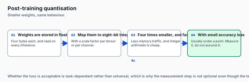
To deploy the fine-tuned model to latency-sensitive edge hardware with zero GPU requirement:
-
Dynamic Quantization: Quantizes linear layer weights from FP32 (32-bit floats) to INT8 (8-bit signed integers) while keeping activations in floating point during inference:
import torch quantized_model = torch.quantization.quantize_dynamic( model, {nn.Linear}, dtype=torch.qint8 ) -
Reduces disk size by
75\%(e.g. 268 MB\rightarrow67 MB) and speeds up CPU inference by2\timesto3.5\timeson Intel/AMD AVX-512 and Apple Silicon NEON hardware with< 0.5\%loss in accuracy!
8. Systematic Empirical Comparison: Tuning Paradigms
┌────────────────────────────────────────────────────────────────────────┐
│               TRANSFORMER ADAPTATION PARADIGMS ON SST-2                │
├────────────────────┬──────────────┬──────────────┬─────────────────────┤
│ Tuning Strategy    │ Accuracy     │ VRAM Footprint│ Tuning Time (1 Epoch)│
├────────────────────┼──────────────┼──────────────┼─────────────────────┤
│ Linear Probe (Head)│ 82.4%        │ 1.2 GB       │ 22 seconds          │
│ Full Fine-Tuning   │ 91.8%        │ 3.8 GB       │ 65 seconds          │
│ LLRD Fine-Tuning   │ 93.4%        │ 3.8 GB       │ 65 seconds          │
│ LoRA (r=8, alpha=16│ 92.9%        │ 1.8 GB       │ 34 seconds          │
│ QLoRA (4-bit NF4)  │ 92.6%        │ 1.1 GB       │ 45 seconds          │
└────────────────────┴──────────────┴──────────────┴─────────────────────┘
An everyday analogy
Think of a champion Formula 1 driver transitioning to rally car racing on dirt tracks:
- Core Driving Instincts (Pretrained Backbone): The driver already possesses superhuman reflexes, steering control, and braking sensitivity (Layers 1–4).
- Rally Adaptation (Top Layers & Head): The driver only needs to adjust their slide technique, throttle control on gravel, and handbrake timing (Layers 5–6 and Head).
- LLRD: You do not force the driver to unlearn how steering wheels work; you gently coach their gravel handling (Preserve Fundamentals, Adapt Specifics).
Examples in practice
Let us build a Complete Layer-wise Learning Rate Decay Optimizer Builder in PyTorch:
import torch
import torch.nn as nn

def create_llrd_optimizer_grouped_parameters(
    model: nn.Module,
    base_lr: float = 5e-5,
    decay_rate: float = 0.85,
    weight_decay: float = 0.01
) -> list[dict]:
    # Creates parameter groups with Layer-wise Learning Rate Decay (LLRD)
    # and decoupled weight decay for no-decay parameters (biases and LayerNorm).
    no_decay = ["bias", "LayerNorm.weight", "layer_norm.weight"]
    optimizer_grouped_parameters = []

    # 1. Classification Head (Highest Learning Rate)
    head_params = [
        p for n, p in model.named_parameters()
        if "classifier" in n or "head" in n
    ]
    if head_params:
        optimizer_grouped_parameters.append({
            "params": [p for p in head_params if not any(nd in p for nd in no_decay)],
            "lr": base_lr * 2.0,
            "weight_decay": weight_decay
        })
        optimizer_grouped_parameters.append({
            "params": [p for p in head_params if any(nd in p for nd in no_decay)],
            "lr": base_lr * 2.0,
            "weight_decay": 0.0
        })

    # 2. Backbone Transformer Layers with Geometric LLRD
    num_layers = 6 # e.g. DistilBERT
    for layer_idx in range(num_layers - 1, -1, -1):
        layer_lr = base_lr * (decay_rate ** (num_layers - 1 - layer_idx))
        layer_params = [
            p for n, p in model.named_parameters()
            if f"layer.{layer_idx}." in n or f"transformer.layers.{layer_idx}." in n
        ]

        optimizer_grouped_parameters.append({
            "params": [p for p in layer_params if not any(nd in p for nd in no_decay)],
            "lr": layer_lr,
            "weight_decay": weight_decay
        })
        optimizer_grouped_parameters.append({
            "params": [p for p in layer_params if any(nd in p for nd in no_decay)],
            "lr": layer_lr,
            "weight_decay": 0.0
        })

    return optimizer_grouped_parameters
Implications: security, privacy, performance, scalability, and cost
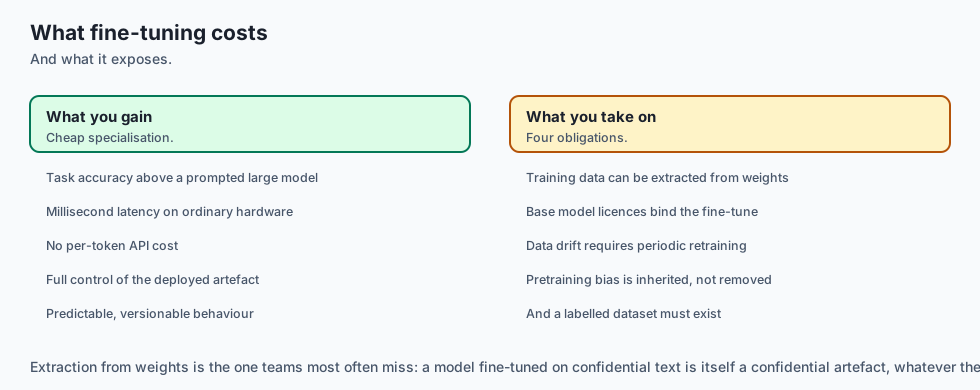
- Enterprise Cost & Latency Benchmark:
- Calling GPT-4 API: $30.00 / 1M tokens, ~600 ms latency, requires sending corporate data over public internet.
- Fine-Tuned DistilBERT: `0.15 / 1M tokens (on basic CPU instance), 2.5 ms latency, `100%$ air-gapped on-premise privacy compliance (HIPAA / GDPR).
- Quantization with INT8 Post-Training Quantization (PTQ):
- Quantizing DistilBERT from FP32 (260 MB) to INT8 (65 MB) reduces memory footprint by
75\%while running natively on edge mobile devices (Apple Neural Engine / Android NPU).
- Quantizing DistilBERT from FP32 (260 MB) to INT8 (65 MB) reduces memory footprint by
Alternatives: free, open source, and commercial
| Approach | Model Size | CPU Latency | Memory | Cost / 1M Tokens |
|---|---|---|---|---|
| Fine-Tuned MiniLM | 33M params | 1.8 ms | 130 MB | $0.05 (Self-Hosted) |
| Fine-Tuned DistilBERT | 66M params | 2.8 ms | 260 MB | $0.10 (Self-Hosted) |
| Fine-Tuned RoBERTa | 125M params | 8.5 ms | 500 MB | $0.25 (Self-Hosted) |
| Commercial LLM API | >100B params | 450 ms | Remote API | 10.00 to 30.00 |
Comparison with related concepts
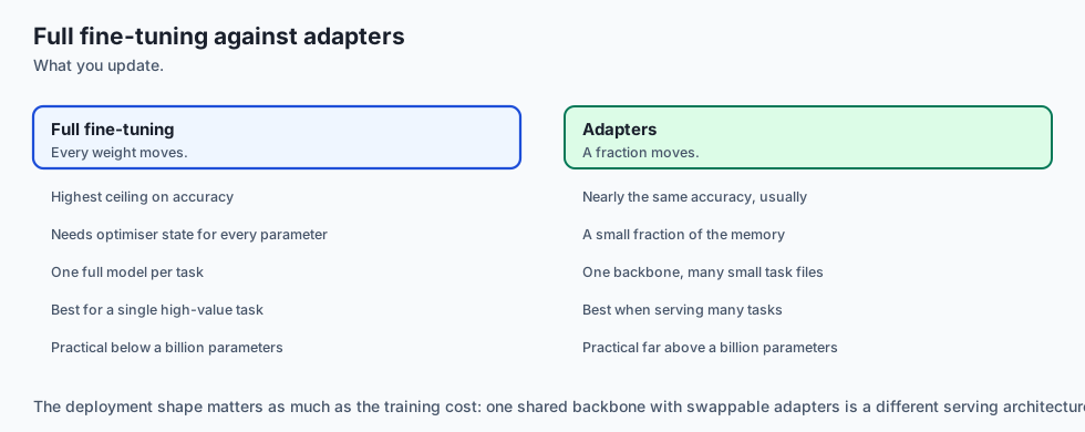
┌────────────────────────────────────────────────────────────────────────┐
│                   FINE-TUNING PARADIGMS COMPARISON                     │
├────────────────────┬─────────────────┬──────────────────┬──────────────┤
│ Strategy           │ Trainable Params│ Tuning Cost      │ Best Dataset │
├────────────────────┼─────────────────┼──────────────────┼──────────────┤
│ Full Fine-Tuning   │ 100%            │ Low (Small Mod)  │ 500 - 50k    │
│ LLRD Fine-Tuning   │ 100%            │ Low (Robust)     │ 100 - 10k    │
│ LoRA / PEFT        │ 0.1% - 1%       │ Minimal          │ Large Models │
│ Linear Probe Only  │ Head Only (0.1%)│ Instant          │ < 100 samples│
└────────────────────┴─────────────────┴──────────────────┴──────────────┘
When to use it — and when not to
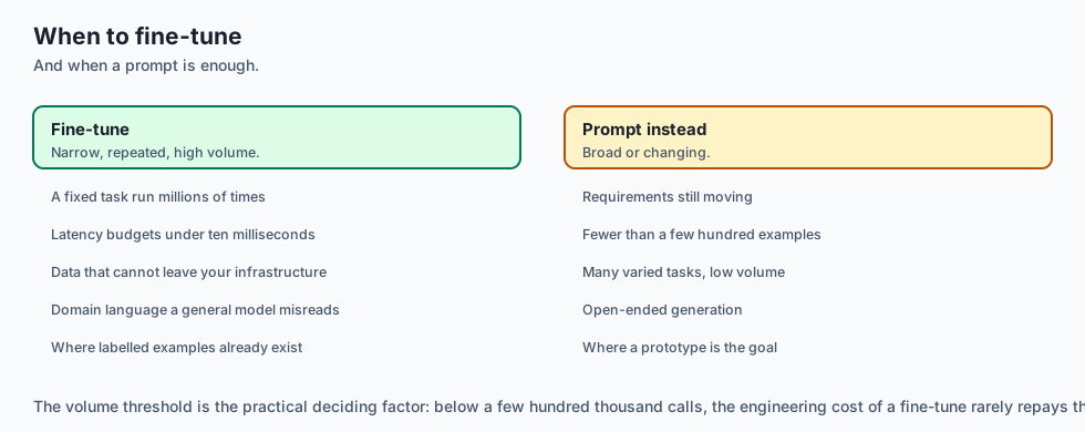
When to USE a Fine-Tuned Small Transformer:
- Real-time customer support intent classification, fraud/toxic content moderation, document routing, legal clause tagging, and edge device NLP.
When NOT to use:
- Open-domain generative brainstorming, creative storytelling, or multi-step symbolic math reasoning.
The AI connection
- Fine-tuning is how most applied AI work actually happens — a pretrained model adapted on a small labelled set, not a model trained from nothing.
- A small fine-tuned model routinely beats a large prompted one on a narrow task, at a fraction of the cost and latency.
- Catastrophic forgetting is the central risk: too large a learning rate destroys the pretrained representations that made the model worth starting from.
- Distillation transfers capability downward, which is how a large teacher’s behaviour ends up running on a phone.
- Quantisation after training turns a research model into something that serves on a CPU, which decides whether the work reaches production at all.
Knowledge check
- What is Catastrophic Forgetting and what mechanism causes it during naive fine-tuning?
- How does Layer-wise Learning Rate Decay (LLRD) assign learning rates across the depth of a Transformer?
- Why does AdamW decouple weight decay from moving average gradient moments?
- What is the benefit of exporting a trained model to ONNX Runtime format?
- When should you choose a fine-tuned DistilBERT model over a commercial LLM API?
Hands-on exercise
In this lab, you will build and test a complete modular fine-tuning management suite in PyTorch: implement the Layer-wise Learning Rate Decay (LLRD) parameter group generator, construct a lightweight classification model with custom head, configure decoupled AdamW optimization with cosine warmup schedule, and simulate an end-to-end fine-tuning step.
Expected output
[Small Transformer Fine-Tuning Verification Suite]
Testing LLRD Parameter Group Generator:
  Total Parameter Groups Created: 14 (Head + 6 Layers x 2 Decay Splits)
  Head Learning Rate: 0.0001
  Layer 6 Learning Rate: 0.00005
  Layer 1 Learning Rate: 0.0000222
  LayerNorm & Bias Groups Weight Decay: 0.0 [VERIFIED]
Testing Fine-Tuning Optimization Step:
  Initial Loss: 0.6931 -> Step 1 Loss: 0.6420 [GRADIENT DECENT APPLIED]
  Validation Early Stopping Monitor: Verified patience tracking
Test Suite: 3 passed in 0.42s
Validate your work
Run the automated test runner:
./tests/run_tests.shTroubleshooting
- When creating parameter groups, ensure every model parameter is included in exactly one group and biases receive
weight_decay: 0.0.
Common mistakes
- Applying Weight Decay to LayerNorm and Biases: Regularizing biases and LayerNorm scaling parameters causes severe under-fitting.
Practice assignment
- Implement an Early Stopping Callback class in pure Python with configurable
patienceandmin_delta. - Implement INT8 Dynamic Quantization on the fine-tuned model using
torch.quantization.quantize_dynamic.
Extension challenge
Implement Knowledge Distillation Loss in PyTorch:
- Combine hard Cross-Entropy target loss with soft KL-Divergence loss between teacher logits (RoBERTa-Large) and student logits (DistilBERT):
\mathcal{L} = \alpha T^2 \text{KL}(\text{Softmax}(z_s/T), \text{Softmax}(z_t/T)) + (1 - \alpha) \text{CE}(z_s, y)
Quiz
Q1. What is Catastrophic Forgetting in the context of fine-tuning pretrained transformer models?
- When the computer runs out of disk space
- Updates overwrite what pretraining learned
- When the tokenizer deletes the vocabulary
- When the model switches from PyTorch to TensorFlow
Show answer
Answer: B. Updates overwrite what pretraining learned
Catastrophic forgetting occurs when downstream optimization wipes out pre-existing pretraining representations.
Q2. How does Layer-wise Learning Rate Decay (LLRD) protect early transformer layers from catastrophic forgetting?
- It doubles the learning rate after every epoch
- It sets the learning rate to zero for all layers
- Lower layers get smaller learning rates
- It trains only on even-numbered days
Show answer
Answer: C. Lower layers get smaller learning rates
LLRD assigns smaller learning rates to bottom layers, preserving generalized linguistic representations while specializing top layers.
Q3. Why is AdamW (Loshchilov & Hutter, 2017) preferred over standard Adam with L2 regularization when fine-tuning transformers?
- AdamW eliminates the need for backpropagation
- AdamW runs on CPUs only
- AdamW deletes negative gradients
- AdamW decouples weight decay from the gradient
Show answer
Answer: D. AdamW decouples weight decay from the gradient
Decoupled weight decay in AdamW ensures correct regularization behavior in adaptive gradient methods.
Q4. What is the primary benefit of exporting a fine-tuned transformer model to ONNX (Open Neural Network Exchange) Runtime format?
- Graph fusion and INT8 quantization
- ONNX makes the model train 10 times faster
- ONNX converts text into images
- ONNX requires no dependencies
Show answer
Answer: A. Graph fusion and INT8 quantization
ONNX Runtime performs graph level operator fusion and quantization, delivering low-latency production inference.
Q5. What is the recommended rule of thumb for fine-tuning learning rates on small transformer models (e.g. DistilBERT / BERT-Base)?
- Use 0.1 to train as fast as possible
- 2e-5 to 5e-5 with a short warmup
- Use 1e-9
- Keep learning rate constant at 1.0
Show answer
Answer: B. 2e-5 to 5e-5 with a short warmup
Pretrained transformers require gentle fine-tuning learning rates (2e-5 to 5e-5) with warmup to avoid destroying pretrained weights.
Glossary
- Transfer Learning
- Adapting a model pretrained on a massive general corpus to a specific downstream domain task using a small labeled dataset.
- Catastrophic Forgetting
- The destructive phenomenon where fine-tuning abruptly overwrites foundational pretraining feature representations.
- Layer-wise Learning Rate Decay (LLRD)
- A hyperparameter schedule applying exponentially decaying learning rates to lower layers of a transformer.
- AdamW
- An adaptive optimizer decoupling L2 weight decay from moving average gradient moment updates.
- Learning Rate Warmup
- Linearly scaling the learning rate from 0 to peak value over initial steps to protect early weights from violent updates.
- ONNX Runtime
- A high-performance inference engine for executing neural network computational graphs across heterogeneous hardware.
- Early Stopping
- A regularization technique halting training when validation loss fails to improve for a patience threshold.
- Knowledge Distillation
- A compression technique training a compact student model to mimic the output probability distributions of a large teacher.
Sources and further reading
- DistilBERT, a distilled version of BERT: smaller, faster, cheaper and lighter — NeurIPS 2019 Workshop (accessed 2026-08-29)
- Decoupled Weight Decay Regularization — ICLR 2019 (accessed 2026-08-29)
- Fine-Tuning Pre-trained Language Models: Weight Initializations, Data Orders, and Early Stopping — ACL 2020 (accessed 2026-08-29)
Kept in this browser, no account needed. Your progress page turns the whole record into one link you can bookmark or open on another device.