Math, Statistics, and Data › Linear Algebra II and Calculus › Day 111
Day 111: Gradient Descent from Scratch
After this lesson you will know why the single line x <- x - eta * grad(x) is the whole of how every model in this course gets trained, and you will know it because you watched it fail first. You will run gradient descent on the simplest convex function there is, f(x) = 0.5*x^2, with a learning rate only slightly too large, and watch the loss climb on every step -- smoothly, plausibly, for thousands of iterations -- until it overflows to inf and the very next update becomes nan. Nothing will be wrong with the function, the gradient, or the code. Then you will derive, by hand, the exact regime structure that explains it: for f(x) = 0.5*a*x^2 the update is exact algebra, x_n = x_0*(1-eta*a)^n, and four learning rates on the same quadratic land in four different outcomes with EXACT boundaries at 1/a and 2/a -- monotone decrease, an exact landing on the minimum in one step, alternating-but-converging, and unbounded divergence. You will measure the per-step contraction ratio and watch it equal |1-eta*a| to float precision. You will meet conditioning: on a bowl with eigenvalues 1 and kappa, the optimal fixed learning rate is 2/(1+kappa), an isotropic bowl solves in exactly one step, and an ill-conditioned one needs more than ten times the steps -- Day 106's eigenvalues, shown to govern how hard optimisation actually is. You will add momentum, a running average of the gradient substituted for the raw gradient, and measure it beating plain descent at the identical learning rate on the same ill-conditioned bowl. You will build a gradient checker from Day 108's central difference and watch it catch a sign error in one component of a deliberately broken gradient and nothing else. You will run two initialisations on a non-convex function and watch them converge to two different minima, decided entirely by where they started. And you will catch a stopping-criterion trap in the act: a naive "the loss stopped changing" rule firing early on a genuinely convex, genuinely unsolved problem, while the gradient itself sits ten times above its own tolerance. Every number in this lesson comes from a script you can run yourself.
Hands-on lab for this lesson
Lab files on GitHub: https://github.com/ai-roadmap-365/ai-roadmap-365.github.io/tree/main/labs/sections/math-statistics-and-data/day-111-gradient-descent-from-scratch
- Get the hands-on files. Clone the labs repository once (you can reuse this clone for every lesson). This works on macOS, Linux, and Windows (PowerShell or WSL):
git clone https://github.com/ai-roadmap-365/ai-roadmap-365.github.io.git cd ai-roadmap-365.github.io - Open this lesson's lab. Move into the directory for this specific day. Every lab lives at the same predictable path — section / subsection / week / day:
cd labs/sections/math-statistics-and-data/day-111-gradient-descent-from-scratch - Read the lab guide. Open `README.md` in that directory. It lists the exact commands, what each does, the expected output, and how to check your work — read it before running anything.
- Run it and check your work. Follow the README's "How to run" section: run the example first to see the finished result, then complete the numbered exercises in `starter/`, then run the tests. The tests pass (exit 0) only when your work is correct.
bash tests/run_tests.sh # or the test command named in the lab README
You can also open the lab as a local page (works offline, shows the file tree and expected output).
Learning objectives
By the end of this lesson you will be able to:
- State the entire gradient-descent update rule from memory, x <- x - eta*grad(x), and explain each of its four parts: the current point, the gradient, the scaled step, and the new point
- Derive the closed-form solution of gradient descent on a 1-D quadratic, x_n = x_0*(1-eta*a)^n, and use it to predict the exact learning-rate boundaries 1/a and 2/a
- Classify a learning rate into one of four regimes -- monotone, exact, oscillating-but-converging, divergent -- from first principles, and verify the classification against a real run
- Explain why the gradient points uphill and why the update subtracts rather than adds it
- Connect an ill-conditioned Hessian (Day 106's ratio of eigenvalues) to slow convergence under a fixed learning rate, and state the optimal fixed learning rate for a quadratic bowl
- Implement momentum as an exponentially weighted running average of the gradient, and explain why it helps on an ill-conditioned problem in terms of averaging away an oscillating component
- Implement a numerical gradient check using Day 108's central difference and use it to localise a bug to a specific parameter
- State three common stopping criteria for gradient descent and explain a concrete case where a loss-based criterion fails while a gradient-based one does not
- Explain, from a captured run, what a diverging training run looks like numerically -- a smoothly increasing loss, then inf, then nan -- and why production training loops check their own loss for finiteness
- Compare hand-rolled gradient descent against scipy.optimize.minimize, torch.optim.SGD and jax.grad with optax, stating when each is the right choice and which of them were actually run in this lesson
- Explain why non-convex loss landscapes make initialisation a real decision rather than an implementation detail
Prerequisites
- Day 108 -- derivatives, the central difference, and the U-shaped error curve. The gradient check in this lesson is that same central difference, used to catch bugs rather than just to measure derivatives
- Day 109 -- partial derivatives and the gradient. Today's update rule subtracts exactly that vector
- Day 110 -- the chain rule and backpropagation. Day 110 computes gradients; today uses them. Neither day is the other
- Day 106 -- eigenvalues and eigenvectors. The condition number governing today's ill-conditioning section is literally the ratio of two eigenvalues of a Hessian
- Day 43 -- python3 -m venv and installing a package with pip
- Days 71-74 -- pytest, which the lab uses for both the reference suite and the running score
- Comfort writing a Python function that takes another function as an argument
Why this matters
Here is a function with one variable, one minimum, and nothing subtle about it: f(x) = 0.5 * x². Its derivative is x. Its minimum is at x = 0. A first-year calculus student solves it by inspection. There is no reason this should ever go wrong.
Run gradient descent on it anyway, starting at x = 1, with a learning rate of 2.2. Watch the loss.
step |     x            | loss
   0 |  1.0000000000 | 0.5000000000
   1 | -1.2000000000 | 0.7200000000
   2 |  1.4400000000 | 1.0368000000
   3 | -1.7280000000 | 1.4929920000
   4 |  2.0736000000 | 2.1499084800
   5 | -2.4883200000 | 3.0958682112
   6 |  2.9859840000 | 4.4580502241
   7 | -3.5831808000 | 6.4195923227
   8 |  4.2998169600 | 9.2442129448
   9 | -5.1597803520 | 13.3116666404
  10 |  6.1917364224 | 19.1687999622
  11 | -7.4300837069 | 27.6030719456
  ...
The loss is going up. Every single step. Not because the function changed, not because the gradient is wrong, not because of a bug anywhere in the code. Run it further — the real run in this lesson’s lab went to 4,000 steps — and the value keeps growing, alternating sign, doubling and redoubling, until at step 3890 it exceeds the largest number a float64 can represent and becomes inf. The very next update subtracts one infinite quantity from another and produces nan. From that point on, every number in the run is garbage, and nothing raised an exception to tell you.
The function was never the problem. The gradient was never the problem. The problem was one number: the learning rate, η, which decided how far to move at every step. 2.2 is not a wild, obviously-broken value — it is 0.2 past the function’s own boundary of 2.0. A learning rate you might type without a second thought, on the simplest convex function that exists, turns a solved problem into a training run that silently destroys itself.
That is today’s subject, and it is the reason the phrase “just call .fit()” hides more than it should. Every model trained in the remaining 250-plus days of this course — every linear regression, every neural network, every large language model — is trained by some variant of one loop:
x ← x − η · ∇f(x)Day 109 gave you ∇f(x), the gradient: the direction that increases f fastest. Day 110 gave you the machinery — the chain rule, backpropagation — for computing that gradient efficiently through an arbitrarily deep composition of operations. Today you take the step. You will discover that the entire mechanics of training a model, stripped of every optimiser, every scheduler and every trick this course reaches later, is a single line of arithmetic — and that almost everything that goes wrong in practical training traces back to how carefully that one line’s single free parameter, η, was chosen.
By the end of this lesson you will have derived, by hand, the exact boundaries at which a learning rate stops working — not approximate, not “usually around here”, but exact fractions computable from the curvature of the function you are minimising. You will have measured why some loss landscapes are intrinsically harder to descend than others, connected directly to the eigenvalues you met on Day 106. You will have built the single most useful debugging technique in this entire subject — checking a gradient against a number that has never heard of your formula — and watched it catch a real bug. And you will understand, precisely, why “the loss stopped changing” is not the same claim as “we are done”.
The idea in plain language
You are standing on a hillside in thick fog. You cannot see the valley floor, but you can feel which way the ground slopes under your feet. The rule for getting down is not complicated: feel which way is steepest uphill, turn around, and take a step. Then do it again. And again.
That sentence is gradient descent, completely. ∇f(x) is “which way is steepest uphill, from here.” The minus sign is “turn around.” η is “how big a step.” Repeating the whole thing is “and do it again.”
Two things about walking downhill in fog are worth sitting with, because they are exactly the two things that make the mathematics of this lesson necessary rather than decorative.
The size of your step matters enormously, and the slope alone does not tell you what size to pick. A cautious two-inch shuffle will get you down eventually, correctly, but it could take until nightfall on a gentle slope. A confident three-metre stride is efficient on that same gentle slope — and, on a steep-sided gully, sends you flying past the bottom and up the opposite wall, possibly higher than where you started. The same step size is wise in one place and reckless in another, and the terrain is exactly what decides which.
You only ever know the slope where you are standing. You cannot see the whole valley from the fog. Each step is a local decision, made with local information, and the accumulated sequence of those local decisions either walks you steadily to the bottom or walks you somewhere else entirely — off a cliff, in circles, or to a false bottom that is not the true lowest point of the whole landscape.
That second observation is where a plain hillside analogy runs out and the mathematics has to start doing real work. On an actual hillside, “steepest” and “true bottom” are things your eyes and feet can often just tell you. A loss surface with a hundred million dimensions offers no such luxury — the only thing you get to know at any point is the local gradient, computed exactly (thanks to Day 110), and the only decision you get to make is how far to step along it. Today is about that one decision, examined so carefully that its exact failure boundaries fall out of pure algebra.
Historical background
The method of following the gradient downhill by fixed steps is old — the core idea traces to work by the French mathematician Augustin-Louis Cauchy in 1847, describing what is now called the method of steepest descent for solving systems of equations. Cauchy’s version was not aimed at anything resembling machine learning; it was a numerical technique for a mathematics that predates computers by a century.
The method sat as one numerical-optimisation tool among several for a long time. Its rehabilitation as the central algorithm of a major branch of computing came from a specific, later development: the practical trainability of artificial neural networks once backpropagation (Day 110) made it computationally cheap to obtain the gradient of a scalar loss with respect to every parameter in a large model at once. Once that gradient became affordable, the question of what to do with it — a question gradient descent had already answered in the nineteenth century — became urgent again.
Two refinements matter enough to name here, both revisited properly later in this course. Stochastic gradient descent, where the gradient is estimated from a small random batch of data rather than computed exactly over an entire dataset, made training on datasets too large to fit the exact-gradient computation in memory not just feasible but standard. Momentum, the technique this lesson’s lab builds from scratch in exercise 6, was described by Boris Polyak in 1964 as a way of accelerating the classical method on ill-conditioned problems, well before it became a default ingredient of neural-network training.
What is worth taking from the history rather than any particular date: this is not a technique invented for AI and later found to be useful elsewhere. It is a general numerical-optimisation idea, older than the electronic computer, that turned out to be exactly the tool an entirely different field needed a century later, once that field acquired a way to compute the one ingredient the method requires — the gradient — cheaply enough to use it hundreds of thousands of times per training run.
What it is — and what it is not
Gradient descent is: an iterative method for finding a point where a differentiable function is small, by repeatedly moving from the current point in the direction opposite to the gradient, scaled by a learning rate.
| The belief | What is actually true |
|---|---|
| ”Gradient descent finds the minimum” | It finds a point where the gradient is (near) zero. On a convex function that is the global minimum. On the non-convex functions this course spends most of its time on, it is one of possibly many local minima, and which one you reach depends on where you started — exercise 8 in the lab demonstrates this with two starting points and two different answers. |
| ”A smaller learning rate is always safer” | Safer against divergence, yes. But this lesson’s own regime table shows a smaller η inside the safe range converges more slowly, not more safely in any useful sense — you traded a real risk (divergence) for a real cost (wasted compute), and the trade is not free. |
| ”The loss going down means it is working” | The loss can go down for a while even with a wrong gradient (a partially-correct direction still often has positive dot product with the true one) or right up until the moment a run diverges, as the opening example shows for the first twenty steps. Loss decreasing is necessary but not remotely sufficient evidence that everything is correct. |
| ”Gradient descent and backpropagation are the same thing” | No — and Day 110 already made this point once, worth restating with today’s context added. Backpropagation computes the gradient. Gradient descent uses it. You can compute a gradient and do something else with it entirely (sensitivity analysis, for instance), and you can obtain a gradient some other way and still run gradient descent with it. |
| ”Momentum, Adam and other optimisers are unrelated to plain gradient descent” | They are gradient descent with the raw gradient in the update rule replaced by something derived from it — a running average, an adaptively-scaled version, and so on. Exercise 6 in the lab builds the simplest possible case, momentum, and the update rule is still recognisably x ← x − η·(something built from the gradient). |
Why it was created and what problems it solves
The problem: you have a function of possibly millions of variables, you can evaluate it and its gradient, and you need a point where it is small — without any closed-form way to solve ∇f(x) = 0 directly.
For the simplest functions, calculus gives you an exact answer: set the derivative to zero and solve algebraically. Day 111’s own running example, f(x) = 0.5·a·x², has derivative a·x, and a·x = 0 is solved instantly by x = 0. You did not need gradient descent for that — and the lesson uses it anyway, deliberately, because a problem simple enough to solve exactly is also simple enough to let you verify every claim about the iterative method by comparing it against the known right answer.
Real problems in this course do not offer that luxury. A loss function defined by a neural network with a hundred million parameters has no algebraic solution to ∇f(x) = 0 that anyone can write down. What you do have, thanks to Day 110, is a cheap way to compute ∇f(x) at any specific point x — one backward pass, costing about as much as the forward pass that produced the loss in the first place. Gradient descent is the answer to the question: given that you can only ever evaluate the gradient at one point at a time, how do you turn a sequence of such evaluations into a point where the function is small?
The answer’s entire content is contained in one line, and the rest of this lesson is about making that one line trustworthy:
x ← x − η · ∇f(x)The gradient supplies the direction. Nothing else in the algorithm supplies direction — it is the only directional information the method ever uses. Everything else the algorithm needs to decide — how far to move, when to stop, what to do about a landscape with more than one valley — is a separate decision layered on top of that one piece of information, and each of those decisions is a section of this lesson.
How it works
The update rule, taken apart
Four quantities, in order:
x_n           the current point
∇f(x_n)       the gradient at that point -- computed exactly, via Day 110
−η · ∇f(x_n)  the ACTUAL step: flip the gradient's direction, scale its length by η
x_n+1 = x_n + step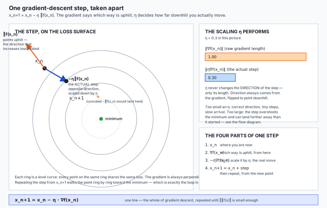
Two roles are easy to conflate and worth separating cleanly. The gradient’s direction always points uphill — that is its definition, unrelated to anything about training. The learning rate’s only job is to scale the length of the step that direction gets flipped into. η never changes which way you move, only how far. Get the direction wrong (a sign error, a stale value) and no learning rate fixes it. Get the length wrong and the direction was never the issue.
The one function this whole lesson is built on
Everything from here forward uses one deliberately simple function:
f(x) = 0.5 · a · x² f'(x) = a · xIts derivative is linear in x, which means the gradient-descent update is exact algebra, not an approximation:
x_(n+1) = x_n − η · (a · x_n) = x_n · (1 − η·a)Every step multiplies x by the same fixed number, (1 − η·a). That means after n steps:
x_n = x_0 · (1 − η·a)^nThis closed form is the whole lesson in one line. Whether the sequence x_n shrinks to zero, lands on zero, oscillates while shrinking, or explodes depends entirely on the magnitude of (1 − η·a) — and that magnitude is something you can compute in advance, exactly, from η and a alone.
The four regimes, derived and then measured
Write c = 1 − η·a, the contraction factor. |c| decides everything:
Condition on η (with a = 5, so 1/a = 0.2, 2/a = 0.4) | Value of c | What happens |
|---|---|---|
0 < η < 1/a | 0 < c < 1 | x shrinks toward 0 every step, same sign throughout — monotone |
η = 1/a | c = 0 | x becomes exactly 0 after one step — exact |
1/a < η < 2/a | −1 < c < 0 | x flips sign every step, but ` |
η = 2/a | c = −1 | x flips sign every step and ` |
η > 2/a | c < −1 | ` |
This table is not a rule of thumb. It is the complete case analysis of |c|^n as n → ∞, and every boundary in it — 1/a and 2/a — is an exact fraction, not an estimate.
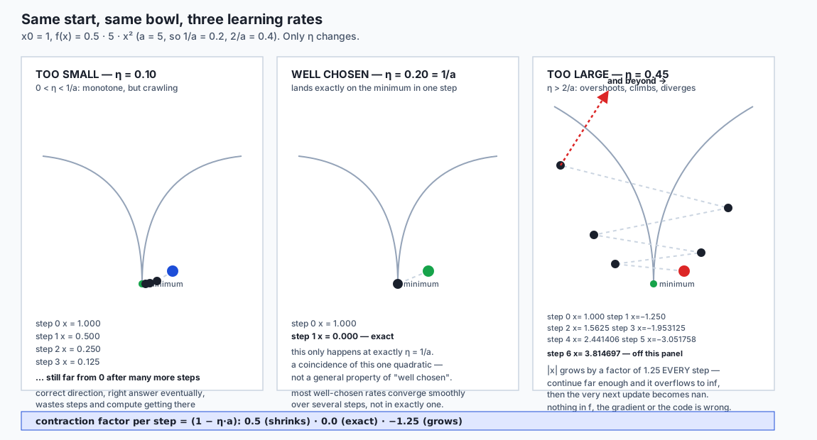
A real run confirms all four rows, with a = 5:
η | Regime | First four steps | Classified as |
|---|---|---|---|
0.10 | 0 < η < 1/a | 1.0, 0.5, 0.25, 0.125 | monotone |
0.20 | η = 1/a | 1.0, 0.0, 0.0, 0.0 | exact |
0.35 | 1/a < η < 2/a | 1.0, -0.75, 0.5625, -0.4219 | oscillating |
0.45 | η > 2/a | 1.0, -1.25, 1.5625, -1.9531 | divergent |
Those four rows came from lab/examples/02_regimes_and_contraction.py, and the lab’s classify_regime function derives the label purely from the observed values in each run — never by reading η and a and looking the answer up. That distinction matters: a classification function that just re-derives the table above from the inputs would be checking that the table was typed correctly, not that the algorithm actually behaves the way the table claims.
The contraction factor, measured directly
The closed form predicts that the ratio |x_(n+1) / x_n| should equal |c| = |1 − η·a| at every single step, not just on average. This is checkable, and the lab checks it:
| η | Predicted |1 − η·a| | Measured ratio (first three steps) | Match |
| --- | --- | --- | --- |
| 0.10 | 0.500000 | 0.5, 0.5, 0.5 | to 1e-9 |
| 0.35 | 0.750000 | 0.75, 0.75, 0.75 | to 1e-9 |
| 0.45 | 1.250000 | 1.25, 1.25, 1.25 | to 1e-9 |
The three measured ratios are constant across steps and match the prediction to float precision — not “roughly”, to 1e-9, because this is exact multiplication in floating point and the only source of disagreement possible is rounding, which for a handful of steps is many orders of magnitude smaller than the tolerance. This is exactly the kind of prediction Day 108 taught you to distrust until you have measured it, and here it survives the measurement completely.
Conditioning: when the landscape itself is the problem
Everything above used one variable. Real loss landscapes have millions. The moment you have more than one dimension, a new failure mode appears that no single learning rate can fully escape: the landscape can be steep in one direction and shallow in another, at the same point.
Take the two-variable bowl:
f(x, y) = 0.5 · (x² + κ·y²)Its Hessian — the matrix of second derivatives Day 106 introduced — is diag(1, κ), a diagonal matrix whose two eigenvalues are 1 and κ. The condition number of this bowl is κ, exactly: the ratio of its largest eigenvalue to its smallest, which Day 106 defined as the quantity that governs how “well-behaved” a matrix is. Here it governs something very concrete: how hard this particular landscape is to descend.
There is a standard, provably-optimal fixed learning rate for a quadratic bowl with smallest eigenvalue μ and largest eigenvalue L:
η* = 2 / (μ + L)For this bowl, μ = 1 and L = κ, so η* = 2/(1+κ). At κ = 1 (an isotropic bowl — equally steep in every direction) that optimal rate is η* = 1, and — this is not a coincidence, it is the two-dimensional version of the “exact” row in the regime table above — gradient descent with the optimal rate solves an isotropic quadratic bowl in exactly one step.
As κ grows, the optimal rate 2/(1+κ) shrinks, because it has to stay small enough to avoid divergence along the steep direction (whose own eigenvalue is κ). But the shallow direction (eigenvalue 1) never got any steeper — it is being forced to creep forward using a learning rate sized for a completely different, much steeper problem. That is the entire mechanism of ill-conditioning, stated without a single approximation.
Measured, on the same bowl, at its own optimal learning rate, for four condition numbers:
κ | Optimal η = 2/(1+κ) | Steps to ‖∇f‖ < 1e-4 |
|---|---|---|
| 1 | 1.000000 | 1 |
| 5 | 0.333333 | 27 |
| 20 | 0.095238 | 122 |
| 100 | 0.019802 | 691 |
Non-decreasing at every step up in κ, and κ = 100 needs 691 steps against κ = 1’s single step — more than a hundred times more, comfortably clearing “at least ten times” with room to spare. Nothing about η was mistuned in any of these four runs; each one used the provably optimal fixed learning rate for its own problem. The slowdown is not a tuning failure. It is what a large ratio between eigenvalues costs you, and no fixed learning rate — optimal or otherwise — escapes it. This is where Week 16’s two halves meet: Day 106 gave you eigenvalues as an abstract property of a matrix; today, the ratio of two of them is directly, measurably, the reason one optimisation problem needs six hundred times more steps than another that looks superficially similar.
Momentum: the minimal fix for zig-zag
The ill-conditioning table above used the best fixed learning rate available and still paid a steep price. Momentum is the smallest change that helps without abandoning the one-line update rule:
v ← β·v + ∇f(x)          (a running average of recent gradients)
x ← x − η·v               (step using the average, not the raw gradient)
This is not a new algorithm bolted onto gradient descent — it is the same update rule, x ← x − η·(something), with the raw gradient replaced by an exponentially weighted running average of it. β (a number between 0 and 1) controls how much of the past is remembered; β = 0 recovers plain gradient descent exactly, since v then equals the current gradient at every step.
Why does averaging help on the ill-conditioned bowl specifically? Along the steep direction, gradient descent overshoots and the gradient flips sign step after step — a genuinely oscillating signal, and an average of a signal that keeps flipping sign partially cancels itself. Along the shallow direction, the gradient keeps the same sign step after step, so an average of a consistently-signed signal does not cancel — it accumulates, and v grows larger than any single gradient in that direction ever was. The net effect is exactly what the ill-conditioned bowl needed: damping where the raw gradient was overreacting, reinforcement where it was crawling.
Measured, on the κ = 20 bowl, giving momentum the identical learning rate plain descent used:
| Method | η (identical for both) | Steps to ‖∇f‖ < 1e-4 |
|---|---|---|
| Plain gradient descent | 0.095238 | 122 |
Momentum (β = 0.5) | 0.095238 | 34 |
A 3.6× reduction in steps, from changing nothing but what stands in for the gradient in an otherwise identical update rule. Do not read this as “momentum is magic” — it is averaging, doing exactly what averaging does to an oscillating signal versus a consistent one, on a problem specifically shaped to make that distinction pay off.
Gradient checking: catching a bug that will not announce itself
Day 108 built the central difference — (f(x+h) − f(x−h)) / (2h) — as a way to measure a derivative numerically. Today it earns its keep a second time, as a way to check one you derived analytically.
The failure mode gradient checking exists to catch is specific and dangerous: an analytic gradient with a bug that produces numbers of a plausible type, plausible shape and plausible magnitude — and is simply wrong. Such a bug does not crash. It does not always even stop training from working, because a partially-wrong direction can still have positive dot product with the true gradient and make the loss go down for a while. The only reliable way to catch it is to compare against something that shares none of its assumptions: a numerical estimate that knows nothing about how the analytic formula was derived.
Take a three-parameter function, f(x,y,z) = x² + 2y² + 0.5z³, whose correct gradient is (2x, 4y, 1.5z²). Deliberately flip the sign of the middle component, and check both against a central difference component by component, at (0.7, -1.3, 2.1):
| Component | Correct gradient check | Buggy gradient (sign flipped on y) check |
|---|---|---|
x | pass | pass |
y | pass | fail |
z | pass | pass |
The correct gradient passes on every component. The buggy one fails on exactly the one that was broken and nowhere else — because the check compares each component of the analytic gradient against its own independent numerical estimate, with no interaction between components. This is the single most useful debugging technique in the whole of practical machine-learning mathematics, and it costs almost nothing to run once per new gradient you write by hand.
Non-convexity: where you start is part of the answer
Every function used so far has had one minimum. Take f(x) = (x² − 1)² instead: it has minima at x = −1 and x = +1 (both with value 0), and a local maximum at x = 0 sitting between them, since f'(x) = 4x³ − 4x is negative for 0 < x < 1 (pulling toward +1) and positive for −1 < x < 0 (pulling toward −1).
Run gradient descent from two starting points, one on each side of the maximum:
| Start | Converged to |
|---|---|
x₀ = −0.1 | −1.000000 |
x₀ = +0.1 | +1.000000 |
Two runs, same algorithm, same learning rate, same number of steps — different answers, separated by 2.0, comfortably past any reasonable margin for “these are genuinely different minima.” The only thing that differed between the two runs is which side of x = 0 they started on. On a non-convex loss surface — which is what every neural network in this course trains on — initialisation is not an implementation detail you can be careless about. It is part of what determines the answer you get.
The stopping-criterion trap
Every gradient-descent loop needs a rule for when to stop. Three are common:
| Criterion | What it checks | What can go wrong |
|---|---|---|
‖∇f(x)‖ < tol_grad | Is the gradient small? | The most honest of the three — directly checks the thing that defines a minimum — but can be expensive to evaluate exactly on very large models |
| ` | Δf | < tol_f` |
| A maximum iteration count | Have you run out of patience? | Catches nothing about whether training actually succeeded; only prevents running forever |
The middle row is the trap, and it is worth seeing it actually spring rather than taking the warning on faith. Take a genuinely convex bowl with a very small curvature, f(x) = 0.5 · 0.0001 · x², starting far from its minimum at x = 100:
gradient at x=100:   0.01      (10x above a tolerance of 0.001)
one step later, delta_f:   1.0e-07   (below a tolerance of 0.000001)
The gradient is comfortably above its own tolerance — this point is nowhere near converged. The change in loss from a single step, though, is smaller than its tolerance, because the curvature is so small that even a real, non-trivial gradient produces a barely-perceptible change in the function’s value. A naive |Δf| < tol_f rule stops here. A ‖∇f‖ < tol_grad rule correctly refuses to. “The loss stopped changing” is not the same claim as “we converged”, and this is not a contrived edge case — it is exactly the shape of a long, gently sloped approach to a minimum, which real loss landscapes have plenty of.
An everyday analogy
Return to the fogbound hillside, and let it carry every piece of today’s mathematics through to the end.
The gradient is the slope under your feet, right now. It tells you nothing about the rest of the mountain — only which way is steepest, from exactly where you are standing, this instant.
The learning rate is your stride length. A tiny, cautious stride is always safe — it will never send you flying past the bottom — but on a gentle slope it is needlessly slow, the monotone regime’s whole story. A stride tuned exactly to the local steepness can, in the fortunate case of a perfectly uniform slope, land you at the bottom in one confident step — the exact regime. Push your stride a little further and you overshoot the bottom and land partway up the opposite wall, but each overshoot is smaller than the last, so you still arrive, just zig-zagging — the oscillating regime. Push it further still and each overshoot lands you higher on the opposite wall than where you started, and you climb, alternately, out of the valley entirely — divergence, and the opening failure of this lesson exactly.
A narrow, steep-walled gully is the ill-conditioned bowl. A stride safe for its steep walls is comically small relative to how gently the gully’s floor actually slopes lengthwise, so you take tiny, safe side-to-side corrections while making almost no progress along the gully’s length. A wide, gently-sloped bowl — walls and floor equally steep — is the well-conditioned case, where one confident stride, correctly sized, gets you most of the way there.
Momentum is remembering which way you have been generally heading. If your last several steps have zig-zagged left-right-left-right across the gully, that side-to-side motion averages toward nothing, and you can safely discount it. If your last several steps have all trended the same direction along the gully’s length, that trend is real, and leaning into it — walking a bit further than any single step’s slope alone would suggest — is exactly the right thing to do.
Gradient checking is asking a second, independent guide to point. If your reading of the slope under your feet and a companion’s independent reading disagree sharply in one specific direction, you trust the disagreement, not either reading alone — and you find out which direction they disagree about, rather than distrusting the whole hike.
Non-convexity is a mountain range with more than one valley. Which valley you end up in is decided by which slope you started walking down, not by anything about your stride length or your patience once you are already descending. Two hikers starting a few metres apart, on opposite sides of a ridge, can end their walk kilometres apart, in different valleys, having done everything else identically.
The stopping-criterion trap is mistaking a long, gentle, boring stretch of trail for having arrived. If you only check “did the ground under me change much in the last minute,” a long, flat-feeling stretch that is still genuinely sloping downhill — just very gradually — will read as “we must be there,” when the honest check is not how the trail felt, but whether the ground is actually level yet.
Examples in practice
The full arithmetic behind the opening failure
a = 1, η = 2.2. The divergence boundary is 2/a = 2.0, and η sits 0.2 past it. The contraction factor is c = 1 − 2.2 = −1.2, so |c| = 1.2 > 1: this is the divergent regime, and x_n = x_0 · (−1.2)^n.
Since f(x) = 0.5·x², the loss at step n is 0.5 · (1.2)^(2n) = 0.5 · 1.44^n. Each step multiplies the loss by 1.44 — a genuine, if modest-looking, 44% increase per step. Modest per step, but compounding: after 20 steps the loss has grown by 1.44^20 ≈ 511, and by step 3890 the tracked value has passed 8.6 × 10^307 — one step short of float64’s largest representable number, ~1.8 × 10^308. Step 3891 pushes it over, to inf, and the arithmetic of the next update (inf − η·inf, which involves subtracting two infinite quantities whose relative sizes floating point can no longer resolve) produces nan.
Every number in that paragraph came from lab/examples/01_the_hook.py, run for real, not derived and hoped for.
The full arithmetic behind the two-minima result
f(x) = (x²−1)², f'(x) = 4x³ − 4x = 4x(x²−1) = 4x(x−1)(x+1). The three roots of the derivative — x = −1, 0, 1 — are exactly the two minima and the one local maximum. Starting at x₀ = 0.1, comfortably inside (0, 1), f'(0.1) = 4(0.1)(0.01 − 1) = 4(0.1)(−0.99) = −0.396: the gradient is negative, so x ← x − η·(−0.396) = x + η·0.396 moves x in the positive direction — toward +1, away from the maximum at 0. By symmetry, starting at x₀ = −0.1 moves toward −1. Two runs of 400 steps each, at η = 0.05, land at −0.9999999999999999 and 0.9999999999999999 respectively — both within 1e-3 of the algebraically exact answer, and 1.9999999999999998 apart, well past this lesson’s 1.5 margin for “these are genuinely different.”
Implications: security, privacy, performance, scalability, and cost
Performance and cost. The learning rate is the single hyperparameter most directly responsible for whether a training run’s compute budget is well spent or wasted. A learning rate inside the safe range but too small (this lesson’s monotone regime) wastes steps — and every wasted step on a large model is real GPU-hours billed by the hour. A learning rate past the divergence boundary does not merely waste compute; it destroys the run entirely, and the run’s true cost includes however many steps passed before anyone noticed the loss had actually been nan for the last several hours.
Scalability. Ill-conditioning gets worse, not better, as models grow. A larger model has more parameters, which generally means a Hessian with a wider spread between its smallest and largest eigenvalues — a larger condition number, in exactly the sense this lesson measured. This is a direct, mechanical reason (not a hand-wave) that naive fixed-learning-rate gradient descent scales poorly, and it is the practical motivation for every adaptive-learning-rate method this course reaches later: they are, at their core, attempts to give different directions in a high-dimensional space something closer to their own appropriately-sized learning rate, rather than forcing one global η to serve every direction at once.
Numerical robustness. The opening failure is not a special case reserved for badly-chosen toy examples. Overflow to inf followed by nan is exactly what a diverging training run looks like on real hardware, and neither event raises an exception by default in IEEE-754 arithmetic. A training loop that does not explicitly check its own loss for finiteness after every step will happily continue computing — and billing — with nan parameters for as long as it is left running. This is one of the cheapest, highest-value guards a training script can contain, and today’s opening failure is the exact mechanism it exists to catch.
Security. A silently wrong gradient — caught by the checking technique in this lesson, uncaught otherwise — produces a model that trains, has plausible-looking loss curves, and learns something incorrect in a way that is not obvious from the training logs alone. In any setting where a trained model’s decisions have consequences for people, “the loss went down” is not evidence the model learned the right thing, and gradient checking is one of the few genuinely cheap ways to rule out an entire, dangerous class of silent bug before it ever reaches a real training run.
Privacy. Not the direct subject of today’s lesson, but worth stating plainly since it follows immediately from the update rule: every step of gradient descent uses a gradient computed from specific training examples. A gradient is not an anonymous summary of the data that produced it — this is the entire basis of gradient-inversion attacks in the federated-learning literature, where an adversary who observes only the gradients (never the raw data) can sometimes reconstruct the data those gradients came from. The mathematics you built today is the same mathematics whose output, in an adversarial setting, is a data-leakage surface.
Alternatives: free, open source, and commercial
Four ways to run gradient descent, from the one built entirely by hand today to the tools that run it at production scale. Only the hand-rolled NumPy and pure-Python versions in this lesson’s lab were actually run here. SciPy, PyTorch and JAX are not installed in this authoring environment, and no output from any of them is reproduced anywhere in this lesson or its lab — everything said about them below is drawn from their own documentation and marked as such.
| Tool | What it does | Exact or approximate? | Cost |
|---|---|---|---|
| Hand-rolled NumPy / pure Python (this lab) | The update rule, written out explicitly, on scalar and small-vector problems | Exact arithmetic on the quadratics used here | Free — the standard library plus NumPy |
scipy.optimize.minimize | A general-purpose scalar-function minimiser with several selectable algorithms | Exact gradients if you supply them; numerically estimated otherwise | Free, open source (BSD) |
torch.optim.SGD | Gradient descent (with optional momentum, weight decay, Nesterov acceleration) as one step of a PyTorch training loop, driven by autograd-computed gradients | Exact gradients via automatic differentiation | Free, open source; commercial only via the compute you run it on |
jax.grad with optax | Functional gradient transformation (jax.grad(f) returns a new function computing f’s gradient) paired with a library of optimiser update rules, including SGD and momentum variants | Exact gradients via automatic differentiation | Free, open source |
The engine you built here. Choose it when the goal is understanding the mechanics themselves, or when you are debugging a training run and need to reason about why an optimiser behaves the way it does rather than treating it as a black box. Its concrete example is every script in this lesson’s lab — the whole update rule, all nine exercises, in well under two hundred lines. Its limitation is entirely engineering: no automatic differentiation (Day 110’s engine supplies gradients on real models), no GPU dispatch, no batching. Nothing about the idea changes when those are added.
scipy.optimize.minimize — according to its documentation, it exposes a single function with a method parameter selecting among several classical optimisation algorithms ('BFGS', 'CG', 'Nelder-Mead', among others), accepts an optional analytic gradient via the jac argument and falls back to a numerical estimate if none is given, and returns a result object carrying the optimum, the function value there, and convergence diagnostics. Choose it for classical numerical-optimisation problems with a modest number of variables — fitting a small model, solving an inverse problem — where you want a well-tested general-purpose solver rather than to write the loop yourself. It is not the tool of choice for training a neural network with millions of parameters; the algorithms it offers are generally not designed for that scale or for stochastic (mini-batch) gradients.
torch.optim.SGD — according to its documentation, it is constructed with an iterable of parameters to optimise, a required lr argument, and optional momentum, dampening, weight_decay and nesterov arguments, and its .step() method applies one update to every tracked parameter using whatever gradient PyTorch’s autograd most recently computed for it (via .backward()). Choose it as the default first optimiser for a PyTorch training loop; its momentum argument is a direct production implementation of exactly the mechanism exercise 6 builds by hand in this lesson’s lab, down to the same v ← β·v + ∇f shape.
jax.grad with optax — according to its documentation, jax.grad(f) is a function transformation: given a function f, it returns a new function that computes f’s gradient, rather than a value computed once. optax then supplies composable optimiser update rules — optax.sgd(learning_rate, momentum=...) among them — designed to be combined with JAX’s functional style and its jit compilation. Choose this combination when you want gradient computation and optimiser logic to compose as ordinary function transformations, or when targeting JAX’s compiled-and-accelerated execution model specifically.
The honest summary: for understanding what gradient descent actually does, write it yourself once, as this lab does. For running it at any scale that matters, the production tools exist precisely because the engineering — automatic differentiation over arbitrary computation graphs, batching, hardware dispatch — is substantial, well-solved, and not worth re-deriving. The update rule itself, underneath all four rows of that table, is the same line this lesson opened with.
Comparison with related concepts
Gradient descent and backpropagation (Day 110). Different jobs, constantly confused. Backpropagation computes ∇f(x). Gradient descent uses it to update x. You could compute a gradient with backpropagation and never run gradient descent at all — sensitivity analysis is exactly that. You could run gradient descent with a gradient obtained some other way (finite differences, for a small enough problem) and never touch backpropagation.
Gradient descent and Newton’s method. Both are iterative optimisation methods that use derivative information. Newton’s method also uses the second derivative (the Hessian) to choose both the direction and an effectively per-direction step size, which is why it can solve a quadratic bowl in one step regardless of its condition number — unlike gradient descent, whose one-step-solves-it property in this lesson was special to the isotropic case. That extra power costs a Hessian, which for a model with millions of parameters is far too large to compute or store; gradient descent’s appeal is precisely that it needs only the (comparatively cheap) gradient.
The learning rate and other hyperparameters. The learning rate is a hyperparameter — a value that controls the training process rather than one the training process learns. It sits alongside the momentum coefficient β from exercise 6, the batch size, and the network architecture itself: none of these are updated by gradient descent’s own update rule, even though gradient descent is what tunes everything that is a parameter.
Convex and non-convex optimisation. A convex function has exactly one basin, so any local minimum gradient descent finds is automatically the global one — this lesson’s quadratic and ill-conditioned bowl are both convex. A non-convex function, like exercise 8’s two-minima example, can have multiple basins, and gradient descent finds whichever one it happened to be walking downhill into. Almost every model trained in this course, beyond the earliest and simplest, has a non-convex loss surface.
Stopping criteria and convergence proofs. A convergence proof (which this lesson has effectively supplied, in closed form, for the 1-D quadratic case) tells you the algorithm reaches the minimum in the mathematical limit. A stopping criterion is the separate, practical decision about when to actually stop a finite-length run and call the current point good enough — and, as the plateau example showed, a badly chosen stopping criterion can declare victory well before the mathematics behind the convergence proof has actually delivered it.
When to use it — and when not to
Use plain gradient descent whenever you have a differentiable objective and a cheap way to compute its gradient, and the objective is convex or you have accepted that you will find a local minimum rather than provably the global one. It is the correct starting point for almost every training loop in this course.
Use a smaller learning rate than you think you need when you are uncertain about a landscape’s curvature and have not measured its condition number. The cost of too-small an η is wasted steps, which is expensive but recoverable. The cost of too-large an η is the opening failure of this lesson, which is not recoverable without restarting.
Use momentum, or a more sophisticated optimiser built on the same principle, whenever you suspect (or, better, have measured, as this lesson’s lab does) that your loss surface is ill-conditioned — which for realistic neural-network loss surfaces is close to the default assumption rather than a special case.
Use gradient checking the first time you write any gradient by hand, and every time you change how one is computed. It is cheap, mechanical, and catches exactly the class of bug — plausible-looking, partially-correct, silently wrong — that no amount of watching the loss curve will reliably reveal.
Do not trust a single fixed learning rate across wildly different phases of a long training run. The condition number of a real loss surface is not necessarily constant as training progresses; a rate that was well-chosen early on can become poorly chosen later, which is the practical motivation for learning-rate schedules this course covers separately.
Do not use a loss-based stopping criterion alone on any landscape you have not specifically confirmed lacks the kind of plateau this lesson demonstrated. Prefer a gradient-norm-based criterion, or combine both with a maximum-iteration ceiling as a backstop rather than a primary decision rule.
Do not assume a non-convex training run’s result is initialisation-independent without testing more than one initialisation. Exercise 8’s two-minima function is a toy, deliberately small enough to solve by hand — but the mechanism it demonstrates, that where you start can determine which answer you get, is exactly as real on a loss surface with a hundred million dimensions.
Knowledge check
Eight questions accompany this lesson, covering: the exact regime boundaries 1/a and 2/a and what happens past each; why the update rule subtracts rather than adds the gradient; how the measured contraction ratio predicts convergence speed quantitatively; how a Hessian’s condition number governs the cost of ill-conditioning and why the optimal fixed learning rate cannot fully escape it; the mechanism by which momentum’s averaging helps an oscillating-versus-consistent gradient signal differently; what a component-wise gradient check actually catches and why it localises a bug rather than merely detecting one; the concrete case where a loss-based stopping criterion disagrees with a gradient-based one; and what a diverging run actually looks like, measured, before it destroys itself.
Two are worth attempting before reading anything else: the one asking what a learning rate just past 2/a produces, and the one asking why “the loss stopped changing” is not the same claim as “we converged.” Those two facts are the load-bearing ones this entire lesson is built to demonstrate rather than merely assert.
Hands-on exercise
The lab is “Descent by Hand”, and its centrepiece is the training loop itself, x ← x − η·∇f(x), built from nothing and pushed until it breaks.
cd labs/sections/math-statistics-and-data/day-111-gradient-descent-from-scratch
python3 -m venv .venv
.venv/bin/pip install -r requirements/requirements.txt
Nine exercises, in order, in starter/descent.py, working against constants and helper functions already written out for you in starter/dataset.py. Check yourself as you go:
.venv/bin/pytest starter -qUnattempted work is reported as skipped, never as failed. Wrong work fails with your answer printed beside the correct one.
Expected output
An untouched checkout:
1 passed, 20 skippedA finished one, every test passing. The full harness ends with:
50 checks, 0 failure(s).and exits 0. Along the way, the opening failure, captured from a real run:
step 0 |  1.0000000000 | loss 0.5000000000
step 1 | -1.2000000000 | loss 0.7200000000
  ...
x first becomes inf at step 3890
x first becomes nan at step 3891
and the ill-conditioning result the whole day is built on:
kappa |     eta = 2/(1+kappa)  | steps
    1 |               1.000000 | 1
    5 |               0.333333 | 27
   20 |               0.095238 | 122
  100 |               0.019802 | 691
Validate your work
bash tests/run_tests.sh; echo "exit=$?"prints50 checks, 0 failure(s).andexit=0..venv/bin/pytest examples -q -p no:cacheproviderprints24 passed..venv/bin/pytest starter -q -p no:cacheproviderprints1 passed, 20 skippedon an untouched checkout, and every test passing when you are finished.- Each of the four reference scripts ends with
every assertion held. - Your
classify_regimeagrees with the four rows in this lesson’s regime table on all four of the exactηvalues used throughout — not approximately, exactly, since the underlying arithmetic is exact.
Troubleshooting
ModuleNotFoundError on dataset or descent means you ran a reference script from the lab directory rather than from inside examples/; they import their neighbours from beside themselves.
Tests that keep skipping after you have written code usually mean a leftover return None survived below your implementation — every skeleton in starter/descent.py has it on the last line of a docstring.
A classify_regime that reports “divergent” for a run that is actually converging usually means your shrinking check has no tolerance for float rounding on the very last step; the reference implementation allows 1e-12 of slack for exactly this reason.
A contraction ratio that does not match |1 − η·a| on the “exact” regime (η = 0.2) is expected to fail if you have not excluded the step where x_n = 0 — dividing by zero there is not a bug in your formula, it is a genuine division by zero that per_step_ratios must skip.
troubleshooting.md covers all of these in full, along with the momentum update-order mistake, the two-minima run that collapses onto one basin, and why the harness clears bytecode caches at the start of its run.
Common mistakes
- Trusting a “safe-looking” learning rate without checking
2/a.2.2looks like an ordinary number. It is0.2past the exact boundary fora = 1. - Assuming a smaller learning rate is free of cost. It only trades divergence risk for wasted compute; both are real costs, on opposite ends of the same knob.
- Tuning one learning rate for an ill-conditioned problem and expecting it to be fast. The optimal fixed rate for
κ = 100still needs691steps. No single fixedηescapes ill-conditioning; only a change to the update rule itself (momentum, or the adaptive methods this course reaches later) does. - Trusting a decreasing loss curve as proof of a correct gradient. A partially-wrong gradient can still decrease the loss for a while. Check the gradient itself, component by component, against an independent numerical estimate.
- Stopping on
|Δf| < tolalone. It can fire on a plateau that is nowhere near a minimum. Prefer‖∇f‖ < tol, or use both together.
Practice assignment
Extend the lab and put a prediction to a real measurement, the way every section of this lesson did.
- Find your own divergence boundary. Pick a value of
aother than1or5, predict the exact boundary2/a, and confirm with a real run thatηjust below it converges (however slowly) whileηjust above it diverges. - Predict a step count before measuring it. Using the condition-number table’s four rows, fit (by eye, or with a simple regression) how steps-to-tolerance scales with
κ, then predict the step count forκ = 500before running it, and compare. - Sweep the momentum coefficient. Run momentum at
βvalues other than0.5on theκ = 20bowl, and find the value ofβ(to one decimal place) that needs the fewest steps in your own measurements. Report both the count and the value. - Write your own gradient-checking failure. Construct a second buggy gradient — not a sign flip this time, but a coefficient error (a
2xwritten as3x, for instance) — and confirmgradient_checkstill catches it at the lab’s tolerance. - Build a second plateau. Using a different curvature and starting point than the lab’s, construct another case where
|Δf| < tol_ffires while‖∇f‖remains above its own tolerance, and report both numbers.
Extension challenge
Three, in increasing order of difficulty.
Push the ill-conditioning table further, and predict before you measure. The lab’s table stops at κ = 100. Extend it to κ = 1000 and κ = 10000, predict the step counts from the pattern in the existing four rows before running anything, then measure and report how good your prediction was.
Derive the momentum stability boundary. This lesson stated momentum’s update rule without deriving its own divergence boundary, the way section “The four regimes” derived plain gradient descent’s. Work out, for the 1-D quadratic f(x) = 0.5·a·x², the condition on η, a and β under which momentum’s update converges rather than diverges, and confirm it numerically by finding a (η, β) pair your formula predicts should diverge and watching it do so.
Implement Nesterov’s variant and explain why it helps. Look up Nesterov accelerated gradient — the variant of momentum where the gradient is evaluated at the look-ahead point x − η·β·v rather than at the current x — and implement it as a fourth function in your own copy of the lab. Compare its step count against plain momentum’s on the κ = 20 bowl, and write one paragraph on why evaluating the gradient at the look-ahead point, rather than the current point, is expected to help.
The AI thread. This loop, unchanged in shape, trains every model the rest of this course builds — linear models, small networks, and eventually architectures with more parameters than anyone could list by hand. Nothing about the update rule gets more sophisticated as models grow; x ← x − η · ∇f(x) is exactly as true for a hundred-billion-parameter language model as it is for the single-variable quadratic this lesson opened with. What changes with scale is everything around the rule — how the gradient is computed (Day 110’s machinery, applied to an unimaginably larger graph), how much data one step sees, whether the learning rate is fixed or scheduled or adapted per-parameter — but the core arithmetic never leaves this lesson’s one line.
The learning rate is the hyperparameter most directly responsible for whether a training run works at all, and you have now seen exactly why, in closed form, on a function simple enough to check every claim by hand. When a large training run’s loss suddenly spikes to nan after appearing to train normally for hours, the mechanism is not usually mysterious — it is very often a learning rate that was fine for the loss surface’s condition early in training and stopped being fine later, producing exactly the smoothly-increasing-then-overflowing pattern this lesson opened with, just on a landscape too large to inspect by eye. You now know what that failure looks like from the inside, and — for the one-dimensional case, exactly — precisely where its boundary sits.
Quiz
Q1. For f(x) = 0.5*a*x^2 with a = 5, gradient descent uses a learning rate of eta = 0.45. What happens, and why?
- It diverges, because eta = 0.45 is above the boundary 2/a = 0.4
- It converges monotonically, because 0.45 is a small number
- It lands exactly on the minimum in one step, because 0.45 is close to 1/a
- It oscillates forever without ever converging or diverging, because eta is between 1/a and 2/a
Show answer
Answer: A. It diverges, because eta = 0.45 is above the boundary 2/a = 0.4
The update is exact algebra: x_n = x_0*(1 - eta*a)^n. At eta = 0.45 and a = 5, (1 - eta*a) = 1 - 2.25 = -1.25, whose absolute value exceeds 1 -- so |x| grows by a factor of 1.25 every single step, without bound. The boundaries are exact: 0 < eta < 1/a = 0.2 gives monotone decrease, eta = 0.2 lands exactly on zero in one step, 0.2 < eta < 2/a = 0.4 gives alternating-but-shrinking convergence, and eta > 0.4 diverges. 0.45 sits past that last boundary. The lab measures this directly rather than trusting the formula: gradient_descent(lambda x: 5*x, 1.0, 0.45, 30) grows the tracked value past 800 within 30 steps.
Q2. Gradient descent subtracts the gradient rather than adding it. Why?
- It is an arbitrary convention that could equally well have been addition
- The gradient points in the direction of steepest ASCENT, so subtracting it moves toward lower loss
- Addition would make the learning rate negative, which is not allowed
- Subtraction is computationally cheaper than addition in floating point
Show answer
Answer: B. The gradient points in the direction of steepest ASCENT, so subtracting it moves toward lower loss
The gradient is defined as the direction of steepest increase (Day 109). To reduce loss you need to move in the OPPOSITE direction, which is exactly what subtracting the gradient does: x <- x - eta*grad(x). This is not a convention or an efficiency choice -- it is the one direction, among all directions from a point, that decreases the function fastest, and subtracting the gradient is how you take it. Adding the gradient would be gradient ASCENT, which is a real and useful algorithm for a different goal: maximising a function rather than minimising one.
Q3. Two learning rates are tried on the same 1-D quadratic: eta1 gives a measured per-step ratio |x_(n+1)/x_n| of 0.9, and eta2 gives a measured ratio of 0.3. Which converges faster, and how much faster, after 20 steps?
- They converge at the same rate, because both ratios are below 1
- It cannot be determined without knowing a and eta individually
- eta2, by a factor of about (0.3/0.9)^20, which is an enormous number
- eta1, because a ratio closer to 1 means steadier progress
Show answer
Answer: C. eta2, by a factor of about (0.3/0.9)^20, which is an enormous number
The ratio |1 - eta*a| IS the per-step contraction factor, so after n steps the remaining distance to the minimum is multiplied by ratio^n. After 20 steps, eta1 leaves 0.9^20 = 0.12 of the original distance, while eta2 leaves 0.3^20 = 3.5e-11 of it -- eta2's remaining error is smaller by a factor of roughly 3.5e9. A ratio closer to 1 means SLOWER shrinkage, not steadier progress; ratio = 0 (the exact regime) is the fastest possible. This is exactly what exercise 4 measures: the ratio predicted from eta and a matches the ratio measured from a real run to float precision.
Q4. A bowl f(x, y) = 0.5*(x^2 + kappa*y^2) is used to study ill-conditioning. At the optimal fixed learning rate 2/(1+kappa), what happens as kappa grows from 1 to 100?
- The problem becomes unsolvable once kappa exceeds 2, since the learning rate formula would be undefined
- The number of steps shrinks, because a larger kappa makes the bowl steeper overall and therefore faster to descend
- Nothing changes, because the optimal learning rate always converges in one step regardless of kappa
- The number of steps to reach a fixed gradient tolerance grows, because kappa = 1 solves in exactly one step while kappa = 100 needs far more
Show answer
Answer: D. The number of steps to reach a fixed gradient tolerance grows, because kappa = 1 solves in exactly one step while kappa = 100 needs far more
At kappa = 1 the bowl is isotropic (both eigenvalues equal 1), and the optimal learning rate 2/(1+1) = 1 solves it in exactly one step -- the 2-D analogue of the 1-D "exact" regime. As kappa grows, the optimal learning rate 2/(1+kappa) shrinks to stay stable on the steep direction, which then forces the shallow direction (whose own curvature never changed) to crawl. The lab measures 1, 27, 122 and 691 steps for kappa = 1, 5, 20 and 100 respectively -- strictly increasing, and kappa = 100 needs more than ten times kappa = 1's count. This is Day 106's condition number, made concrete: a large ratio between a Hessian's eigenvalues makes optimisation intrinsically harder, no matter how well you tune a single fixed learning rate.
Q5. Momentum replaces the raw gradient with v <- beta*v + grad(x) in the update x <- x - eta*v. On an ill-conditioned bowl, why does this help?
- Momentum increases the effective learning rate uniformly in every direction
- Momentum removes the need to choose a learning rate at all
- Averaging cancels an oscillating component of the gradient while a consistent component survives and accumulates
- Momentum replaces gradient descent with a fundamentally different, more powerful algorithm
Show answer
Answer: C. Averaging cancels an oscillating component of the gradient while a consistent component survives and accumulates
On the steep axis of an ill-conditioned bowl, the raw gradient overshoots and flips sign step after step -- an oscillating signal that a running average partially cancels, because opposite-signed contributions partly cancel each other in the average. On the shallow axis, the gradient keeps the same sign step after step -- a consistent signal that a running average does NOT cancel, so its contribution to v accumulates. The net effect is damped movement on the steep axis and reinforced movement on the shallow one, which is exactly the trade-off ill-conditioning punishes plain descent for. The lab measures it directly: at the identical learning rate plain descent uses on the kappa = 20 bowl, momentum with beta = 0.5 needs 34 steps against plain descent's 122. It is still the same update rule, x <- x - eta*(something); only what stands in for the gradient has changed.
Q6. A gradient-checking function is given an analytic gradient with the sign flipped on exactly one of three components. What should happen, and why is this check worth running?
- The check should report exactly the one broken component as wrong, because it compares each component of the analytic gradient against Day 108's central difference independently
- The check cannot detect a sign error, only a magnitude error
- The check is unnecessary if the loss still decreases during training
- The check should report all three components as wrong, because one wrong component corrupts the whole vector
Show answer
Answer: A. The check should report exactly the one broken component as wrong, because it compares each component of the analytic gradient against Day 108's central difference independently
Gradient checking compares the analytic gradient against a central difference COMPONENT BY COMPONENT, so a sign error in one component shows up as a disagreement in exactly that component and nowhere else -- the lab's test asserts the flags come back [True, False, True] for a three-component gradient with the middle sign flipped. The check is worth running precisely because "the loss still decreases" is not reliable evidence of a correct gradient: a wrong gradient that is only PARTLY wrong still has some correlation with the true one, so training can appear to work for a while even with a real bug present. Gradient checking is cheap, mechanical, and catches exactly the class of error that a decreasing loss curve cannot.
Q7. On a genuinely convex bowl, far from its minimum but with very small curvature, one gradient-descent step leaves the gradient at ten times its own tolerance while the change in loss falls below its own tolerance. What does this demonstrate?
- The function must actually be at a local minimum already, since the loss has stopped moving
- This can only happen on non-convex functions, never on a convex one
- The gradient tolerance and the loss tolerance must have been set inconsistently, since they disagree
- A stopping rule based only on the change in loss can fire before training has actually converged, while a gradient-norm-based rule correctly does not
Show answer
Answer: D. A stopping rule based only on the change in loss can fire before training has actually converged, while a gradient-norm-based rule correctly does not
This is a real, bounded convex bowl -- not a pathological edge case -- and one step from far away, with a small curvature, moves the loss by only a tiny amount even though the point is nowhere near its minimum and the gradient remains well above a reasonable tolerance. "The loss stopped changing" and "the gradient is near zero" are different claims, and this is the case where they disagree: the naive |delta f| < tolerance rule would stop here, wrongly, while the more honest ||gradient|| < tolerance rule correctly says training is not done. Nothing about convexity prevents this -- convexity guarantees a single global minimum exists, not that every approach to it changes the loss quickly.
Q8. A learning rate that is only slightly too large is used on the simplest convex function there is, f(x) = 0.5*x^2. What does the resulting run actually look like, measured?
- An immediate crash, since dividing by a number greater than 2/a raises an exception
- No visible difference from a correctly tuned run until the very last step
- A loss that oscillates between two fixed values forever, without ever growing or crashing
- A loss that increases every step, smoothly and plausibly, for thousands of iterations, before overflowing to inf and then nan on the very next update
Show answer
Answer: D. A loss that increases every step, smoothly and plausibly, for thousands of iterations, before overflowing to inf and then nan on the very next update
A measured run with eta = 2.2 (just above the divergence boundary 2/a = 2.0 for a = 1) shows the loss increasing on every one of its first 20 steps, and nothing about those early steps announces the coming failure -- the growth looks like an ordinary, if unwelcome, increasing curve. Continued for a few thousand more steps, the tracked value exceeds the largest representable float64 and becomes inf; the very next update then produces nan, since that step's arithmetic subtracts one infinite quantity from another. Neither transition raises an exception by default. This is exactly why production training loops check their own loss for finiteness: a run that "looks like it is training, just badly" can in fact be a diverging run that will eventually corrupt every parameter, and the earlier it is caught the cheaper the mistake.
Glossary
- Gradient descent
- The update rule x <- x - eta*grad(x), repeated until the gradient is small enough. Take the direction that increases loss fastest, flip it, scale it by a learning rate, and move. The entire training loop of every model in this course, underneath whatever else surrounds it.
- Learning rate
- The scalar eta that decides how far one gradient-descent step actually moves, written x <- x - eta*grad(x). It never changes the direction of the step, only its length. Too small wastes steps converging correctly; too large overshoots, and past a sharp boundary the run diverges outright.
- Contraction factor
- For a 1-D quadratic f(x) = 0.5*a*x^2, the number (1 - eta*a) that gradient descent multiplies x by on every step. Its absolute value predicts the whole outcome: below 1 the run shrinks toward the minimum, exactly 0 lands on it in one step, between 1 and 2 (in a*eta terms) it alternates sign while still shrinking, and above that it grows without bound.
- Divergence boundary
- The learning rate 2/a at which a 1-D quadratic gradient-descent run stops converging, even with alternating overshoot, and starts growing without bound. Above it, |x| grows by a fixed factor every step until the run overflows to inf and the next update becomes nan.
- Condition number
- The ratio of a Hessian's largest eigenvalue to its smallest (Day 106). For a bowl f(x,y) = 0.5*(x^2 + kappa*y^2), the condition number is kappa exactly. It governs how hard gradient descent's job is: a well-conditioned (low-kappa) bowl is fast to descend at any reasonable fixed learning rate, an ill-conditioned (high-kappa) one forces a tiny learning rate and therefore many more steps.
- Ill-conditioning
- A large gap between a loss surface's steepest and shallowest curvature directions. Any single fixed learning rate that is safe for the steep direction is forced to be small, which then makes progress in the shallow direction painfully slow -- the mechanism behind the textbook image of gradient descent zig-zagging down a narrow valley.
- Momentum
- An update that substitutes an exponentially weighted running average of the gradient, v <- beta*v + grad(x), for the raw gradient in the descent step: x <- x - eta*v. It is not a separate algorithm -- it is the same update rule with a smoothed direction, and it helps on an ill-conditioned bowl because averaging cancels an oscillating component while a consistent component survives.
- Gradient checking
- Comparing an analytic gradient function against Day 108's central difference, component by component, to catch implementation bugs. A wrong analytic gradient runs, returns numbers of a plausible shape, and can even make training loss go down for a while -- gradient checking is the cheap, mechanical way to catch it before it costs a real training run.
- Stopping criterion
- A rule that decides when to stop a gradient-descent loop: the gradient's norm falling below a tolerance, the change in loss between steps falling below a tolerance, or a maximum number of iterations. The first is the most honest; the second can fire early on a shallow, unsolved part of a landscape, mistaking a slow approach for arrival.
- Plateau
- A region of a loss surface where the function value changes very little from step to step even though the gradient has not vanished -- distinct from a true flat region where the gradient itself is near zero. A stopping rule that only watches the loss cannot tell the two apart, and can declare victory on a plateau that is nowhere near a minimum.
- Non-convex function
- A function with more than one local minimum (or a mix of minima, maxima and saddle points). Gradient descent on a non-convex function converges to whichever minimum is downhill from its starting point, so the initialisation is a real decision with a real effect on the answer, not an implementation detail.
- Overflow to inf, then nan
- What a diverging gradient-descent run looks like numerically in IEEE-754 floating point: the tracked value grows without bound until it exceeds the largest representable float and becomes inf, after which the next arithmetic operation (inf minus a finite multiple of inf, for instance) produces nan. Neither raises an exception by default -- a training loop must check its own loss for finiteness to catch this.
- Hyperparameter
- A value that controls how an algorithm runs rather than being learned by it -- the learning rate and momentum coefficient in this lesson are both hyperparameters. Unlike a model parameter, a hyperparameter is not updated by the gradient; it is chosen (or searched over) before or between training runs.
Sources and further reading
- Numerical Computation — Deep Learning (Goodfellow, Bengio, Courville) (accessed 2026-08-17)
- scipy.optimize.minimize — SciPy (accessed 2026-08-17)
- torch.optim.SGD — PyTorch (accessed 2026-08-17)
- jax.grad — JAX (accessed 2026-08-17)
- numpy.gradient — NumPy Developers (accessed 2026-08-17)
Kept in this browser, no account needed. Your progress page turns the whole record into one link you can bookmark or open on another device.