Math, Statistics, and Data › pandas and Data Wrangling › Day 125
Day 125: Cleaning Messy Data
After this lesson you will be able to name the exact statistic mean imputation cannot disturb (the mean) and the two it always does (the standard deviation, which strictly shrinks, and a real correlation, which strictly attenuates toward zero); explain algebraically why an imputed value can never inflate a correlation with an untouched column; distinguish fillna(0) from a genuine missing-value fill and name a case where zero collides with a value the data already contains; choose among dropna's how, thresh and subset arguments and state the row count each produces; show why ffill on unsorted data is a real bug and confirm sorting first fixes it; build a missing-indicator column that survives after isna() no longer can; count exactly how many values pd.to_numeric(errors='coerce') silently converted to missing; normalise string categories and show a raw groupby splitting one true category into several; distinguish exact duplicates from duplicates on a named subset and say which definition answers which question; and write a cleaning contract that asserts its own post-conditions and is proven able to raise.
Hands-on lab for this lesson
Lab files on GitHub: https://github.com/ai-roadmap-365/ai-roadmap-365.github.io/tree/main/labs/sections/math-statistics-and-data/day-125-cleaning-messy-data
- Get the hands-on files. Clone the labs repository once (you can reuse this clone for every lesson). This works on macOS, Linux, and Windows (PowerShell or WSL):
git clone https://github.com/ai-roadmap-365/ai-roadmap-365.github.io.git cd ai-roadmap-365.github.io - Open this lesson's lab. Move into the directory for this specific day. Every lab lives at the same predictable path — section / subsection / week / day:
cd labs/sections/math-statistics-and-data/day-125-cleaning-messy-data - Read the lab guide. Open `README.md` in that directory. It lists the exact commands, what each does, the expected output, and how to check your work — read it before running anything.
- Run it and check your work. Follow the README's "How to run" section: run the example first to see the finished result, then complete the numbered exercises in `starter/`, then run the tests. The tests pass (exit 0) only when your work is correct.
bash tests/run_tests.sh # or the test command named in the lab README
You can also open the lab as a local page (works offline, shows the file tree and expected output).
Learning objectives
By the end of this lesson you will be able to:
- State which statistic mean imputation cannot change (the mean) and which two it always does (standard deviation, which strictly shrinks, and correlation with an untouched column, which strictly attenuates)
- Explain, from the Pearson correlation formula, why an imputed value -- sitting exactly at the column mean -- can only dilute an existing correlation, never inflate one
- Distinguish fillna(0) from a true missing-value fill, and identify when 0 is itself a real, already-present value the fill would collide with
- Choose among dropna's how='any', how='all', thresh= and subset= arguments and predict the row count each produces on a given frame
- Demonstrate that ffill on unsorted data produces a wrong result at specific rows, and that sorting by the relevant column first produces the correct one
- Build a missing-indicator column recording isna() BEFORE imputing, and confirm it still matches the original mask after the fill has erased the evidence from the column itself
- Use pd.to_numeric(errors='coerce') and count exactly how many values were silently converted to missing, comparing that count against the number of unparseable values planted
- Normalise string categories with .str.strip(), .str.lower() and .str.replace(), and show nunique() and a raw groupby both revealing the damage of skipping that step
- Distinguish DataFrame.duplicated()'s exact-duplicate count from duplicated(subset=[...])'s subset-duplicate count, and state which definition answers which real question
- Detect outliers with the IQR rule or a z-score, and explain why detection is a statistical procedure while removal is a judgement call about whether the point is an error or a fact
- Write a cleaning contract asserting no nulls in key columns, declared dtypes, and a row count within an expected range, and prove it can genuinely raise on violating data
- Explain why imputing with a statistic computed over the whole dataset before a train/test split leaks information from the test set into training, and why SimpleImputer's fit/transform boundary exists specifically to prevent it
Prerequisites
- Days 120-124 -- pandas Series and DataFrames, loading and inspecting data, selecting and filtering, groupby and aggregation, and merging and reshaping. Not re-taught here.
- Day 116 -- the mean's zero breakdown point and robust measures of spread, which motivate why a single imputed statistic is not the whole picture
- Day 117 -- bias does not shrink with sample size, which is why informative (MNAR) missingness is not fixed by collecting more rows
- A working python3 on your PATH; the lab creates its own virtual environment with pandas 3.0.5 pinned exactly
Why this matters
Here is a cleaning step that looks like careful, responsible practice. Run it on pandas 3.0.5 and read the three numbers twice before moving on:
>>> income.mean()
52666.679...
>>> income.fillna(income.mean()).mean()
52666.679...
A column of customer income has ten missing values out of forty. You impute them with the column’s own mean — the standard textbook move, the one every “handling missing data” tutorial recommends first. You check the mean afterward, the way anyone would, to make sure nothing broke. It is identical to six decimal places. The imputation looks safe.
It is not safe, and the mean is exactly the wrong thing to have checked. Here is what actually moved, captured from the same real run:
income.std()  before imputation:  10663.947
income.std()  after  imputation:   9195.697   -- strictly smaller

corr(income, spending)  before:        0.745156
corr(income, spending)  after:         0.606148   -- strictly smaller in magnitude
The standard deviation dropped by nearly 14%. The correlation between
income and a genuinely related second column, spending, weakened by
almost a fifth of its own value. Nothing raised. Nothing warned.
fillna() ran, returned a DataFrame with no missing values, and quietly
changed the shape of the data in two ways you would only notice if you
had thought to check something other than the one number that could not
possibly have moved.
That last clause is the whole subject of this lesson, stated as bluntly as it deserves: the mean is guaranteed not to change under mean imputation, by construction — which means checking it proves nothing at all. Ten new points, each sitting exactly on the column’s own average, cannot pull the average anywhere. But they can shrink the spread around it, because “exactly average” is a very specific, very narrow thing to be ten times in a row. And here is the part worth sitting with, because it runs against the first intuition most people have: it is tempting to guess that ten points which “agree with the average” would somehow make income and spending look more related, not less — a pile of perfectly unremarkable points nodding along with everything. The measured direction is the opposite. An imputed value’s deviation from the mean is exactly zero, and in the arithmetic that defines a correlation, a zero deviation on one side of a pair can only ever contribute zero to the relationship between the two columns — it dilutes, it never strengthens. This lesson proves that claim from the arithmetic itself, not just from one dataset, later in How it works.
This is worth a direct note before you read any further, because it matters for how you should read the rest of this course: the working assumption behind Day 125, when it was first planned, was that mean imputation inflates correlations — “a pile of perfectly average points that agree with everything.” That assumption was tested directly against real code before this lesson was written, and it was wrong. Correlation attenuates. Every number in this lesson and its lab reflects the measured result, not the original guess, and that reversal is itself the lesson’s best illustration of its own argument: check what actually happened, not what a plausible story predicted would happen.
Days 120 through 124 built the machinery this lesson now has to use
carefully: dtypes and Copy-on-Write, the loading and inspection battery,
boolean masks and the partition invariant, split-apply-combine, and joins
with validate=. Every one of those days assumed the data, once loaded,
was worth trusting. This lesson is about the step in between — the one
where a genuinely messy dataset gets turned into something the rest of
this course’s tools can be pointed at safely, and where every single
decision made along the way (fill this, drop that, coerce this column,
collapse these three spellings into one) is a real, irreversible choice
about data you do not have. Day 126 turns today’s techniques into a
reproducible pipeline; today is about the techniques themselves, and what
each one actually costs.
The AI-practice stakes could not be more direct. Every cleaning decision
in this lesson changes the values a feature column ends up carrying into
training. Impute a missing income with the population mean before
splitting into train and test, and you have leaked the test set’s own
statistics into the imputation the training set relies on — the model
then scores better on evaluation than it has any right to, for reasons
nobody debugging it later will think to look for, because nothing failed
loudly. The arithmetic behind that leak is the exact arithmetic this
lesson opens with. By the end of today you should be unable to type
fillna() without immediately asking: what is this fill claiming about
the data I do not have, and what, specifically, will it change?
The idea in plain language
Cleaning feels like tidying. It is not. Every step in this lesson — filling a gap, dropping a row, coercing a string to a number, collapsing three spellings of “USA” into one, deciding an extreme value is an error rather than a fact — makes an irreversible decision about data that no longer exists to check against. You do not get to ask the missing income value what it actually was. You choose a number to stand in for it, and from that moment on, every downstream computation treats your choice as if it were the truth.
The habit this lesson tries to install is simple to state and hard to
practice: judge every cleaning step by what it changes, never by
whether it makes a warning go away. fillna() making .isna().sum()
report zero is not evidence of anything except that fillna() ran. The
question that actually matters is what moved — which statistics shifted,
which categories merged, which rows disappeared, and whether the shift is
one you can defend to someone who will use the cleaned data for something
you did not anticipate.
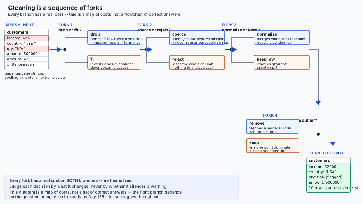
Look at the architecture diagram below. A messy DataFrame enters on the left, carrying missing values, garbage strings, inconsistent category spellings and a handful of extreme numbers. It does not pass through one cleaning step; it passes through a sequence of forks, each one a real decision with a name and a cost written on it: drop the row, or fill it — and if you fill it, with what? Coerce this column to a number, or reject the whole load? Normalise this string, or trust it as written? Remove this outlier, or keep it as a fact about the world? Every fork has two branches, and this lesson’s argument is that neither branch is free — the diagram is a map of costs, not a flowchart of “correct” answers.
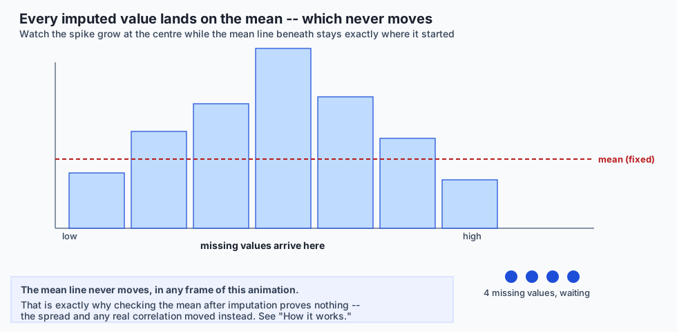
The animated diagram makes the opening failure concrete. Watch a distribution with a visible gap where its missing values sit. As imputation runs, each missing value arrives at exactly the same point — the column’s mean — and the histogram grows a spike exactly there, a spike that was never part of the original data. Below it, a single number, the mean itself, sits on a line that does not move at all through the entire animation. That is the whole argument in one picture: the number you would think to check is the one number the operation cannot touch.
The everyday analogy that carries the rest of this lesson: imagine a class attendance sheet with a few names missing from a given day, and a teacher’s aide who fills every blank with “average student” rather than leaving it blank or asking who was actually absent. The class roster now looks complete. Nobody notices anything wrong from the roster alone. But “average student” was never a real person, does not belong to any demographic group, does not have a real transcript, and — worst of all — “average student” appears on every single day some real student’s attendance would have told you something specific about that day. Every technique in this lesson is a variation on the same choice: invent an “average student,” leave the blank and lose that row, or go back and actually find out who was absent and why. Only the third option recovers the truth; the first two are both compromises, and knowing exactly what each one costs is the entire discipline.
Historical background
The discipline of formally reasoning about missing data, rather than patching it ad hoc, is younger than most of the tools built on top of it. Donald Rubin’s 1976 paper “Inference and Missing Data,” published in Biometrika, introduced the taxonomy this lesson uses directly — missing completely at random, missing at random, and missing not at random — and established that the mechanism by which data goes missing determines whether a given repair strategy can work at all, not just how well it works. Rubin’s framework remains the standard vocabulary in statistics and, downstream, in machine learning practice, more than four decades later.
Roderick Little and Donald Rubin’s book “Statistical Analysis with Missing Data,” first published in 1987 and now in its third edition, extended that 1976 paper into a full treatment of imputation methods, including the systematic case for why naive single-value imputation — filling every gap with one number, exactly the technique that opens this lesson — understates the true uncertainty in the data, because it treats a guess as if it were a fact with zero error attached. That critique is the direct ancestor of this lesson’s attenuation result: single imputation does not just discard uncertainty in the abstract, it mechanically shrinks the very relationships a later analysis might have relied on.
pandas’ own missing-value handling, covered from Day 120’s NaN/NA
discussion, was designed from the library’s earliest versions around
Wes McKinney’s 2008 work at AQR Capital Management (Day 120’s history
section) to make isna(), dropna() and fillna() first-class,
vectorised operations rather than something every analyst reimplemented
by hand with loops — a genuine advance over the spreadsheet-era default
of leaving blanks and hoping nobody noticed. pd.to_numeric() and its
errors='coerce' argument, and the .str accessor namespace this
lesson’s string-normalisation section relies on, have been stable parts
of the pandas API for many major versions; nothing in this lesson depends
on a change specific to pandas 3.0, unlike Day 120’s str-dtype default
or Day 124’s validate= argument.
scikit-learn’s SimpleImputer, covered in this lesson’s Tools
section, was introduced as sklearn.preprocessing.Imputer and later
renamed and relocated to sklearn.impute.SimpleImputer around
scikit-learn 0.20, released in September 2018 — the rename
coincided with scikit-learn formalising a dedicated impute module,
signalling that imputation had matured from “a preprocessing detail” into
a distinct, carefully-scoped concern with its own fit/transform contract,
the exact mechanism this lesson’s AI thread returns to.
The version installed for this lesson, checked directly rather than assumed:
>>> import pandas; pandas.__version__
'3.0.5'
Every number in this lesson’s examples and lab was captured from that
exact version. expected-output/FIELDS.md in the lab states precisely
which values would differ on an older pandas and which would not.
What it is — and what it is not
Data cleaning, in the sense this lesson uses the term, is the set of irreversible transformations that turn a loaded, correctly-typed DataFrame (Days 120–121’s work) into one whose values, categories and row count reflect deliberate decisions rather than accidents of how the data happened to arrive. It sits after loading and before analysis, and it overlaps with — but is distinct from — the selecting, filtering, grouping and merging covered in Days 122–124, because those operations preserve the values they touch; cleaning changes them.
It is not a mechanical checklist you run once and forget. Running
fillna(), dropna() and .str.strip() in sequence and confirming
.isna().sum() reports zero is not “cleaning complete” — it is “cleaning
attempted,” and whether it succeeded depends entirely on whether the
choices made along the way were the right choices for the analysis that
follows. The same raw column can legitimately be cleaned two different
ways for two different downstream questions, as exercise 8’s duplicate
definitions in this lesson’s lab demonstrate directly.
It is not reversible. Once a missing income is replaced with a mean, the original fact — this specific customer’s income was never recorded — is gone from the column itself, unless you deliberately preserved it, which is exactly what this lesson’s missing-indicator technique is for. Cleaning without preserving that evidence is a one-way door.
It is not the same problem for every column. A missing value in a
numeric measurement column, a missing value in a categorical column, and
a missing value in a datetime column each call for a different repertoire
of fixes, and applying the wrong repertoire (filling a categorical
column’s gaps with a numeric mean, for instance) is not merely wrong, it
is usually a TypeError waiting to happen the moment it is attempted —
though, as this lesson’s opening shows, the more dangerous failures are
the ones that do not raise an error at all.
It is, specifically, the layer where every guarantee this course has
built on top of pandas — index alignment, dtype-aware arithmetic,
groupby’s reconciliation invariant — either reflects the real world or
reflects a decision you made about the real world, and the entire
discipline of this lesson is making sure that decision is a deliberate
one, not an accident of which function happened to be reached for first.
Why it was created and what problems it solves
Before a dedicated cleaning discipline, the alternative was either
ignoring missing and malformed data entirely — letting downstream
arithmetic silently propagate NaN through every computation that
touched it, or crash unpredictably on a coercion pandas’ inference could
not resolve on its own — or hand-writing bespoke cleaning code for every
dataset, reinventing the same fixes (strip whitespace, fill a gap,
collapse a duplicate) from scratch on every project with no shared
vocabulary for what each fix actually costs.
The specific problem mean imputation solves, and the specific problem it does not: it lets a downstream computation that cannot tolerate missing values run at all, without discarding the row entirely. What it does not solve, and cannot solve by construction, is recovering the actual value that was never recorded — it substitutes a single number that is, on average, wrong for every single row it touches, and this lesson’s opening demonstration is a direct, measured account of the two costs that substitution imposes: variance destroyed, and relationships attenuated.
The problem dropna’s three arguments solve is different in kind: not
“what value should stand in for a gap,” but “how much of the row’s
information has to be present before the row is worth keeping at all.”
how='any' answers that question strictly — one missing field
disqualifies the whole row. thresh= answers it by count — a row
survives if enough of it is present, regardless of which specific fields
are missing. subset= answers it by relevance — only the named columns
matter, and a row missing something outside that subset survives
regardless. These are three different honest answers to three different
real questions, not three interchangeable knobs on one operation.
The problem ffill/bfill solve is carrying a value across a genuine
gap in an ordered sequence — a sensor reading, a daily price, a status
that only changes occasionally. The problem they create, when the
DataFrame is not actually sorted by the dimension that defines “nearest,”
is that “nearest in row order” and “nearest in time” silently stop being
the same thing, and pandas has no way to know the difference, because row
order is all it has to work with.
The problem to_numeric(errors='coerce') solves is turning a column that
is mostly-numeric-but-not-quite into a genuinely numeric dtype without
crashing on the first unparseable entry. The problem it creates, if run
without counting the result, is that “mostly numeric” silently becomes
“mostly missing” with the exact same silence this lesson’s opening
demonstration warned about — nothing raises, nothing warns, and a column
that was 70% garbage becomes a column that is 70% NaN, indistinguishable
in the DataFrame from a column that was 70% genuinely, honestly missing.
The problem string normalisation solves is that groupby, value_counts
and nunique all operate on exact string equality, with zero notion
that "USA" and " usa " mean the same thing to a human reader. Without
normalisation, every one of Day 123’s groupby guarantees still holds
technically — the reconciliation invariant still balances — but the
groups themselves are wrong, splitting one true category across several
rows in the result with no error to catch it.
How it works
Why data is missing, briefly and honestly
Not all missingness is the same, and the difference determines whether any fix in this lesson can actually repair it. Rubin’s three-way taxonomy, in plain language:
Missing completely at random (MCAR) — the fact that a value is missing has nothing to do with any value in the dataset, observed or not. A shipping error loses a random subset of survey forms in transit. This is the easiest case, and the least common in real data.
Missing at random (MAR) — the probability a value is missing depends on other observed columns, but not on the missing value itself once those other columns are accounted for. Younger respondents skip an income question at a higher rate than older ones, but within any given age group, the missingness is unrelated to the actual income. Imputation that conditions on the related observed columns (rather than a single unconditional mean) can partially correct for this.
Missing not at random (MNAR) — the probability a value is missing depends on the value itself. A sensor that saturates and stops reporting specifically at extreme temperatures. The highest earners specifically declining to report income. This is the common case in real data, and it is the one no imputation strategy repairs, because the information needed to correct it was never recorded by anyone, at any point — and, per Day 117’s lesson on bias not shrinking with sample size, collecting more rows does not fix an MNAR gap either. A larger sample of a biased sample is still a biased sample.
Detecting missingness
Before fixing anything, name exactly how much is missing and where.
.isna() per column gives the count that matters most:
>>> temperature_readings.isna().sum()
station      0
reading_c    3
dtype: int64
.isna().sum(axis=1) gives the per-row count, which is what thresh=
in dropna is actually checking against. And the missingness pattern
across columns — which rows are missing several fields at once, versus
scattered single gaps — is what separates “a handful of stray blanks” from
“whole records that were never properly captured”:
>>> dropna_frame.isna().sum(axis=1).value_counts().sort_index()
0    2
1    3
2    3
Name: count, dtype: int64
Two rows are complete, three are missing exactly one field, and three are
missing exactly two — a pattern worth looking at before choosing how,
thresh or subset, because each of the four dropna calls this
lesson’s lab exercise 3 runs answers a genuinely different question about
that same pattern.
Removal: dropna
On the eight-row frame above (four columns: customer_id, email,
phone, signup_date), the four variants give four different, real
answers:
| Call | Rows kept | What it actually asks |
|---|---|---|
dropna(how='any') | 2 | Keep only rows with zero missing fields — the strictest cut |
dropna(how='all') | 8 | Drop only rows missing on every field — none here qualify |
dropna(thresh=2) | 5 | Keep rows with at least 2 non-null fields, regardless of which |
dropna(subset=['email']) | 4 | Only check the named column; ignore missingness elsewhere |
Dropping is honest when the missing rows are few and the missingness
itself carries no information — a shipping error losing a handful of
forms genuinely can be treated as “this data just doesn’t exist,” and
dropping those rows changes nothing about what the remaining data
represents. Dropping is disastrous when the missingness is informative:
drop every row with a missing income, and if high earners are the ones
who tend not to report it (a very ordinary MNAR pattern), you have not
cleaned the data — you have deleted your highest earners from the
analysis and kept the rest, silently, with a dropna() call that raised
no warning about who, specifically, it removed.
Filling: fillna, ffill/bfill, interpolate
fillna(constant) replaces every gap with one named value — a real
choice, not a neutral default, and fillna(0) is the sharpest version of
that choice: 0 is frequently a real, meaningful measurement, not merely
“nothing here.” On a small station log with three genuinely missing
readings and one genuine 0.0 reading already present:
reading_c.mean()  before fillna(0):  10.657143
reading_c.mean()  after  fillna(0):   7.460000
The mean drops by more than three degrees — a real, measured
consequence, and after the fill, the genuine 0.0 reading and the three
formerly-missing readings are bit-for-bit identical in the data. Nothing
downstream can tell them apart anymore.
ffill/bfill carry the nearest earlier or later non-missing value
forward or backward — appropriate exactly when the DataFrame’s row order
is the order that matters, typically chronological. This is where
ffill becomes a real bug, not a style choice. On a daily reading with
two gaps, correctly ordered by day 1 through 8, shuffling the row order
and then calling ffill() — without sorting first — gives a specific,
measured wrong answer:
day 2 -- correct: 10.0   ffill on unsorted rows gives: 14.0
day 3 -- correct: 10.0   ffill on unsorted rows gives: 17.0
Sorting by day first and then filling recovers the correct sequence
exactly: [10.0, 10.0, 10.0, 13.0, 14.0, 14.0, 16.0, 17.0]. Nothing
about the unsorted call raised an error or a warning — it ran, returned a
plausible-looking column with every gap filled, and two of those fills
were simply wrong, because “the row immediately above” and “the nearest
earlier day” had quietly stopped being the same thing.
interpolate() estimates a gap from the values around it — linear
interpolation by default — rather than copying a single neighbour the way
ffill/bfill do, and is worth reaching for specifically when the
underlying quantity is expected to change smoothly between observations
rather than to hold constant.
The missing-indicator column
The single cheapest good habit in this lesson: before imputing anything,
record isna() into its own column.
was_missing = df["reading_c"].isna()
df["reading_c_was_missing"] = was_missing
df["reading_c"] = df["reading_c"].fillna(df["reading_c"].mean())
After the fill, df["reading_c"].isna() reports zero missing values —
the evidence inside the column itself is gone. But
df["reading_c_was_missing"] still records exactly which three rows were
imputed, letting a downstream model treat “this value was imputed” as a
signal in its own right rather than losing that information the moment
fillna runs. It costs one line and one extra column, and it is the
difference between a model that can learn “missingness itself is
informative” (which, per the MNAR discussion above, it very often is) and
one that cannot, because the evidence was erased before it ever saw the
data.
Type coercion
pd.to_numeric(series, errors='coerce') converts a column to a numeric
dtype and turns every unparseable value into NaN — silently, with no
count, no warning, no list of what failed. On a ten-value column with
three deliberately planted garbage strings ('N/A', 'unknown',
'--'):
>>> pd.to_numeric(quantity_raw, errors="coerce").isna().sum()
3
Three garbage strings became three missing values — in this case, the
count matches exactly what was planted, because the rest of the column
was genuinely clean. That match is not guaranteed; it is the thing you
are checking for. A column that is mostly garbage becomes a column that
is mostly NaN under errors='coerce', with pandas offering no
complaint whatsoever — never run this call without immediately counting
the result and comparing it against what you expected.
pd.to_datetime(series, errors='coerce', format=...) behaves identically
for dates: pass an explicit format= whenever you know it, both for
speed and because an unconstrained date parser is exactly as capable of
silently misreading an ambiguous string as to_numeric is of silently
discarding a garbage one.
String normalisation
.str.strip() removes leading and trailing whitespace. .str.lower()
normalises case. .str.replace(pattern, repl, regex=...) removes or
rewrites punctuation and other formatting noise. Chained together, on a
column recording one true country eight different ways:
>>> country_raw.nunique()
8
>>> normalised = (country_raw.str.strip().str.lower()
...               .str.replace(".", "", regex=False)
...               .replace({"usa": "USA", "canada": "Canada"}))
>>> normalised.nunique()
2
Eight distinct strings collapse to the two true categories. The cost of
skipping this step is not abstract — it is exactly what Day 123’s
groupby reconciliation habit exists to catch, applied one layer
earlier: a raw groupby('country_raw') on this exact data produces
eight groups, each carrying only a fraction of its true country’s
total, where the correct, normalised grouping produces two: USA at
865.0, Canada at 215.0. The reconciliation invariant from Day 123 still
technically balances across all eight raw groups — nothing about the sum
is wrong — but the groups themselves misrepresent the data, silently,
which a sum-based sanity check alone will never catch.
Duplicates: exact versus subset
DataFrame.duplicated() with no arguments flags a row only if it matches
another row on every column — the strictest possible definition. On a
seven-row order log where one row is a genuine exact repeat and a second
row shares only a customer and an item with an earlier row (but at a
different timestamp — a real second purchase):
>>> duplicates_frame.duplicated().sum()
1
>>> duplicates_frame.duplicated(subset=["customer_id", "item"]).sum()
2
“Duplicate” means exactly whatever subset you named — this is Day 124’s key-cardinality thinking returning in a new costume. The exact-duplicate count answers “was this order logged twice by mistake?” The subset-duplicate count answers a different, equally valid question: “did this customer buy this item more than once?” Neither answer is more correct than the other in the abstract; the question you are actually asking determines which definition is right, and using the wrong one silently either merges two real events into one or fails to catch a genuine logging error.
Outliers: detection is statistical, removal is a decision
The IQR rule flags any value more than 1.5 times the interquartile
range (Q3 - Q1) beyond Q1 or Q3. A z-score rule flags any value
more than a chosen number of standard deviations from the mean — and,
per Day 116’s discussion of the mean’s zero breakdown point, is itself
vulnerable to exactly the fragility it is trying to detect, because a few
genuinely extreme values inflate the standard deviation the rule depends
on, potentially masking the very outliers being searched for.
Both rules are detection procedures — mechanical, repeatable, and honest about what they flag. Removal is not mechanical. It is a judgement call about whether the flagged point is an error (a sensor glitch, a data-entry typo, a genuinely impossible value) or a fact about the world (a legitimate extreme customer, a real market crash, a genuinely rare but real event). Removing a real extreme value does not clean the data — it teaches whatever comes next a version of the world that has no extremes in it, which is precisely the world it will then be wrong about the first time a real extreme value shows up in production.
The cleaning contract
Every technique above is a decision. A cleaning contract is the mechanism that checks, mechanically, whether your decisions actually held — asserting the post-conditions you intend, not merely hoping they are true:
def assert_cleaning_contract(df, *, key_columns, dtypes, min_rows, max_rows):
    for column in key_columns:
        if df[column].isna().sum() > 0:
            raise ContractViolation(f"{column!r} has null values")
    for column, expected in dtypes.items():
        if str(df[column].dtype) != expected:
            raise ContractViolation(f"{column!r} has the wrong dtype")
    if not (min_rows <= len(df) <= max_rows):
        raise ContractViolation("row count is outside the expected range")
A contract that has only ever been run against passing data has proven nothing — it could contain a typo, a reversed comparison, or dead code, and every run would still pass silently. This lesson’s lab constructs deliberately violating data (a null key column, a wrong dtype, a row count outside range) and confirms the contract genuinely raises on each one, before trusting it on anything real. Day 126 builds a full reproducible pipeline around exactly this idea; today’s version is the one-function proof that the shape of the idea works.
An everyday analogy
Return to the attendance sheet from earlier, because it carries every technique in this lesson without changing costume. A blank on the sheet where a name should be is missingness, and the aide’s three real options are the aide’s real options: leave the blank (drop the record, honest when blanks are rare and unremarkable, disastrous if certain students are systematically more likely to be blank), write “average student” in the gap (impute — cheap, and guaranteed not to move the class’s average attendance, while quietly making the roster’s variety look smaller than it really was), or actually track down who was absent and why (the expensive, correct fix that no mechanical technique in this lesson can substitute for).
A name spelled four different ways across four different days — “J. Smith,” “Jon Smith,” “jon smith,” ” Jon Smith ” — is the string normalisation problem exactly: a headcount by name silently reports four partial students instead of one whole one, and nothing about the count looks wrong until someone checks. Two entries on the same day, same name, same class, logged by two different substitute teachers who did not know about each other, is the duplicates problem: are they the same student counted twice (an exact-duplicate error to be removed) or two genuinely different students who happen to share a name (a subset match that should stay)? A student whose attendance record shows every single day this term as “present, on time, no exceptions” is the outlier question: is that a data-entry system defaulting to “present” whenever nothing was logged (an error to fix), or a genuinely perfect attendance record (a fact to keep)? The sheet cannot tell you which, mechanically. A human has to decide, and the decision has to be defensible.
Examples in practice
A retail company’s customer table has income missing for roughly a quarter of records, disproportionately among the highest self-reported spenders — a textbook MNAR pattern, since high earners frequently decline to disclose income. Mean-imputing that column, as this lesson’s opening demonstrated, leaves the reported average income precisely unchanged while systematically understating both the true spread of income in the customer base and its true relationship with spending — a marketing team using the “cleaned” correlation to justify an income-based targeting strategy would be working from a number that is real, reproducible, and quietly wrong for a reason a mean check alone would never reveal.
A sensor network logging hourly temperature readings has occasional
dropouts. Sorting by timestamp before applying ffill is not optional
housekeeping — it is the difference between a defensible imputation and a
value silently borrowed from a completely different hour, exactly as this
lesson’s exercise 4 measures with two specific, wrong values at two
specific rows.
A form-collected survey’s “years of experience” field arrives as
free text: "5", "five", "5 yrs", "N/A". pd.to_numeric(..., errors='coerce') will parse "5" correctly and silently discard
"five", "5 yrs" and "N/A" alike into NaN — three very different
kinds of non-answer, collapsed into one undifferentiated missing value,
unless someone counts the coercions and looks at what specifically failed
to parse before deciding whether any of it deserved a second pass with a
smarter parser.
A merged dataset from two regional offices records country as "USA"
in one office’s exports and "U.S.A." in the other’s. Every merge, join
and groupby downstream (Day 123, Day 124) will treat these as two
genuinely different countries until someone normalises the strings — a
failure mode this lesson’s exercise 7 measures directly, with a raw
groupby producing four times too many groups on a column with only two
true categories.
Implications: security, privacy, performance, scalability, and cost
Privacy. A missing-indicator column is itself sensitive in exactly the cases where it is most useful: “this customer declined to report income” is, in an MNAR world, correlated with income itself, and storing that flag alongside cleaned data can leak information about the very value it was meant to protect the absence of. Treat indicator columns with the same access controls as the columns they describe.
Fairness and downstream bias. dropna()’s default silently removes
whichever rows are missing a key field — and if a demographic group is
systematically more likely to have that field missing (a very ordinary
real-world pattern), a report or a model trained after a careless
dropna() call has quietly under-represented that group, with nothing in
the pipeline recording that it happened. This is Day 123’s
reconciliation-invariant argument one layer earlier: check what a
cleaning step removed, not just that it ran.
Performance and scalability. dropna, fillna and .str operations
are vectorised and scale linearly with row count on a single machine; the
real cost at scale is not computational, it is decision cost — the same
missingness mechanism (MCAR, MAR, MNAR) usually applies across an entire
column regardless of dataset size, so a wrong imputation strategy chosen
on a thousand-row sample will be exactly as wrong, in the same direction,
on a hundred-million-row production table. Getting the decision right
once matters more than optimising the mechanics of applying it.
Cost. Every technique this lesson covers that is worth its own
library — pandas itself, pyjanitor, scikit-learn’s SimpleImputer,
pandera — is free and open source. The real cost of cleaning is analyst
time spent understanding why data is missing before choosing a fix, and
that cost does not shrink no matter which library executes the final
fillna() call.
Alternatives: free, open source, and commercial
| Tool | When to choose it | How it’s called | One example | Cost |
|---|---|---|---|---|
| pandas (this lesson) | The default for exploratory cleaning and anything that fits comfortably in memory; every technique above is native pandas | df.fillna(...), df.dropna(...), .str.strip() | df["income"].fillna(df["income"].mean()) | Free, open source (BSD 3-Clause) |
| pyjanitor | A verb-style, chainable API over the same pandas primitives, when a cleaning pipeline reads better as a sequence of named steps than as a chain of .method() calls | df.clean_names().remove_empty() (docs only — not installed here) | df.clean_names() normalises every column name’s case and punctuation in one call | Free, open source (MIT) |
scikit-learn’s SimpleImputer | Any time imputation happens inside a training pipeline that will later be applied to unseen data | SimpleImputer(strategy="mean").fit(X_train).transform(X_test) (docs only — not installed here) | Fitting on training data only, then transforming both splits, is the entire point — see the AI thread below | Free, open source (BSD 3-Clause) |
| Great Expectations | Declarative, shareable data-quality contracts across a team or a scheduled pipeline, richer than a hand-rolled assertion function | YAML/Python “expectation suites” run against a dataset (docs only — not installed here) | expect_column_values_to_not_be_null("customer_id") | Free open-source core; paid managed cloud tier |
| pandera | Lightweight, type-hint-style schema validation for pandas DataFrames specifically, closer in spirit to this lesson’s hand-rolled assert_cleaning_contract | A pandera.DataFrameSchema checked against a DataFrame (docs only — not installed here) | schema.validate(df) raises a SchemaError naming the exact failing check | Free, open source (MIT) |
Only pandas was actually run for this lesson and its lab; pyjanitor,
SimpleImputer, Great Expectations and pandera are described from their
public documentation, and no output attributed to any of them is
reproduced here — say so plainly, per this course’s standing rule, rather
than implying a run that did not happen.
Comparison with related concepts
| Concept | What it actually does | How it differs from cleaning |
|---|---|---|
| Filtering (Day 122) | Selects a subset of existing rows by a boolean condition, leaving every value it keeps unchanged | Filtering never invents or discards values, only rows; cleaning routinely does both |
| Aggregation (Day 123) | Reduces many rows to a summary per group, computed from whatever values are present | Aggregation trusts the values it receives; cleaning is what determines whether that trust is warranted |
| Merging/reshaping (Day 124) | Combines or reorganises tables that are already assumed to be individually trustworthy | Merging can introduce new missingness (an unmatched key becomes NaN) that then needs the exact techniques this lesson covers |
| Feature engineering | Constructs new columns from existing, already-cleaned values, encoding domain knowledge | Feature engineering assumes cleaning already happened; engineering a feature from uncleaned data inherits every silent distortion this lesson describes |
| Data validation (this lesson’s contract, and Day 126) | Checks that a dataset satisfies stated properties, mechanically, and fails loudly if not | Cleaning changes the data; validation checks whether the change (or the data as received) actually meets the stated bar |
When to use it — and when not to
Clean aggressively — impute, normalise, coerce, deduplicate — when the downstream use genuinely cannot tolerate missing or malformed values, the missingness mechanism is well-understood (ideally MCAR or MAR with the conditioning variables available), and every decision is documented alongside the code that made it, so a future reader can see exactly what was assumed.
Clean conservatively — prefer a missing-indicator over a fill, prefer
dropna(subset=...) over dropna(), prefer keeping an outlier over
removing it — when the missingness or the extremity is plausibly
informative (a strong MNAR signal), when the analysis is exploratory
rather than production-bound, or when you genuinely do not yet know why
the data is malformed and inventing an explanation would be worse than
admitting the gap.
Do not clean at all, yet, when you have not run the detection steps in
this lesson’s “How it works” section — .isna() by column and by row,
the missingness pattern, a raw nunique() before normalising, an
IQR/z-score pass before deciding anything about outliers. Every technique
in this lesson is a response to a specific, measured problem; applying
one before measuring what is actually wrong is exactly the “warning went
away, so it must be fine” failure mode this whole lesson argues against.
Knowledge check
Eight questions in quiz.yml cover: why checking the mean after
imputation proves nothing; why a correlation with an untouched column
strictly attenuates rather than inflates; why fillna(0) is dangerous
specifically when 0 is a real, already-present value; how thresh=
counts non-null values rather than missing ones; why ffill on unsorted
data is a genuine bug rather than a style choice; why
to_numeric(errors='coerce') must always be followed by a count; the
concrete, measurable consequence of grouping an unnormalised string
column; and why a cleaning contract that has never been observed to raise
cannot yet be trusted.
Hands-on exercise
The lab, “Cleaning With Receipts,” has nine numbered exercises, each proving one specific cleaning claim with real, exact captured values on pandas 3.0.5 — never by reading source, always by running code and checking what actually happened.
- Mean imputation distorts — the mean survives unchanged; the standard deviation strictly shrinks; a real correlation strictly attenuates, not inflates.
fillna(0)on a measurement column — the mean moves by an exact, nonzero amount, and a genuine0.0reading becomes indistinguishable from the imputed ones.dropna— four row counts (how='any',how='all',thresh=,subset=) on one eight-row frame.ffillon unsorted data — the specific wrong values at the specific rows, and the correct values once sorted first.- The missing indicator — a flag column that still matches the
original
isna()mask after imputation has erased the evidence. to_numeric(errors='coerce')— the exact count of newly-missing values, matched against the exact count of planted garbage strings.- String normalisation —
nunique()before and after collapsing variants, and a raw groupby producing more groups than the truth. - Duplicates — exact-duplicate and subset-duplicate counts on one frame, differing, with a stated reason each is the right answer to a different question.
- The cleaning contract — post-conditions that pass on clean data and are proven, directly, to raise on three different kinds of violation.
Expected output
income.mean() before imputation:  52666.679...
income.mean() after imputation:   52666.679...   (identical)
income.std()  before imputation:  10663.947
income.std()  after imputation:    9195.697   (strictly smaller)
corr(income, spending) before:        0.745156
corr(income, spending) after:         0.606148   (strictly SMALLER in magnitude)
19 passed13 checks, 0 failure(s)Validate your work
Run bash tests/run_tests.sh from the lab directory and confirm the
final line reads 13 checks, 0 failure(s) with exit code 0. Run
.venv/bin/pytest examples -v and .venv/bin/pytest starter -v
separately (never together — see Troubleshooting) and confirm 19 passed
and 19 skipped respectively on an untouched checkout.
Troubleshooting
If exercise 1’s correlation assertion fails because your own prediction
expected it to increase, re-read How it works’s attenuation argument
— that is very likely the point, not a bug in your code. If pytest examples starter behaves strangely or errors, you have run both
directories in one invocation; starter/ and examples/ share a module
name by design, and the lab’s troubleshooting.md explains why that
combination must never be run together. If exercise 4’s “wrong” and
“correct” results come out identical, you likely sorted the frame before
both calls — the exercise depends on genuinely leaving one call unsorted.
Common mistakes
Treating “the mean didn’t move” as proof an imputation was safe. Filling
a measurement column with 0 without first checking whether 0 is already
a real value in that column. Predicting thresh= counts missing fields
rather than non-null ones. Normalising a string column before checking
its raw nunique(), which skips the half of the exercise that
demonstrates the actual damage. Writing a cleaning contract and never
constructing data deliberately designed to make it fail.
Practice assignment
Take any dataset you already have access to — even a small one — and run
the full detection sequence from How it works before changing
anything: .isna() by column and by row, the missingness pattern,
nunique() on every text column, and an IQR pass on every numeric
column. Write down, for each column with real missingness, which of
Rubin’s three mechanisms (MCAR, MAR, MNAR) you believe applies and why —
then choose a cleaning strategy for that column and write one sentence
stating exactly what you expect it to change, before you run it. Run it,
and check whether your prediction was right.
Extension challenge
Reproduce this lesson’s central algebraic claim from scratch: write out the Pearson correlation’s covariance sum term by term for a single row whose value on one axis is exactly the column mean, and show that its contribution to the covariance is exactly zero regardless of its value on the other axis. Then construct a second dataset of your own — different column count, different missingness rate, different underlying relationship — and confirm empirically that mean imputation attenuates its correlation too. If you can find a configuration where it does not, work out precisely which of this lesson’s assumptions your configuration violates.
Every model this course discusses is trained on a matrix of numbers built
by a pipeline that ran through decisions exactly like the ones in this
lesson, and the single most common way that pipeline quietly cheats is
the one this lesson opened with: computing an imputation statistic — a
mean, a median, a most-frequent category — over the whole dataset
before splitting it into training and test sets. The test set’s own
values leak into the number used to fill gaps in the training set, the
model trains on data that has absorbed a sliver of information it should
never have had access to, and it then scores better on that same test set
than it deserves to, for a reason that produces no error, no warning, and
no obvious symptom until someone tries to reproduce the result on
genuinely new data and cannot. This is not a hypothetical risk adjacent to
today’s material — it is the exact same arithmetic as this lesson’s
opening demonstration, just computed at the wrong stage of a pipeline.
scikit-learn’s SimpleImputer exists specifically to make the correct
order structurally hard to get wrong: fit() learns the imputation
statistic from training data only, and transform() applies that already
-learned statistic to both the training and test sets afterward, so the
test set’s numbers are never involved in choosing what to fill training
gaps with. The fit/transform boundary is not a stylistic preference. It
is the one-line fix for the one leak that makes an evaluation number lie
about a model’s real performance, and it is worth understanding exactly
why it works, in the same arithmetic terms as this lesson’s opening,
rather than trusting it as a convention to follow without knowing what it
prevents.
Quiz
Q1. A column's missing values are filled with the column's own mean. The mean is checked afterward and found to be exactly unchanged. What does this prove about the imputation?
- Nothing about safety -- the mean is mathematically guaranteed to stay unchanged by mean imputation, regardless of how much damage was done elsewhere
- That the imputation was safe, because the key summary statistic did not move
- That the imputation must have failed silently, since a real fix should change the mean
- That every other statistic (standard deviation, correlations) is also guaranteed to be unchanged
Show answer
Answer: A. Nothing about safety -- the mean is mathematically guaranteed to stay unchanged by mean imputation, regardless of how much damage was done elsewhere
Mean imputation is defined as filling missing values with the mean of the observed values, so the overall mean cannot move -- this is true by construction, not evidence of anything. Meanwhile the standard deviation strictly shrinks (a pile of new points sits exactly at the centre) and any correlation with another column strictly attenuates. Checking the one statistic guaranteed not to change is not a safety check at all.
Q2. A column income is missing at several rows and is mean-imputed. A second column, spending, is genuinely correlated with income and is never touched. What happens to corr(income, spending) after imputation, and why?
- It strictly increases, because the imputed points "agree with everything"
- It strictly decreases in magnitude (attenuates), because each imputed point has a zero deviation from the mean on the income axis, contributing nothing to the covariance while still adding variance elsewhere
- It is mathematically guaranteed to stay exactly the same
- It becomes undefined, because pandas cannot compute a correlation across imputed values
Show answer
Answer: B. It strictly decreases in magnitude (attenuates), because each imputed point has a zero deviation from the mean on the income axis, contributing nothing to the covariance while still adding variance elsewhere
Every imputed value sits exactly at the column mean, so its deviation from that mean is exactly zero. In the Pearson correlation formula, a covariance term is a product of two deviations; a zero factor makes the whole term zero regardless of the other column's value. Such a term can only dilute an existing relationship, never strengthen it -- so the correlation's magnitude strictly shrinks. This is a provable algebraic fact, not a property of one dataset.
Q3. A sensor log has some genuinely missing readings AND some genuine readings of exactly 0.0. Why is fillna(0) a dangerous choice here specifically?
- fillna(0) always raises an error when a column already contains a zero
- 0 is treated as a string by pandas, breaking downstream arithmetic
- 0 is a real, already-present value here, not an absence -- filling with it makes the genuinely missing readings indistinguishable from the genuinely recorded 0.0 readings
- fillna(0) silently converts the whole column to a boolean dtype
Show answer
Answer: C. 0 is a real, already-present value here, not an absence -- filling with it makes the genuinely missing readings indistinguishable from the genuinely recorded 0.0 readings
Zero is a legitimate measurement in this column, not a stand-in for "no data." Once fillna(0) runs, a row that was truly missing and a row that genuinely read 0.0 are bit-for-bit identical -- nothing downstream can recover which is which. The general lesson: know whether the fill value you choose could also be a real value the column already contains.
Q4. df.dropna(thresh=2) is run on a row that has 1 non-null value out of 3 columns. What happens to that row?
- It is kept, because thresh counts MISSING values and 1 is below the threshold
- It is dropped only if how="all" is also specified
- thresh has no effect unless subset is also passed
- It is dropped, because thresh requires at least that many NON-NULL values to survive, and this row has only 1
Show answer
Answer: D. It is dropped, because thresh requires at least that many NON-NULL values to survive, and this row has only 1
thresh sets the minimum number of NON-NULL values a row (or column) must have to survive dropna. A row with only 1 non-null value out of 3 fails a thresh=2 requirement and is dropped. This is easy to misread as counting missing values instead of present ones -- printing notna().sum(axis=1) before predicting the result avoids the confusion.
Q5. A DataFrame is NOT sorted by date. ffill() is called on a numeric column to fill its gaps. What is the risk, specifically?
- ffill() silently carries a value forward across rows that were never actually adjacent in time, producing a plausible-looking but wrong result with no error raised
- ffill() will raise a ValueError on unsorted data, so the risk is only an error, not a wrong answer
- ffill() automatically sorts the DataFrame by its index before filling, so there is no risk
- ffill() only works on string columns, so this call would do nothing at all
Show answer
Answer: A. ffill() silently carries a value forward across rows that were never actually adjacent in time, producing a plausible-looking but wrong result with no error raised
ffill() operates purely on the DataFrame's CURRENT row order, not on any notion of chronological order. If the rows are not sorted by the column that defines "nearest," a gap gets filled with whatever value happens to sit immediately above it in the scrambled order -- which may belong to a completely different point in time. No exception is raised; the result simply looks plausible and is wrong.
Q6. pd.to_numeric(df["col"], errors="coerce") is run on a column that is mostly garbage strings. What is the single most important thing to do immediately after?
- Nothing -- errors="coerce" already handles bad values safely by design
- Count how many values became NaN as a result, and compare that count to what you expected -- errors='coerce' converts every unparseable value into a missing value with no warning
- Re-run the same call with errors="raise" to double-check it agrees
- Switch to errors='ignore', which is always the safer default
Show answer
Answer: B. Count how many values became NaN as a result, and compare that count to what you expected -- errors='coerce' converts every unparseable value into a missing value with no warning
errors="coerce" silently turns every value it cannot parse into NaN -- a column that is mostly garbage becomes a column that is mostly missing, with no complaint from pandas. The only defence is counting: compare the number of newly-introduced NaN values against how many unparseable strings you expected, so a silent mass failure does not slip past unnoticed.
Q7. A country column contains "USA", "U.S.A.", " usa ", and "Usa" -- four spellings of one country. What is the concrete, measurable consequence of running a groupby on this column WITHOUT normalising it first?
- pandas raises a ValueError because the values are not identical strings
- pandas automatically normalises whitespace and case before grouping, so there is no consequence
- The groupby silently produces four separate groups instead of one, splitting one true category's total across several rows in the result
- The groupby result becomes a MultiIndex instead of a flat index
Show answer
Answer: C. The groupby silently produces four separate groups instead of one, splitting one true category's total across several rows in the result
groupby treats each distinct string as its own group -- it has no notion of "these mean the same thing." Four spellings become four separate rows in the aggregated result, each carrying only a fraction of the true country's total. .str.strip(), .str.lower() and .str.replace() collapse the variants to one canonical spelling before the groupby is run, which is exactly what exercise 7 in this lesson's lab measures directly with nunique().
Q8. A cleaning function asserts a set of post-conditions (no nulls in key columns, correct dtypes, a row count within range) but has only ever been run on data that already satisfies them. What is missing before this "cleaning contract" can be trusted?
- Nothing -- if the assertions pass every time they are run, the contract is proven correct
- A performance benchmark showing the assertions run quickly
- A docstring explaining what each assertion checks
- A demonstrated case where the contract is run against genuinely violating data and is shown to raise -- otherwise it is unknown whether the assertions would ever actually fire
Show answer
Answer: D. A demonstrated case where the contract is run against genuinely violating data and is shown to raise -- otherwise it is unknown whether the assertions would ever actually fire
An assertion that has only ever seen passing data has never been tested -- it could contain a typo, a wrong comparison, or dead code, and passing runs would never reveal it. The only way to know a contract can catch a real violation is to deliberately construct violating data and confirm the contract raises on it, exactly as this lesson's exercise 9 and this course's other test harnesses do throughout.
Glossary
- mean imputation
- Replacing a column's missing values with that column's own mean, computed over the non-missing values. Leaves the column's mean exactly unchanged by construction, while strictly shrinking its standard deviation and strictly attenuating (never inflating) its correlation with any untouched column -- because an imputed value's deviation from the mean is exactly zero.
- attenuation (of correlation)
- The systematic shrinkage, toward zero, of a correlation between an imputed column and an untouched column. Follows directly from the Pearson correlation formula: a term with a zero deviation on one axis contributes zero to the covariance sum regardless of the other axis's value, so it can only dilute an existing relationship, never strengthen one.
- missing completely at random (MCAR)
- A missingness mechanism in which the probability a value is missing does not depend on any observed or unobserved value in the dataset -- the closest thing to "pure accident." The easiest case to handle honestly, and the least common in real data.
- missing at random (MAR)
- A missingness mechanism in which the probability a value is missing depends on OTHER observed columns, but not on the missing value itself once those other columns are accounted for. Imputation that uses the related observed columns (rather than a single unconditional mean) can partially correct for MAR missingness.
- missing not at random (MNAR)
- A missingness mechanism in which the probability a value is missing depends on the value itself -- a sensor that fails specifically at extreme readings, or an income field left blank specifically by the highest earners. No imputation strategy repairs MNAR missingness, because the information needed to correct it was never recorded, and more data does not help (Day 117).
- dropna
- The pandas method that removes rows or columns containing missing values, controlled by how (any/all), thresh (a minimum count of non-null values required to survive) and subset (which columns to check). Honest when the affected rows are few and the missingness is uninformative; disastrous when missingness itself carries information, because dropping silently discards it.
- fillna
- The pandas method that replaces missing values with a supplied constant, a forward/backward fill, or an interpolated value. Every choice of fill value is a claim about what the missing data would have been, and that claim should be stated, not assumed.
- ffill / bfill
- Forward-fill and backward-fill: carry the nearest earlier (ffill) or later (bfill) non-missing value forward or backward to fill a gap. Correct only when the DataFrame's row order is the order that matters (typically chronological); run on unsorted data, ffill carries a value across rows that were never actually adjacent, producing a wrong answer with no error raised.
- interpolate
- A pandas method that fills missing values by estimating them from surrounding non-missing values along a specified method (linear by default), rather than copying a single neighbouring value the way ffill/bfill do.
- missing indicator
- A boolean column recording, before imputation erases the evidence, which rows originally had a missing value in a given column. Lets a downstream model or analysis use "this value was imputed" as a signal in its own right, rather than losing that information the moment fillna runs.
- to_numeric(errors='coerce')
- A pandas function that converts a column to a numeric dtype, and, with errors='coerce', silently turns every value it cannot parse into a missing value rather than raising. Never coerce a column without counting how many values became missing as a result -- the count is the only defence against a mostly-garbage column silently becoming a mostly-NaN column with no complaint.
- string normalisation
- Cleaning a text column's formatting -- stripping whitespace (.str.strip()), lowercasing (.str.lower()), removing or replacing punctuation (.str.replace()) -- so that values which mean the same thing ("USA", "U.S.A.", " usa ") collapse to one canonical spelling before any groupby or value_counts() is run on the column.
- exact duplicate
- A row that is identical to another row across every column, detected by DataFrame.duplicated() with no subset argument. The strictest possible definition of "the same row twice."
- subset duplicate
- A row that matches another row only on a NAMED subset of columns, detected by DataFrame.duplicated(subset=[...]), even if the two rows differ elsewhere. Which definition is "correct" depends entirely on the question being asked, not on a universal notion of duplication.
- IQR rule
- An outlier-detection rule flagging any value more than 1.5 times the interquartile range (Q3 - Q1) below Q1 or above Q3. A statistical detection procedure, not a decision about whether to remove the flagged point -- that decision is a judgement call, covered separately.
- z-score outlier detection
- An outlier-detection rule flagging any value more than a chosen number of standard deviations from the mean. Sensitive to the same fragility as the mean itself (Day 116's zero breakdown point): extreme values inflate the standard deviation used to detect them, which can mask the very outliers being searched for.
- cleaning contract
- A set of post-conditions -- no nulls in named key columns, dtypes matching what was declared, a row count inside an expected range -- asserted mechanically after a cleaning step, so the cleaning either provably holds or fails loudly instead of silently shipping a violated assumption downstream.
- SimpleImputer
- scikit-learn's imputation transformer, performing the same arithmetic as pandas' fillna(mean) but behind a fit/transform boundary: fit() learns the imputation statistic from training data only, and transform() applies it to both training and test data, preventing the test set's own statistics from leaking into what the model is trained on.
- data leakage
- Information from data that should be unavailable at training time (most commonly, the test or validation set) influencing the model during training, producing evaluation scores that look better than the model actually deserves. Imputing with a statistic computed over the WHOLE dataset before splitting it into train and test is a direct, common cause.
- pyjanitor
- A pandas extension library offering a verb-style, chainable cleaning API (.clean_names(), .remove_empty(), and similar methods) built on top of the same pandas primitives this lesson covers directly, aimed at making a cleaning pipeline read as a readable sequence of named steps.
Sources and further reading
- Working with missing data — pandas Development Team (accessed 2026-08-19)
- Working with text data — pandas Development Team (accessed 2026-08-19)
- Duplicate labels — pandas Development Team (accessed 2026-08-19)
- pandas.to_datetime — pandas Development Team (accessed 2026-08-19)
- Imputation of missing values — scikit-learn developers (accessed 2026-08-19)
Kept in this browser, no account needed. Your progress page turns the whole record into one link you can bookmark or open on another device.