Math, Statistics, and Data › Working with Real Data › Day 137
Day 137: Thinking in Features
After this lesson you will treat a suspiciously good score as a bug report rather than a result. You will plant a target leak and measure exactly what it buys -- 1.00 against an honest 0.64 -- then name and demonstrate all three kinds of leakage: a column derived from the outcome, a statistic fitted before the split, and information from after the prediction moment that a random split conceals and a time-ordered split exposes. You will build every encoder as a fit and a transform so the question "which rows went into this number?" is answerable from the call site, encode categories three ways and see an ordinal code force a model into predictions that climb monotonically with an alphabetical accident, and measure the 6.8 points a target encoding fabricates when it is computed before the split. You will restore the adjacency of hour 23 and hour 0 with sine and cosine and prove it exactly rather than measuring it, watch a bin boundary change the number you would quote by more than 40 points, build a ratio that separates classes neither of its components separates, fit a bag-of-words vocabulary on training documents only, and write a reusable leakage audit that catches two planted leaks, flags no honest column, and whose limits you can state precisely. You will also be able to explain a measured result that contradicts the textbook: contaminating a scaler bought nothing at all here, while contaminating a group-mean imputer bought eight points, and you will know why the difference is arithmetic rather than luck.
Hands-on lab for this lesson
Lab files on GitHub: https://github.com/ai-roadmap-365/ai-roadmap-365.github.io/tree/main/labs/sections/math-statistics-and-data/day-137-thinking-in-features
- Get the hands-on files. Clone the labs repository once (you can reuse this clone for every lesson). This works on macOS, Linux, and Windows (PowerShell or WSL):
git clone https://github.com/ai-roadmap-365/ai-roadmap-365.github.io.git cd ai-roadmap-365.github.io - Open this lesson's lab. Move into the directory for this specific day. Every lab lives at the same predictable path — section / subsection / week / day:
cd labs/sections/math-statistics-and-data/day-137-thinking-in-features - Read the lab guide. Open `README.md` in that directory. It lists the exact commands, what each does, the expected output, and how to check your work — read it before running anything.
- Run it and check your work. Follow the README's "How to run" section: run the example first to see the finished result, then complete the numbered exercises in `starter/`, then run the tests. The tests pass (exit 0) only when your work is correct.
bash tests/run_tests.sh # or the test command named in the lab README
You can also open the lab as a local page (works offline, shows the file tree and expected output).
Learning objectives
By the end of this lesson you will be able to:
- Treat an unexpectedly excellent score as a bug report, and name the first three places to go looking
- Explain that a feature encodes a hypothesis, and that raw columns are already choices somebody else made
- Name and demonstrate the three kinds of leakage -- target, train/test contamination, and temporal -- and say which part of the code each one hides in
- Split every fitted statistic into fit and transform, and read off the call site which rows influenced it
- Say which model families care about scaling and which do not, and why standardising before a tree buys nothing
- Choose between one-hot, ordinal and target encoding, and demonstrate the trap in an ordinal code applied to unordered categories
- Compute a target encoding out-of-fold, and measure the inflation the naive version buys
- Encode a wrapping quantity with sine and cosine, and prove the adjacency of hour 23 and hour 0 exactly rather than approximately
- Treat a bin boundary as a decision with the same power as Day 130 bin width, and report where the edges came from
- Build an interaction that separates classes neither component separates, and state honestly when a linear model would have found it anyway
- Fit a bag-of-words vocabulary on training documents only, and handle words the training set never contained
- State the three clauses of a feature cost -- computable at prediction time, from data that exists then, at acceptable expense -- and treat it as a systems constraint
- Write a leakage audit as a reusable function, and describe precisely which leaks it cannot see
- Choose among pandas, NumPy, scikit-learn Pipeline and ColumnTransformer, an open-source feature store and a commercial one, saying which were actually run here and which were described from documentation only
Prerequisites
- Day 107 -- norms, distances and standardisation, which is why distance-based methods care about scale and threshold-based ones do not
- Day 111 -- gradient descent, which trains the logistic regression this day writes from scratch, and the condition number that explains why scaling helps it
- Day 116 -- descriptive statistics, and Day 117 -- sampling and the standard error, including the fact that bias does not shrink with n
- Day 125 -- cleaning, imputation and the fit/transform boundary this day turns into a measurement
- Day 126 -- the reproducible pipeline, whose contracts this day applies to fitted statistics rather than to data
- Days 120-124 -- pandas frames, selection, grouping and merging
- A working python3 on your PATH; the lab needs the standard library plus pandas, NumPy and pytest. scikit-learn is deliberately NOT required and is not installed
Why this matters
Here is a result. Four columns, four hundred rows, a logistic regression you can read in twenty lines, and a held-out test set of a hundred rows the model never saw:
accuracy on held-out rows: 1.0000Perfect. Every single one.
Take one column out and run the identical code again:
accuracy on held-out rows: 0.6400Thirty-six points, gone. Same model, same split, same seed, same number
of gradient steps. The only difference is a column called
days_to_first_invoice, and the reason it was worth thirty-six points
is that an invoice does not exist until after somebody has converted.
For every unconverted row it holds the sentinel -1. For every
converted row it holds a number between 1 and 14. It is the answer, with
a different name on the door, and at the moment you actually need a
prediction — before the visitor has decided — the column does not exist
at all.
You will not always be handed a column that obvious. But you will, regularly, be handed a result that looks like the first one, and the habit this day is trying to build is the one that decides whether the next eight weeks of your work are real:
A result that looks too good is a bug report.
Not a triumph to write up. Not a number to put in a deck. A bug report, whose first line is “go and find the leak”, and whose second is “do not tell anybody this number until you have”. Every experienced practitioner has a story about the model that scored 0.99 in a notebook and 0.61 in production, and in almost none of those stories was the modelling at fault. The feature table was wrong. Something in it was knowable in the training data and unknowable at the moment of the decision, and nothing downstream could tell the difference.
This is the last week of this course’s data section, and you have not
met a machine-learning library yet — Course 04 starts on Day 141. That
turns out to be an advantage. Every model in today’s lab is written out
in NumPy: a logistic regression trained by the gradient descent of
Day 111, and a nearest-centroid classifier built on Day 107’s distance.
Neither is sophisticated, and neither needs to be, because the point of
the day is that the feature table decides the score long before the
model does. When you meet sklearn.pipeline.Pipeline next month you
will already know what problem its fit/transform split exists to
solve, because you will have felt the problem.
The idea in plain language
A feature is a number you give a model, computed from data you have. That is the whole definition, and it hides the interesting part: every feature is a hypothesis. When you write
frame["spend_to_income"] = frame["spend"] / frame["income"]you have asserted something. Not that spending matters, and not that income matters, but that the proportion of income being spent is the thing that carries signal, and that the same ratio means the same thing at thirty thousand and at a hundred and forty thousand. That may be right or wrong, but it is a claim about the world, written in code, and the model will believe it.
The corollary is the part people skip. Raw columns are already
choices somebody else made. visits is a count over some window
chosen by whoever built the logging; discount_pct is a rounding of
something continuous; city is a category boundary drawn by an
administrator. There is no such thing as a raw number in a data table.
There are only features you engineered and features somebody engineered
for you, and the second kind is more dangerous because nobody remembers
deciding.
Some hypotheses are wrong in the ordinary way: the ratio does not matter, the model learns nothing, the score is poor, you try something else. That is a normal day. But one class of hypothesis is wrong in a way that is invisible from the inside, because it makes everything look better: the feature quietly encodes the answer. That is leakage, and this day is mostly about it, for a simple reason. Leakage does not announce itself with an error. It announces itself with success.
Historical background
Encoding categories as numbers is older than computing. Econometricians have used dummy variables — one indicator column per category — for most of a century, and the practice of dropping one column to avoid a perfectly collinear design matrix is standard textbook material. What we now call one-hot encoding is that idea, renamed.
Target encoding — replacing a category with the average outcome for that category — is usually credited to Daniele Micci-Barreca’s 2001 paper in SIGKDD Explorations, “A preprocessing scheme for high-cardinality categorical attributes in classification and prediction problems”. The paper is careful about the thing that makes it work safely: smoothing towards the overall mean when a category has few rows. The technique escaped into competitive machine learning without the care, which is roughly when it became a famous way to leak.
Leakage itself was folklore for years before it was written down properly. The reference treatment is Shachar Kaufman, Saharon Rosset and Claudia Perlich’s “Leakage in Data Mining: Formulation, Detection, and Avoidance”, presented at KDD 2011, which does two useful things: it gives leakage a precise formulation in terms of what is legitimately available to a model, and it catalogues real cases from data-mining competitions. The most quoted of those is KDD Cup 2008, where the patient identifier in a breast-cancer screening dataset turned out to carry information about the source institution — and therefore about the prevalence of malignancy — so a meaningless-looking ID column was strongly predictive of the outcome. Nobody planted it. It was a fact about how the data had been assembled.
The engineering response arrived later. scikit-learn’s Pipeline and
ColumnTransformer exist precisely so that a preprocessing step is
fitted inside a cross-validation fold rather than before it; the
library’s own documentation devotes a page to
common pitfalls
that is mostly about this. And the feature store, popularised by
Uber’s Michelangelo platform around 2017 and now a product category,
exists to attack a different half of the same problem: making sure the
feature computed during training is the same feature, computed the same
way, at serving time.
Three eras, one lesson, learned the hard way each time.
What it is — and what it is not
Feature engineering is the design of the table your model sees: which columns exist, what each one means, how each was computed, from which rows, and whether it can be computed again at the moment a prediction is needed.
It is not any of the following, and confusing them costs time:
| It is not | Because |
|---|---|
| Data cleaning (Day 125) | Cleaning fixes what the data says. Feature engineering decides what the model is asked. A perfectly clean table can be a terrible feature table. |
| Model selection | Swapping models cannot recover information the features do not contain, and cannot remove information they should not contain. Both of today’s models score 1.00 on the leaking table. |
| Adding more columns | A feature you cannot compute at prediction time is worse than no feature: it is a column that makes the offline number look good and the live number bad. |
| Statistical significance | A feature can be highly significant and still be a leak. days_to_first_invoice has a correlation of 0.8468 with the target, which is exactly what makes it dangerous. |
Two boundaries are worth stating sharply.
A feature is not a column; it is a column plus a fitting procedure.
“Standardised order value” is not well defined until you say whose
mean and whose standard deviation. That is the entire content of the
fit/transform split, and it is why every encoder in today’s lab is
written as two functions rather than one.
A feature that cannot be computed at prediction time is not a feature. It is a note about the past. This is a systems constraint as much as a statistical one, and we will come back to it.
Why it was created and what problems it solves
Leakage is not one mistake. It is three, and they hide in three different places, which is why a single habit does not catch them all.
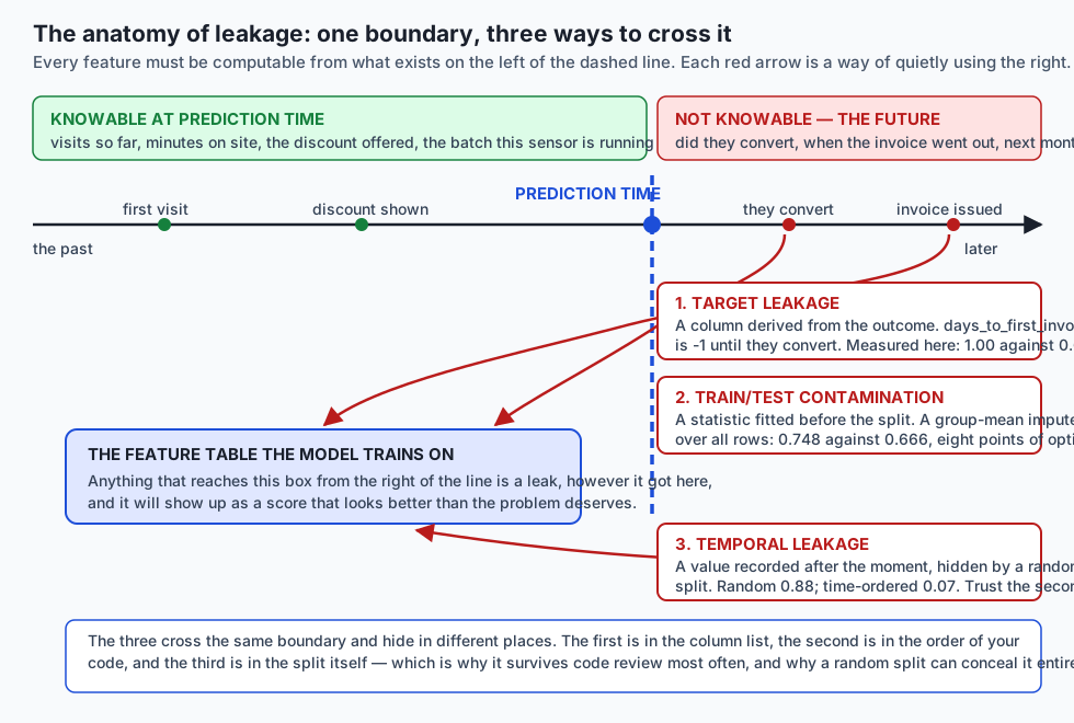
Target leakage lives in the column list. A feature encodes the outcome, directly or by proxy. You find it by reading column names and asking, for each one, “when is this written?”
Train/test contamination lives in the order of your code. Some statistic — a scaler’s mean, an imputer’s fill value, a category’s average outcome, a vocabulary — was fitted on rows the model will later be scored on. You find it by asking, of each fitted number, “which rows went into this?”
Temporal leakage lives in the split itself. Information from after the prediction moment is in the training rows, and a random split hides it completely because it scatters every period into both halves. You find it by splitting on time and watching the score fall.
The third one survives code review most often, and the reason is
structural: there is nothing to see. The column names are fine. The
fit calls are in the right order. The bug is in a line that reads
train_test_split(X, y, random_state=0), which looks like the most
innocent line in the file.
How it works
The fit/transform boundary, stated once
Every statistic you compute from data has a fitting set. Write it as two functions and the question “which rows went into this?” becomes answerable by reading the call site:
class Standardiser:
    def fit(self, X):
        self.mean_ = X.mean(axis=0)
        scale = X.std(axis=0)
        self.scale_ = np.where(scale == 0.0, 1.0, scale)
        return self

    def transform(self, X):
        return (X - self.mean_) / self.scale_
fit looks at rows. transform looks at nothing — it applies numbers
that were already decided. Once the two are separate, this line is
obviously wrong:
X = Standardiser().fit_transform(X_all)     # every row, including the test rows
X_train, X_test = X[train_idx], X[test_idx]
and this line is obviously right:
scaler = Standardiser().fit(X_all[train_idx])   # training rows only
X_train = scaler.transform(X_all[train_idx])
X_test = scaler.transform(X_all[test_idx])
That is the whole discipline. It is not subtle. It is just easy to get backwards when the preprocessing happens forty lines above the split.
Scaling, and who actually cares about it
Standardisation is Day 107’s idea: subtract the mean, divide by the standard deviation, and every column arrives at the model on comparable terms. Three families of method care about this to three different degrees:
| Method | Cares about scale? | Why |
|---|---|---|
| Distance-based (nearest centroid, k-nearest neighbours, k-means) | Enormously | The distance is a sum of squared differences. A column measured in thousands drowns a column measured in units, whatever either one means. |
| Gradient-based (logistic regression, neural networks) | Yes, through conditioning | Day 111’s condition number: badly scaled features stretch the loss surface, and a fixed step size that is stable in one direction crawls in another. |
| Threshold-based (decision trees, and anything built from them) | Not at all | A split at order_value > 240 is the same split however you rescale the axis. Monotone transformations do not move a threshold. |
That last row is worth internalising, because it is the reason “always standardise” is bad advice. Standardising before a tree costs you readability and buys nothing.
Encoding categories, and the trap in ordinal
A category is not a number, so somebody has to choose one. Three usual choices:
- One-hot: one 0/1 column per category. Honest about the absence of order, costs one column per level, and a category the training data never held becomes a row of zeros rather than a crash.
- Ordinal: replace each category with its position in a list. Correct when the order is real — small, medium, large — and a trap when it is not.
- Target encoding: replace each category with the mean outcome for that category. Compact, powerful, and the subtlest way to leak in this whole lesson.
The ordinal trap is easy to state and better to see. Take six paint colours with no order at all, and their measured return rates:
| Code | Colour | Observed return rate |
|---|---|---|
| 0 | amber | 0.230 |
| 1 | cobalt | 0.060 |
| 2 | ivory | 0.695 |
| 3 | olive | 0.145 |
| 4 | rose | 0.625 |
| 5 | slate | 0.230 |
Nothing about that column is monotone in the code — the code is alphabetical order, which is a fact about English, not about paint. Fit the same logistic regression twice, once on the ordinal code and once on the one-hot block, and ask each what it predicts for every colour:
colour   observed   ordinal   one-hot
amber      0.230     0.252     0.230
cobalt     0.060     0.281     0.060
ivory      0.695     0.312     0.695
olive      0.145     0.345     0.145
rose       0.625     0.380     0.625
slate      0.230     0.415     0.230
The one-hot model reproduces every rate to within 0.0000002. The ordinal model produces a straight line: 0.252, 0.281, 0.312, 0.345, 0.380, 0.415, climbing gently from amber to slate because that is the only shape available to it. Its worst error is 0.383 — it says ivory returns 31% of the time when ivory returns 70% of the time. Accuracy on the training data is 0.669 against one-hot’s 0.776.
That is what “imposing an order that does not exist” means concretely. The model is not confused. It is doing exactly what you asked: treating the gap between cobalt and ivory as the same size as the gap between ivory and olive, and inventing a midpoint between two colours that have none.
Target encoding, and the leak inside it
Target encoding reads the target. Say that sentence twice, because everything follows from it. If the encoding is computed before the split, every test row’s feature value was computed partly from that row’s own answer.
Take 600 rows across 40 cities — fifteen rows per city on average, which is exactly the regime where a per-city mean is mostly noise. Encode three ways and score each on the same held-out rows, averaged over forty random splits:
| Encoding | Held-out accuracy |
|---|---|
| Computed over the whole table, then split | 0.6215 |
| Computed on the training rows only | 0.5415 |
| Computed out-of-fold within the training rows | 0.5535 |
Six-point-eight points of pure fiction. And you can see the leak without a model in the way at all, by correlating each encoding with the target:
correlation of the naive all-data encoding with the target:  0.2708
correlation of the out-of-fold encoding with the target:     0.0505
The naive encoding is five times more correlated with the answer, and the extra correlation is the part it copied out of the answer.
The fix has two levels. Restricting the encoding to the training rows removes the inflation completely — the 0.5415 above. Out-of-fold encoding goes one step further: split the training rows into folds and encode each fold using the means computed from the other folds, so a row’s own target never contributes to its own feature value:
def target_encode_out_of_fold(categories, y, n_folds=5, seed=0):
    fold_of = np.random.default_rng(seed).permutation(len(y)) % n_folds
    encoded = np.empty(len(y), dtype=float)
    for fold in range(n_folds):
        held_out = fold_of == fold
        mapping, default = target_encode_fit(categories[~held_out], y[~held_out])
        encoded[held_out] = target_encode_transform(categories[held_out], mapping, default)
    return encoded
That buys back a further 1.2 points here. Out-of-fold does not excuse fitting on the test set; it is a refinement inside the training half.
Datetime features, and the cleanest small demonstration in the day
Pull a timestamp apart and you get honest features nearly for free:
hour, day of week, day of month, month, is-weekend. pandas gives you all
of them through the .dt accessor, documented in the
time series user guide.
But one of those columns is a trap in the same family as ordinal encoding. Hour is a number that wraps, and an integer column does not know that. Hour 23 and hour 0 are one hour apart in the world and twenty-three apart on the ruler — the largest gap on it, sitting exactly where the smallest one belongs.
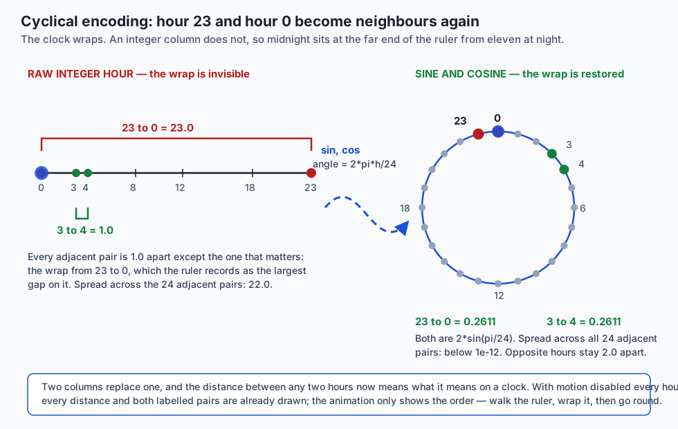
The fix is two columns instead of one — put the hour on a circle:
def cyclical_encode(values, period):
    angle = 2.0 * np.pi * np.asarray(values, dtype=float) / float(period)
    return np.column_stack([np.sin(angle), np.cos(angle)])
And now the property you wanted is checkable by distance, exactly:
raw distance, hour 23 to hour 0:        23.0
raw distance, hour 3 to hour 4:          1.0
raw spread across all 24 adjacent pairs: 22.0

circle distance, hour 23 to hour 0:      0.26105238444010315
circle distance, hour 3 to hour 4:       0.26105238444010315
circle spread across all 24 pairs:       below 1e-12
circle distance, hour 0 to hour 12:      2.0
That number is not a coincidence and not a fit: two adjacent hours are
2*pi/24 radians apart on a unit circle, so the chord between them is
exactly 2*sin(pi/24), which is 0.26105238444010315. Every adjacent
pair, wrap included, is that distance apart. Opposite hours stay 2.0
apart, the diameter. This is the rare feature-engineering decision that
you can prove correct instead of measuring, which is why it is the
cleanest demonstration in the day.
The same trick works for anything that wraps: day of week with period 7, month with period 12, day of year with period 365 — and the leap year is a genuinely annoying edge case worth thinking about rather than ignoring.
Binning, and the boundary you chose without noticing
Binning turns a continuous column into a categorical one. It can be exactly right — a threshold that matters in the domain — and it is always a decision with the same power as Day 130’s bin width.
NumPy will compute equal-width edges for you with histogram_bin_edges. Ask for three bins of a heavy-tailed column and compare against three bins of equal count:
equal-width edges:  0.81, 270.02, 539.22, 808.43
equal-count edges:  0.81,  11.13,  32.34, 808.43

top bin, equal width:   4 rows of 500, renewal rate 1.000
top bin, equal count: 167 rows of 500, renewal rate 0.563
Both are correct. Neither is wrong. And “high-value orders renew 100% of the time” and “high-value orders renew 56% of the time” are the same sentence about the same data, differing only in a boundary nobody wrote down. If you bin, say where the edges came from, and prefer edges that mean something in the domain over edges that fell out of a default.
Interactions, kept concrete
An interaction is a feature built from more than one column, expressing something neither carries alone. The two everyday forms are the ratio and the product.
Take income drawn identically for both classes, and spend equal to income times a class-dependent ratio. Neither column separates the classes, because a big spender on a big income looks like a small spender on a small one:
income alone:            0.5400
spend alone:             0.6667
spend / income:          1.0000
The ratio separates them perfectly, because the ratio is the rule.
One honest footnote, which the lab asserts rather than hides: a logistic
regression given both raw columns also reaches 1.0000 here, because
the boundary in this construction is spend = 0.5 * income, a straight
line through the origin, and a linear model can find a straight line.
The ratio is still worth building. It states the rule in one number a
person can read, it survives a change of model, and a distance-based
method gets nothing at all from the two raw columns.
Text as features, briefly
The simplest useful text feature is a bag of words: one column per word, each cell a count. The interesting decision is not the counting, it is the vocabulary — which words become columns at all — and that is a fitted statistic like any other. Fit it on the training documents.
There are two reasons, and only one of them is obvious. The obvious one: if you pick the vocabulary by association with the label, you have read the target on rows you were not allowed to read. The less obvious one: your transform must survive words it has never seen, because production will hand you plenty. Dropping an unknown token is a decision; crashing on it is a bug:
def transform(self, documents):
    position = {word: i for i, word in enumerate(self.words)}
    matrix = np.zeros((len(documents), len(self.words)), dtype=float)
    for row, document in enumerate(documents):
        for token in tokenize(document):
            column = position.get(token)      # unknown words: simply skipped
            if column is not None:
                matrix[row, column] += 1.0
    return matrix
In today’s corpus of 300 short tickets there are 79 distinct tokens, 59 of which appear in four documents or fewer. Choosing the top thirty words by correlation with the label over all documents scores 0.8137 on held-out rows; choosing them over the training documents only scores 0.7893. Two and a half points, averaged over forty splits — much smaller than the target encoding’s 6.8, and for an instructive reason. Choosing the vocabulary decides only which columns exist; a target encoding puts the leaked answer into the column’s values.
A feature’s cost
Every feature has to be computable at prediction time, from data that exists then, at acceptable expense. All three clauses bite:
- Computable at all.
days_to_first_invoicefails here. So does “average order value over the customer’s lifetime” if the prediction is made before their first order. - From data that exists then. A feature that joins a table refreshed nightly is fine for a nightly batch job and wrong for a request that must answer in 40 milliseconds with today’s data.
- At acceptable expense. A feature that needs a 200-millisecond aggregation query is not available to a system with a 50-millisecond budget, however predictive it is.
This is a systems constraint at least as much as a statistical one, and it is the constraint that a feature store is a product category to solve. Two lists are worth keeping beside your feature table: when is this value written? and what does it cost to read?
An everyday analogy
Think of a hiring panel with a scoring sheet.
The features are the questions on the sheet: years of experience, score on the exercise, whether they have shipped something similar before. Each one is a hypothesis about what predicts a good hire, and the panel’s judgement is only as good as the sheet.
Target leakage is a line on the sheet reading “still here after two years?” — filled in from the file of people who were hired years ago. It predicts a successful hire beautifully. It is also unavailable on the day you have to decide, and a panel that has grown to depend on it is worse than one that never had it, because it has stopped weighing the questions it can actually answer.
Train/test contamination is subtler. The panel calibrates: “an exercise score of 70 is about average”. Where does “average” come from? If it is computed over all of this year’s applicants — including the twenty who have not been interviewed yet, whose scores the panel has already peeked at — then the calibration is not something the panel could have had on day one. The scoring looks well-tuned in review and is not reproducible on the next batch.
Temporal leakage is a reference letter dated after the candidate started. Nobody is lying. The letter is real, and it is in the file, and if you shuffle the files and read half of them you will never notice that half your evidence post-dates the decision it is supposed to inform.
And the ordinal trap is scoring “department” from 1 to 6 in alphabetical order and then computing an average department. The number is real; the arithmetic is valid; the quantity is meaningless. Nobody is halfway between Accounting and Biology.
The analogy also carries the fix. A panel that keeps two lists — what did we know on the day? and where did each rule of thumb come from? — does not need to be clever about leakage. It has made the question answerable, which is nine-tenths of it.
Examples in practice
Everything below was measured on this machine, on 2026-08-20, with
pandas 3.0.5, NumPy 2.5.2 and Python 3.14.0. scikit-learn is not
installed, so both models are the from-scratch NumPy ones in the lab’s
models.py. The full harness output is in the lab’s
expected-output/test-run.txt.
The three leakages, in one table
| Kind | Leaky number | Honest number | Gap |
|---|---|---|---|
| Target leakage | 1.0000 | 0.6400 | 36.0 points |
| Contamination — group-mean imputer | 0.7484 | 0.6662 | 8.22 points |
| Contamination — target encoding | 0.6215 | 0.5535 | 6.80 points |
| Contamination — bag-of-words vocabulary | 0.8137 | 0.7893 | 2.45 points |
| Temporal — random split vs time-ordered | 0.8833 | 0.0667 | 81.67 points |
The surprise: contaminating a scaler bought nothing
The most instructive number in the whole day is a negative one.
Fitting a Standardiser on all the data before splitting is the
textbook example of contamination, so the lab measures it: 200 random
splits, a small 25-row test set so a single row is worth four accuracy
points, and a distance-based model that genuinely cares about scale.
scaler fitted on all data (mean of 200 splits):     0.6218
scaler fitted on training rows (mean of 200 splits): 0.6224
optimism bought by contamination:                   -0.06 points
The contaminated version scored lower. Not by much — this is a rounding error, and the honest statement is “no measurable difference” — but the expected direction did not appear at all, and it is worth understanding why.
Standardisation applies one affine map to both halves of the data.
It cannot pull the test rows towards the training rows; it moves
everything together. So contaminating it can only change the relative
weighting of the features, and a logistic regression run to convergence
is very nearly invariant to a per-feature affine reparameterisation. The
statistics really did differ — the mean of order_value is 43.94 fitted
on everything and 57.54 fitted on sixty training rows — and the score
did not care.
Two further constructions were measured before this was accepted: equal-width binning with edges fitted on all data came out 1.9 to 2.7 points in favour of the correctly fitted version, and a rank transform came out within half a point either way.
Now change the statistic to something that is not an affine map. A group-mean imputer fills each missing value with the mean of its own group. With 120 panels over 600 rows and 60% of readings missing, a group holds about five rows, and the fill value is a genuinely local piece of information:
imputer fitted on all data (mean of 150 splits):     0.7484
imputer fitted on training rows (mean of 150 splits): 0.6662
optimism bought by contamination:                     8.22 points
Eight points. Same sin, same code shape, eighty times the consequence.
The rule that survives is better than “never fit before the split”, which is true but tells you nothing about severity. It is this: a contaminated statistic is worth exactly as much as that statistic knows. A global mean and standard deviation know almost nothing about any individual row. A group mean over five rows knows a lot about those five. A category’s average target knows the answer.
The temporal one, and why it is the worst
Six calibration batches of a sensor, sixty readings each, in time order. The alarm rate per batch, measured:
B0 0.900 B1 0.083 B2 0.867 B3 0.100 B4 0.867 B5 0.067The batch is a legitimate feature — you know today which batch the sensor is running under. One-hot encode it, add the reading, fit the same model, and split the rows two ways:
random split, 60 held-out rows:         0.8833
time-ordered split, last 60 rows:       0.0667
majority-class baseline for that period: 0.9333
Read the third line again. The time-ordered model scores 0.0667 on a period where predicting the majority class would have scored 0.9333. It is not uninformed about the new batch. It is confidently wrong about it, because the one-hot column for B5 was never seen in training, the model falls back on what the earlier batches taught it, and what they taught it does not apply any more.
The random split hides this perfectly. It puts rows from B5 in both
halves, so the model learns B5’s rate from rows recorded at the same
time as the ones it is scored on, and reports 0.88. Every column name is
sensible. Every fit is in the right place. The bug is the word
random.
That gap is deliberately sharp — a rate flipping between 0.88 and 0.08 is a hard regime change, and real drift is usually milder. The durable finding is not the size. It is the sign of the comparison against the baseline: when a model meets a period it has never seen, it can be worse than knowing nothing.
The audit, and what it cannot see
Write the check once and run it on any table. Three rules, each named so a flag can be argued with:
def leakage_audit(frame, target, corr_threshold=0.90):
"""correlation | separable | pure_category"""correlation— a numeric column whose absolute correlation with the target is at or above the threshold.separable— a numeric column where a single threshold splits the classes perfectly.pure_category— a non-numeric column where every category occurs with exactly one target value.
On the signups table plus two planted columns, it flags exactly two:
days_to_first_invoice   separable       one threshold splits 'converted' without error
email_template          pure_category   every category maps to one 'converted' value
and none of visits, minutes_on_site, discount_pct or channel.
Notice which rule caught the numeric leak. Its absolute correlation with
the target is 0.8468 — under the 0.90 threshold. The correlation
rule alone would have missed it, which is the argument for the second
rule and a good reason to distrust any single-number leak detector.
And here is the honest part, which belongs in the docstring and not in a footnote: the audit reads one table at one moment. It cannot see a scaler fitted on the wrong rows. It cannot see that a column will be unavailable at prediction time. It cannot see a value backfilled from the future, or the same customer appearing on both sides of a split. It catches the loud leaks. The quiet ones are still your job.
Implications: security, privacy, performance, scalability, and cost
Security and privacy. Leakage is a confidentiality failure in statistical clothing: a channel carrying information from somewhere your production system has no access to. In a regulated setting the “can I compute this at prediction time?” question grows a third clause — and am I permitted to use it for this purpose? A feature you may join in an offline table and may not use in a live decision is a leak with legal consequences attached, and it presents exactly like every other leak: an excellent offline score. Some proxies are worse than useless even when computable: a postcode-derived feature can encode protected characteristics, and no amount of cross-validation will tell you.
Performance. Feature cost is latency. An aggregation that takes 200 milliseconds is not available to a 50-millisecond request budget, no matter how much it helps offline. Decide the budget first and let it veto features, or you will build a model you cannot deploy.
Scalability. The expensive part of a feature is rarely computing it once. It is computing it twice — once in a batch job over history and once in a request handler over live data — and having the two agree. That mismatch is called training/serving skew, and it is why the industry built feature stores rather than better libraries.
Cost. Every feature is code that must be maintained, monitored and explained. Ten features you can defend beat two hundred you cannot, and the two hundred also cost more to store, more to recompute and more to debug at three in the morning. When a feature’s contribution is inside the noise, deleting it is a real improvement.
A cost you cannot see on the invoice: a leaked result burns credibility. The team that reports 0.99 and ships 0.61 does not get the benefit of the doubt on the next number, and rightly so.
Alternatives: free, open source, and commercial
Four tools cover this ground. Two were run here. Two were not, and are described from their documentation, with no output reproduced and no pricing quoted for anything not verified.
pandas and NumPy — run here
When to choose: when the transformation is bespoke, when you want to see exactly what happened, and when the dataset fits in memory. Which is most of the time, and certainly all of this lesson.
How it is called: directly. pandas.get_dummies does one-hot
encoding in one line and is
documented here;
.dt pulls calendar parts out of a timestamp;
numpy.histogram_bin_edges computes bin edges.
import pandas as pd

frame = pd.DataFrame({"colour": ["amber", "ivory", "amber"]})
pd.get_dummies(frame["colour"], prefix="colour", dtype=float)
One caution that matters for today’s subject: get_dummies derives its
columns from the data you hand it, so calling it separately on your
training and test frames can produce different column sets. Derive
the category list once, on the training data, and pass it explicitly —
which is exactly what the lab’s one_hot does.
Free or paid: both free and open source, BSD-3-Clause. No paid tier.
scikit-learn Pipeline and ColumnTransformer — documentation only, not installed here
When to choose: as soon as you have more than one preprocessing step and any form of cross-validation. This is the tool built for the exact problem you have now felt.
How it is called: a Pipeline chains transformers and a final
estimator; when you call fit on the pipeline inside a cross-validation
fold, every transformer is fitted on that fold’s training rows only.
ColumnTransformer routes different columns to different transformers —
scale the numerics, one-hot the categoricals — and reassembles them.
Both are described in the library’s
composing estimators guide,
and the contamination problem itself is the subject of its
common pitfalls page.
# Not run in this lesson: scikit-learn is not installed on this machine.
from sklearn.compose import ColumnTransformer
from sklearn.pipeline import Pipeline
from sklearn.preprocessing import OneHotEncoder, StandardScaler
from sklearn.linear_model import LogisticRegression

pre = ColumnTransformer([
    ("num", StandardScaler(), ["visits", "minutes_on_site"]),
    ("cat", OneHotEncoder(handle_unknown="ignore"), ["channel"]),
])
model = Pipeline([("pre", pre), ("clf", LogisticRegression())])
Two details in that snippet are the whole point. handle_unknown="ignore"
is the “unseen category becomes a row of zeros” rule made explicit. And
because the scaler lives inside the pipeline, cross_val_score(model, X, y) refits it on each fold’s training rows, which is the thing you
cannot get right by hand reliably.
Free or paid: free and open source, BSD-3-Clause. No paid tier. Not installed on this machine, so no output above is reproduced.
Feast — documentation only, not installed here
When to choose: when the same feature must be computed for training over history and for serving in a request, and you need the two to agree. Feast is an open-source feature store: you declare feature definitions once, materialise them into an online store for low-latency reads, and retrieve point-in-time correct training data — that is, for each training example, the feature values as they stood at that example’s timestamp rather than as they stand now.
That last phrase is the reason a feature store belongs in a lesson about leakage. Point-in-time correctness is temporal leakage prevention turned into infrastructure. Building the same join by hand, for dozens of features, is where teams reliably introduce a value that did not exist yet.
Free or paid: the Feast project itself is free and open source (Apache 2.0). You still pay for whatever storage and compute you point it at. Not installed here; nothing above is reproduced.
Tecton — documentation only, not evaluated here
When to choose: when an organisation wants a managed version of the above — feature pipelines, an online store, monitoring and governance — rather than operating one itself.
What problem it actually addresses: the same one. Consistency between the feature computed in training and the feature computed at serving time, point-in-time correct historical retrieval, and shared definitions so two teams do not build two subtly different versions of “orders in the last 30 days”.
Free or paid: a commercial product. This lesson quotes no price, because none was verified, and pricing for products of this kind is generally negotiated rather than published. Treat any figure you see quoted second-hand as unverified.
A note on proportion: a feature store is infrastructure for an organisation with many models and many teams. If you have one model and one notebook, the fit/transform discipline in this lesson is the whole of what you need, and a feature store is an answer to a question you do not have yet.
Comparison with related concepts
| Concept | What it decides | Where it can go wrong | How today’s material relates |
|---|---|---|---|
| Data cleaning (Day 125) | What the data says | An imputation is irreversible and changes correlations | An imputer is a fitted statistic, so it can be contaminated — worth 8.2 points here |
| Pipelines (Day 126) | The order things happen in | A step that is not idempotent, a contract not checked | The fit/transform split is the pipeline contract applied to statistics |
| Feature engineering (today) | What the model is asked | A feature that encodes the answer or cannot be computed live | — |
| Feature selection | Which features survive | Selecting on all the data is contamination — the vocabulary experiment is exactly this | Choosing the top 30 words on all documents: +2.45 points of fiction |
| Model selection | Which function class | Believing a leaked score chose the model for you | Both of today’s models score 1.00 on the leaking table |
| Normalisation (Day 107) | The units | ”Always standardise” applied to trees | Distance and gradient methods care; threshold methods do not |
Three distinctions people commonly blur:
One-hot versus ordinal is not a matter of taste. Ordinal asserts an order and a spacing; one-hot asserts neither. Ask whether a midpoint between two categories means anything. If it does not, one-hot.
Target encoding versus one-hot is a trade of columns for risk. Target encoding gives you one column instead of forty, and hands you a way to leak that one-hot simply does not have.
Cross-validation versus a time-ordered split is not two flavours of the same thing. On time-ordered data, k-fold cross-validation answers a question nobody asked — how well does this do on a past it has already partly seen — and answers it optimistically.
When to use it — and when not to
Build a feature when it encodes a hypothesis you can state in a sentence, it is computable at prediction time from data that will exist then, and it survives a leakage audit and a time-ordered split.
Do not build one when:
- You cannot say when the value is written. Find out first. Half of all target leakage dies at this question.
- The data would have to come from after the prediction moment. There is no clever version of this.
- The transformation buys nothing your model class needs. Standardising before a tree, or one-hot encoding a category with 40,000 levels.
- Its cost exceeds the serving budget. A predictive feature you cannot compute in time is not a feature.
Prefer a simpler encoding when the category count is small: one-hot carries no leakage risk at all, and 40 columns is not a problem worth solving with target encoding.
Prefer target encoding when the cardinality is genuinely high — thousands of levels — and you are willing to compute it out-of-fold, smooth it towards the global mean for small categories, and re-derive it inside every cross-validation fold.
Always split on time when the data has time in it, even if you also report a random-split number. Report both. The smaller one is the honest one.
Knowledge check
Take the eight-question quiz for this day. It checks the parts people most often get half-right: why a suspiciously good score is a bug report, which of the three leakages a random split conceals, why contaminating a scaler turned out to be worth nothing while contaminating a group-mean imputer was worth eight points, what an ordinal code actually forces a model to do, and what a leakage audit cannot possibly see.
Hands-on exercise
The lab is Features That Do Not Cheat, at
labs/sections/math-statistics-and-data/day-137-thinking-in-features/.
Nine numbered exercises, each one a measurement rather than an opinion.
cd labs/sections/math-statistics-and-data/day-137-thinking-in-features
python3 -m venv .venv
.venv/bin/pip install -r requirements/requirements.txt
.venv/bin/pytest starter -v          # 9 skipped, on an untouched checkout
Open starter/test_features.py. Each test is a pytest.skip with a
docstring saying precisely which numbers to assert on. Delete the skip,
write the assertions, and run again. Read starter/00_brief.md first.
Run pytest starter and pytest examples as two separate commands.
Both directories hold a module named test_features.py, and pytest
collects by dotted module name, so a combined invocation aborts with
import file mismatch.
Expected output
An untouched checkout:
sssssssss                                                                [100%]
9 skipped
The reference answers:
.........                                                                [100%]
9 passed
The full harness, bash tests/run_tests.sh, prints every measurement
and ends with:
-------------------------------------------------------------
55 checks, 0 failure(s)
The measurements themselves, as captured here:
leak_with=1.0000
leak_without=0.6400
scaler_optimism_points=-0.0600
imputer_optimism_points=8.2233
te_naive_all=0.6215
te_out_of_fold=0.5535
time_random=0.8833
time_ordered=0.0667
time_majority_baseline=0.9333
cyc_raw_23_0=23.0000
cyc_circle_23_0=0.2611
audit_flagged=days_to_first_invoice,email_template
audit_leak_correlation=0.8468
Validate your work
bash tests/run_tests.sh; echo "exit=$?"ends with55 checks, 0 failure(s)andexit=0. Check the status directly, never through a pipe — a pipeline reports the last command’s status, not the script’s..venv/bin/pytest examples -qends with9 passed.- Your own
pytest starter -qends with9 passedonce you have finished, with no test left skipped. - Prove the suite can fail: change one assertion to something false, watch it fail, change it back. Section 6 of the harness already does this to a scratch copy.
- Compare every number you measured against
expected-output/FIELDS.md.
Troubleshooting
pytest: command not found— you have not created.venv, or you are calling a barepytest. The harness looks for.venv/bin/pytestfirst; override withPYTEST=/path/to/pytest bash tests/run_tests.sh.import file mismatch— you ran both suites in one invocation. Run them separately.ModuleNotFoundError: No module named 'experiments'— run pytest from the lab directory and name the folder,pytest starter.- The suite takes about sixteen seconds — that is where the honesty comes from. Four experiments average over 40 to 200 random splits. Do not reduce the trial counts; the assertion bands were chosen for them.
- A gap comes out with the opposite sign — one of them is meant to.
scaler_optimism_pointsis negative, andFIELDS.mdexplains why. For any other, check your NumPy and pandas versions against the pins before you touch a band.
Common mistakes
- Widening a band until the test passes. The measurement is the thing you came for. Print the dictionary the fixture gave you and look at the number first.
- Asserting an exact float where the result is a mean over random splits. Only exercise 5 is exact, because it is arithmetic rather than sampling.
- Fitting the encoder before the split “just for exploration” and then forgetting. If you want to explore, do it on the training half.
- Reading
examples/first. Every exercise is solvable from its docstring, and reading the answer first costs you the whole exercise.
Practice assignment
Take a dataset you did not build — one from Day 134’s sources is ideal — and produce a one-page feature contract for it before you model anything.
For every column, record four things:
- When is the value written? Before the prediction moment, at it, or after it. Any “after” is a leak; delete the column and say so.
- What is the fitting set for any statistic it needs? A scaler’s mean, an imputer’s fill, an encoding’s category means. Name the rows.
- Can it be computed at prediction time, and at what cost? Give a rough latency and name the system the value comes from.
- What hypothesis does it encode? One sentence. If you cannot write the sentence, you do not know what the column is for.
Then run the lab’s leakage_audit over the table and reconcile the two.
Anything the audit flagged that your contract calls honest, and anything
your contract calls a leak that the audit missed, is the interesting
part — write a paragraph on each. The mismatches are the finding.
Finish with a time-ordered split if the data has a timestamp, and report both scores with the honest one first.
Extension challenge
Break the audit, then decide whether to fix it.
Construct a feature that leaks but is not flagged by any of the three rules. Two constructions worth trying:
- A leak that lives across rows rather than within one: the same customer appearing in both halves of the split, so the model memorises the customer rather than learning the rule. No column-wise check can see this, because no column is suspicious. Measure the gap between a plain random split and a group-aware one.
- A leak that only exists within a subgroup — a column that encodes the outcome for one channel and is honest for the rest. Its overall correlation stays low and no single threshold separates the classes, so both numeric rules stay silent.
Then extend the audit to catch one of them, and measure what the extension costs in false positives on honest columns. Report both numbers. If the extension flags three honest columns to catch one leak, say so and keep the simpler rule; a check that cries wolf gets switched off, and a switched-off check catches nothing.
The habit being built here is not “write more checks”. It is that a check has a measured false-positive rate, and you should know it before you ask a team to run it.
AI thread
Most production model failures are not modelling failures.
They are a feature that was available in the training table and not at inference, or a statistic fitted on everything before the split. Both look like excellent offline results — which is precisely why an excellent offline result should raise your pulse rather than settle it. The industry’s worst hours are spent on models that were never as good as they measured, and the measurement was wrong for a reason nobody looked at because nobody had a reason to look.
This scales up rather than away. A large language model is a feature pipeline with a very expensive tail: tokenisation is an encoding decision, the context window is a feature-selection decision, and a retrieval step is a join whose point-in-time correctness nobody usually checks. Benchmark contamination — evaluation items that turn out to be in the training corpus — is target leakage at internet scale, with the same signature: a score that is better than the problem allows, and a deployed system that does not reproduce it. The response is the same one you practised today, applied to a bigger table: ask when each piece of evidence was written, and refuse to celebrate until you know.
There is a habit worth taking out of this day, and it is smaller than a methodology. When a number surprises you upwards, treat it as a defect report and go looking. Half the time you will find a leak, and you will have saved a quarter of somebody’s year. The other half you will find that the problem really was easier than you thought, and you will be able to say so with evidence instead of hope. Both outcomes are worth having. Only one of them is available to somebody who celebrated first.
Quiz
Q1. Your held-out accuracy comes back at 0.99 on a problem your team expected to be hard. What is the correct first response?
- Treat it as a bug report and go looking for a leak before telling anyone the number
- Report it, then start work on the deployment
- Re-run it with a different random seed to confirm it is stable
- Add regularisation, since a score that high indicates overfitting
Show answer
Answer: A. Treat it as a bug report and go looking for a leak before telling anyone the number
A different seed will happily reproduce a leak, so stability confirms nothing; and regularisation cannot remove information that should not be in the table at all. Overfitting shows up as a training score far above a test score, whereas leakage inflates the test score too, which is exactly why it is harder to see. The habit worth building is that an unexpectedly excellent result is evidence of a defect until you have found out otherwise -- in this lesson's lab, one column derived from the outcome moved the score from 0.64 to 1.00.
Q2. Which of the three kinds of leakage is the one a random train/test split conceals completely?
- Target leakage, because the leaking column looks like any other column
- Train/test contamination, because the fit happens before the split
- Temporal leakage, because a random split puts rows from every period into training
- All three are concealed equally by a random split
Show answer
Answer: C. Temporal leakage, because a random split puts rows from every period into training
Target leakage is visible in the column list if you ask when each value is written, and contamination is visible in the order of the code if you ask which rows fed each fitted statistic. Temporal leakage has nothing to read: the column names are sensible and every fit is in the right place. The defect is in the word random. In the lab, the same table scored 0.8833 under a random split and 0.0667 under a time-ordered one -- and the second number is the trustworthy one.
Q3. In the lab, fitting a scaler on all the data before the split was measured over 200 random splits and bought -0.06 accuracy points, while fitting a group-mean imputer the same way bought 8.22. What explains the difference?
- The scaler experiment used too few splits for the effect to appear
- Standardisation applies one affine map to both halves, so contaminating it can only change relative feature weighting, while a group-mean fill is local information about a handful of rows
- Imputation is a more advanced technique and therefore leaks more
- The scaler was fitted correctly by accident in most of the 200 splits
Show answer
Answer: B. Standardisation applies one affine map to both halves, so contaminating it can only change relative feature weighting, while a group-mean fill is local information about a handful of rows
A scaler cannot pull the test rows towards the training rows; it moves everything together, so the only thing contamination can change is the relative weighting of the features, and a logistic regression run to convergence is nearly invariant to that. A group mean over about five rows is genuinely local knowledge about those rows. The rule worth carrying is that a contaminated statistic is worth exactly as much as that statistic knows -- which also predicts why a target encoding, which knows the answer, was worth 6.8 points.
Q4. Six paint colours are encoded as an ordinal code 0 to 5 in alphabetical order and fed to a logistic regression. Their true return rates are 0.23, 0.06, 0.70, 0.15, 0.63 and 0.23. What must the model's predictions look like?
- They will match the true rates, because the model has enough capacity for six categories
- They will be identical for all six colours, because the code carries no information
- They will match for the first three colours and diverge afterwards
- They will rise or fall monotonically with the code, so they cannot match a non-monotone pattern
Show answer
Answer: D. They will rise or fall monotonically with the code, so they cannot match a non-monotone pattern
One coefficient times one number, passed through a monotone link, can only produce a monotone sequence. Measured in the lab, the ordinal model predicted 0.252, 0.281, 0.312, 0.345, 0.380 and 0.415 -- a gentle climb that is out by 0.383 on ivory. The one-hot model reproduced every rate to within 0.0000002. The failure is not a lack of capacity; it is that the encoding asserted an order, and a spacing, that the categories do not have.
Q5. You replace a high-cardinality city column with the mean conversion rate for each city, computing the means over the whole table, and then split. What have you done?
- Nothing wrong, since the encoding is only a summary of the training signal
- Given each test row a feature value computed partly from its own target
- Introduced temporal leakage, because means are computed over history
- Reduced the model's variance at the cost of a little bias
Show answer
Answer: B. Given each test row a feature value computed partly from its own target
Target encoding reads the target, so computing it before the split lets each test row contribute its own answer to its own feature. In the lab this inflated held-out accuracy from 0.5535 to 0.6215, averaged over forty splits, and you can see it without any model: the naive encoding correlates 0.2708 with the target where the out-of-fold one correlates 0.0505. Restricting the encoding to training rows removes the inflation; out-of-fold goes one better by keeping a training row's own target out of its own feature.
Q6. Why is encoding an hour as a sine and cosine pair described in this lesson as the one feature decision you can prove rather than measure?
- Because the encoding always improves model accuracy on time-stamped data
- Because two columns always beat one column
- Because the distance between any two adjacent hours becomes exactly 2*sin(pi/24), including the wrap from 23 to 0
- Because sine and cosine are bounded between -1 and 1, which standardises the feature
Show answer
Answer: C. Because the distance between any two adjacent hours becomes exactly 2*sin(pi/24), including the wrap from 23 to 0
Adjacent hours are 2*pi/24 radians apart on a unit circle, so the chord between them is exactly 2*sin(pi/24) = 0.26105238444010315 -- for every pair, wrap included, with a spread below 1e-12 across all twenty-four. Opposite hours stay 2.0 apart, the diameter. That is arithmetic, not a measurement, which is why the lab asserts it exactly rather than in a band. Whether it improves a particular model is a separate, empirical question.
Q7. A leakage audit flags a numeric column whose absolute correlation with the target is 0.85, using a threshold of 0.90. How is that possible, and what does it tell you?
- It is a bug; a 0.85 correlation cannot exceed a 0.90 threshold
- A second rule caught it -- a single threshold on the column separates the classes perfectly -- which is why a one-number leak detector is not enough
- The audit rounds correlations up to the nearest tenth
- The column was flagged as a pure category rather than as a correlation
Show answer
Answer: B. A second rule caught it -- a single threshold on the column separates the classes perfectly -- which is why a one-number leak detector is not enough
The planted leak in the lab, days_to_first_invoice, correlates 0.8468 with the target, which is under the default 0.90 threshold, so the correlation rule stayed silent. The separability rule caught it: the column is -1 for every unconverted row and at least 1 for every converted one, so one threshold splits the classes without error. Setting the threshold above 1, which disables the correlation rule entirely, still catches both planted leaks -- and no honest column is flagged either way.
Q8. Which statement about a feature's cost is the one this lesson insists on?
- A feature is worth building whenever it improves held-out accuracy
- Feature cost only matters for models served in real time, not for batch scoring
- Cost is a deployment concern and should not influence feature design
- A feature must be computable at prediction time, from data that exists then, at acceptable expense
Show answer
Answer: D. A feature must be computable at prediction time, from data that exists then, at acceptable expense
All three clauses bite independently. A feature can be computable in principle and unavailable in practice, available in a nightly table and useless to a forty-millisecond request, or predictive and too slow to read. This is a systems constraint as much as a statistical one, and the first clause is the one that would have caught days_to_first_invoice before any model was trained -- which is exactly the problem a feature store exists to make tractable at organisational scale.
Glossary
- feature
- A number given to a model, computed from data you have. Every feature encodes a hypothesis about what matters: writing spend divided by income asserts that the proportion of income being spent is the thing that carries signal, and that the same ratio means the same thing at every income level. A feature is not a column; it is a column plus a fitting procedure, because "standardised order value" is undefined until you say whose mean and whose standard deviation.
- leakage
- Information reaching the model that will not be available at the moment a prediction is actually needed. It is invisible from the inside because it makes results look better rather than worse, which is why the only reliable symptom is a score that is better than the problem allows.
- target leakage
- A feature that encodes the outcome, directly or by proxy. In this lesson's lab, days_to_first_invoice is -1 for every unconverted row and a positive number for every converted one, because an invoice cannot exist before a conversion. It takes the model from 0.64 to 1.00. This kind hides in the column list, and the question that finds it is "when is this value written?".
- train/test contamination
- Any statistic fitted on rows the model will later be scored on: a scaler's mean, an imputer's fill value, a category's average outcome, a vocabulary. It hides in the order of the code, and the question that finds it is "which rows went into this number?". Its severity varies enormously -- measured here, a contaminated scaler was worth -0.06 points and a contaminated group-mean imputer 8.22.
- temporal leakage
- Using information from after the prediction moment. It hides in the split itself: a random split scatters every period into both halves, so the model learns each period's behaviour from rows recorded at the same time as the ones it is scored on. Measured here, 0.8833 under a random split and 0.0667 under a time-ordered one, where the majority-class baseline for that period was 0.9333.
- fit/transform split
- Writing every fitted statistic as two operations: fit, which looks at rows and learns numbers, and transform, which applies numbers already learned and looks at nothing. Once they are separate, the question of which rows influenced a feature is answerable by reading the call site instead of guessing. This is what scikit-learn's Pipeline exists to enforce.
- one-hot encoding
- One 0/1 column per category, in an explicit category order derived from the training data. Honest about the absence of order, costs one column per level, and lets a category the training data never held become a row of zeros rather than a crash or a new column. Known in econometrics as dummy variables for most of a century.
- ordinal encoding
- Replacing each category with its position in a list. Correct when the order is real -- small, medium, large -- and a trap when it is not, because the code is a number and the model will read the gap between two categories as a quantity. Measured here on six unordered paint colours, the ordinal model could only produce a monotone climb from 0.252 to 0.415 and was out by 0.383 on the worst colour, where one-hot reproduced every observed rate to within 0.0000002.
- target encoding
- Replacing a category with the mean outcome for that category. Compact for high-cardinality columns and the subtlest way to leak in this lesson, because it reads the target: computed before the split, every test row's feature value is computed partly from its own answer. Usually credited to Micci-Barreca's 2001 SIGKDD Explorations paper, which prescribes smoothing towards the global mean for small categories.
- out-of-fold encoding
- Computing a target encoding for each training fold from the means of the other folds, so a row's own target never contributes to its own feature value. It is a refinement inside the training half, not a licence to fit on the test set. Worth a further 1.2 points over naive encoding on the training rows in this lesson's measurement.
- cyclical encoding
- Replacing a wrapping quantity with a sine and cosine pair, so that adjacency survives the wrap. Hour 23 and hour 0 sit 23.0 apart as integers and exactly 2*sin(pi/24) = 0.26105238444010315 apart on the circle -- the same distance as every other adjacent pair, with a spread below 1e-12 across all twenty-four. Opposite hours stay 2.0 apart, the diameter. It is the rare feature decision that can be proved rather than measured.
- binning
- Turning a continuous column into a categorical one by choosing boundaries. A bin boundary is a decision with the same power as Day 130's bin width: on the same 500 rows, equal-width edges put 4 rows in the top bin at a rate of 1.000 while equal-count edges put 167 rows in it at a rate of 0.563. Both are correct; only one of them is what you meant.
- interaction
- A feature built from more than one column, expressing something neither carries alone -- usually a ratio or a product. Measured here, income alone separated two classes at 0.54 and spend alone at 0.67, while spend divided by income separated them at 1.00.
- bag of words
- Representing a document as counts of the words it contains, one column per word. The consequential decision is the vocabulary -- which words become columns at all -- which is a fitted statistic like any other and belongs on the training side of the split. The transform must also survive tokens it has never seen, by skipping them rather than crashing.
- leakage audit
- A reusable check over a feature table and a target. The version in this lesson has three named rules: correlation above a threshold, perfect separability by a single threshold, and a non-numeric column whose every category maps to one target value. It caught both planted leaks and flagged no honest column -- and the numeric leak was caught by separability, not correlation, because its correlation of 0.8468 was under the 0.90 threshold. It cannot see contamination, unavailability at prediction time, or a value backfilled from the future.
- feature cost
- The requirement that a feature be computable at prediction time, from data that exists then, at acceptable expense. All three clauses bite independently: a lifetime average is not computable before a customer's first order, a nightly table is not current enough for a live request, and a 200-millisecond aggregation is unavailable to a 50-millisecond budget. This is a systems constraint as much as a statistical one.
- training/serving skew
- The gap that opens when the feature computed in a training pipeline and the feature computed in a request handler are not quite the same feature. It is the problem feature stores were built for, and it is the reason the same code path is worth more than the better implementation.
- point-in-time correctness
- Retrieving, for each training example, the feature values as they stood at that example's timestamp rather than as they stand now. It is temporal-leakage prevention turned into infrastructure, and it is the hardest part to build by hand across dozens of features.
Sources and further reading
- Common pitfalls and recommended practices — scikit-learn developers (accessed 2026-08-20)
- Pipelines and composite estimators — scikit-learn developers (accessed 2026-08-20)
- numpy.histogram_bin_edges — NumPy Developers (accessed 2026-08-20)
- pandas.get_dummies — pandas (NumFOCUS / pandas core team) (accessed 2026-08-20)
- Time series / date functionality (pandas user guide) — pandas (NumFOCUS / pandas core team) (accessed 2026-08-20)
Kept in this browser, no account needed. Your progress page turns the whole record into one link you can bookmark or open on another device.