Math, Statistics, and Data › Working with Real Data › Day 138
Day 138: Data Ethics, Bias, and Provenance
After this lesson you will be able to prove, with numbers rather than principles, that collecting more data does not repair a biased sampling frame: you will run a bias-versus-n ladder showing the error for an under-represented group flat at 5.94 across a hundredfold increase in sample size while the interval around it tightens 11.5-fold. You will compute a coverage mismatch against a reference distribution and report the representation ratio that names the affected group rather than the single divergence number that hides it. You will demonstrate that optimising a proxy correlated at 0.93 with its target can cut one group's share of a selection from 25% to 4% while the aggregate falls by under 2%, and that one pooled model can be worse for every subgroup than per-subgroup models. You will compute demographic parity, equal opportunity and precision for three decision policies on one calibrated population and show that no policy closes all three gaps when base rates differ -- and you will be able to state plainly why choosing among them is a value judgement to declare rather than a technical default to accept. You will count how many rows of a name-free table are unique on three quasi-identifiers, achieve k-anonymity and report what it cost in suppressed rows, and demonstrate a k-anonymous table that discloses a sensitive attribute anyway. Finally you will build a datasheet contract that names every missing provenance field, and detect a version change that every summary statistic hides.
Hands-on lab for this lesson
Lab files on GitHub: https://github.com/ai-roadmap-365/ai-roadmap-365.github.io/tree/main/labs/sections/math-statistics-and-data/day-138-data-ethics-bias-and-provenance
- Get the hands-on files. Clone the labs repository once (you can reuse this clone for every lesson). This works on macOS, Linux, and Windows (PowerShell or WSL):
git clone https://github.com/ai-roadmap-365/ai-roadmap-365.github.io.git cd ai-roadmap-365.github.io - Open this lesson's lab. Move into the directory for this specific day. Every lab lives at the same predictable path — section / subsection / week / day:
cd labs/sections/math-statistics-and-data/day-138-data-ethics-bias-and-provenance - Read the lab guide. Open `README.md` in that directory. It lists the exact commands, what each does, the expected output, and how to check your work — read it before running anything.
- Run it and check your work. Follow the README's "How to run" section: run the example first to see the finished result, then complete the numbered exercises in `starter/`, then run the tests. The tests pass (exit 0) only when your work is correct.
bash tests/run_tests.sh # or the test command named in the lab README
You can also open the lab as a local page (works offline, shows the file tree and expected output).
Learning objectives
By the end of this lesson you will be able to:
- Show that sampling bias is flat in n while sampling error falls as one over the square root of n, with measured numbers at three sample sizes
- Compute a coverage mismatch against a reference population and report a per-group representation ratio, not just a divergence number
- Name a proxy and the thing it stands in for, and measure whether optimising the proxy harms one group while the aggregate holds steady
- Demonstrate that one pooled model can be worse for every subgroup than per-subgroup models, with the wrong slope sign for both
- Compute demographic parity, equal opportunity and precision for three policies and show that no policy satisfies all three when base rates differ
- State which fairness criterion a system should satisfy as a declared value judgement, and explain why no library can make that choice
- Count rows that are unique on a small set of quasi-identifiers, and measure what generalising one field buys
- Achieve k-anonymity, report the rows suppressed to get there, and demonstrate a case where k-anonymity holds and a sensitive attribute is still disclosed
- Check a dataset against an eleven-field provenance contract that names each missing field rather than reporting a count
- Detect a version change that every summary statistic hides, and show that the provenance record is the only artifact in which it exists
- Distinguish what a licence permits from what is appropriate, and treat permitted as a floor rather than a ceiling
Prerequisites
- Day 117 -- sampling and the central limit theorem. This lesson assumes you already know that standard error falls as one over the square root of n, and turns that into the argument that bias does not
- Day 116 -- Simpson's paradox and summary statistics as lossy compression. The aggregation-bias section is that day with a decision attached
- Day 130 -- what each view of a distribution hides, and Day 132 -- chart honesty and the lie factor
- Day 134 -- source assessment, licences and provenance records. This lesson builds the datasheet that day's provenance gate was pointing at
- Comfort with pandas groupby, NumPy arrays and pytest
Why this matters
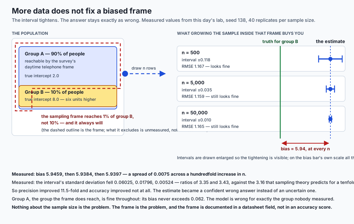
A regional statistics office runs a labour-force survey by telephone, on weekdays, between nine and five. The population it describes is 90% group A and 10% group B. The frame it actually reaches is 99% group A and 1% group B, because group B’s shift patterns put them somewhere else at the times the phone rings.
Nobody lied. Nobody was careless. The survey is well run, the response rate is respectable, the file is clean and tidy and passes every check on Day 134’s list. You fit a model on it. The in-sample RMSE is 1.17, against noise the data was generated with a standard deviation of 1.0 — a model that is doing about as well as anything could. Every dashboard is green.
The model’s prediction for group B is wrong by 5.94 units.
Here is the part that should stop you. The obvious response — get more data — does not help. Run the survey ten times harder and gather 5,000 rows instead of 500, and the bias for group B is 5.94. Run it a hundred times harder and gather 50,000 rows, and the bias for group B is 5.94. These are measured numbers from this day’s lab, forty replicate samples at each size:
| Sample size | Bias for group B | Interval half-width | In-sample RMSE |
|---|---|---|---|
| 500 | 5.9459 | ±0.118 | 1.1671 |
| 5,000 | 5.9384 | ±0.035 | 1.1593 |
| 50,000 | 5.9397 | ±0.010 | 1.1649 |
Across a hundredfold increase in sample size, the bias moved by 0.0075 — less than a seventh of one percent of itself. Meanwhile the standard deviation of the estimate fell from 0.06025 to 0.00524, ratios of 3.35 and 3.43 per tenfold step, against the 3.16 that sampling theory predicts. Precision improved 11.5-fold. Accuracy improved not at all. What you bought with all that extra data was a confident wrong answer instead of an uncertain one.
That is Day 117’s distinction between sampling error and sampling bias, and it is worth restating in the harshest available form: sampling error shrinks as 1/sqrt(n); sampling bias does not shrink at all. No amount of data fixes a frame. The frame is a decision somebody made about who to call, and it is still in the file.
This is why today is not a lesson about principles. Principles are easy to nod at and impossible to check. Every claim in this lesson is either something you can compute — a divergence, a ratio, a count of unique rows, three fairness metrics that provably cannot all be zero — or something you can write down and audit. Where a question genuinely is a value judgement rather than a calculation, and one of them is, this lesson will say so explicitly rather than pretend arithmetic settles it.
The through-line is one sentence: data is not found, it is made — by someone, for a purpose, under constraints — and every one of those decisions is still in the file. Your job is to find the decisions, measure the ones that are measurable, and document the rest where the next person will trip over them.
The idea in plain language
There is a comfortable mental model of a dataset: it sits out there in the world, someone goes and gets it, and now you have it. Everything today argues against that model.
A dataset is a record of decisions. Someone decided what counted as an observation. Someone decided who to ask and when. Someone decided which field to record and what to record in it when the true answer did not fit. Someone decided which rows to drop. Every one of those decisions is baked into the numbers, and almost none of them are visible in the numbers.
Five of those decisions go wrong in recognisable ways, and it is worth being able to name which one you are looking at, because the fix for each is different.
Selection and coverage bias enters at collection. The sampling frame — the list of things you could possibly have sampled — is a claim about who is in the world. When it is wrong, everything downstream is wrong in a way that more sampling cannot repair. This is the failure the lesson opened with, and it is measurable whenever you have a reference distribution to compare against.
Measurement bias enters at recording. The proxy is not the thing. Arrests are not crimes. Clicks are not interest. A billed diagnosis code is not a disease. Prior spending on care is not need for care. Every one of those proxies is correlated with what you actually want, often strongly, and every one of them differs from it systematically in a way that varies by group.
Historical bias is already there before anyone collects anything. The data can be a perfectly accurate record of an unjust process. A model that fits it beautifully reproduces the injustice faithfully, and the accuracy score will be excellent, because reproducing the past accurately is exactly what a high accuracy score means. This is the one where measurement genuinely runs out, and this lesson will not pretend otherwise.
Aggregation bias enters at modelling. One model for a heterogeneous population can be wrong for every subgroup in it while looking right overall. That is Day 116’s Simpson’s paradox with a decision attached to it.
Disclosure risk is not a bias at all, but it enters the same pipeline at the same points, and it is the one people are most confident about while being most wrong. “Anonymised” is not a property of a file. It is a claim about a threat model, and a small number of ordinary facts about a person is frequently enough to single them out of a table carrying no names.
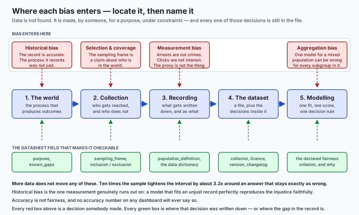
Sitting underneath all five is provenance: who collected this, when, why, under what definitions, with what inclusion criteria, and what changed between versions. A dataset without provenance is not a dataset. It is a rumour with columns. You cannot cite it, cannot re-fetch it, cannot tell whether last month’s copy and this month’s copy describe the same population, and cannot answer the single most useful question a reviewer will ask you: who is missing from this, and how would you know?
And here is the shape of the failure the opening table describes, drawn out:
Historical background
The documentation practices this day is built around are recent; the disclosure and fairness results underneath them are older.
Simpson’s paradox is the oldest thread. The reversal was described by Udny Yule in 1903 and analysed by Edward H. Simpson in a 1951 paper in the Journal of the Royal Statistical Society; the paradox carries Simpson’s name, which is why some statisticians insist on calling it the Yule–Simpson effect. Day 116 covered it as a fact about tables. Today it is a fact about models.
k-anonymity was introduced by Latanya Sweeney in 2002, formalising a decade of work on re-identification from public records. Its definition is deliberately simple: a released table is k-anonymous if every combination of quasi-identifiers that appears at all appears at least k times. Its limits were identified almost immediately, and the mid-2000s produced l-diversity as a direct response to the homogeneity problem this lesson demonstrates in exercise 7 — a class can satisfy k-anonymity and still disclose a sensitive attribute if every member of it shares the same value.
Differential privacy arrived from a different direction in 2006, in work by Cynthia Dwork, Frank McSherry, Kobbi Nissim and Adam Smith. Where k-anonymity is a property of a released table, differential privacy is a property of an algorithm: the guarantee is that the output is almost as likely whether or not any one individual’s record is present. That is a strictly stronger and structurally different kind of promise, and it is why the two are not interchangeable.
The fairness impossibility results are from the mid-2010s, when risk-scoring systems in criminal justice and lending came under sustained statistical scrutiny. Jon Kleinberg, Sendhil Mullainathan and Manish Raghavan in 2016 and Alexandra Chouldechova in 2017 independently established, in different formulations, that when base rates differ between groups, calibration and equal error rates cannot both hold except in degenerate cases. This is not a conjecture and not an empirical observation. It is arithmetic, and this day’s lab reproduces it numerically on a twenty-row table you can check by hand.
Datasheets for Datasets — the practice this day’s deliverable is modelled on — was proposed by Timnit Gebru, Jamie Morgenstern, Briana Vecchione, Jennifer Wortman Vaughan, Hanna Wallach, Hal Daumé III and Kate Crawford, first posted to arXiv on 23 March 2018 and revised through December 2021. The analogy in the paper is exact and worth keeping: in the electronics industry every component ships with a datasheet describing its operating characteristics, test results and recommended uses, and the authors propose that every dataset ship with a document describing its motivation, composition, collection process and recommended uses. Model cards, a parallel practice for documenting trained models rather than datasets, followed in 2019.
The legal vocabulary runs alongside. The Belmont Report (1979, United States) set out respect for persons, beneficence and justice as the principles governing research on human subjects, and its influence on institutional review is why “we collected it for one study and reused it for another” is a sentence that makes ethics boards uncomfortable. The GDPR was adopted in 2016 and became applicable on 25 May 2018, and its purpose limitation principle — data collected for specified, explicit and legitimate purposes may not be further processed in a manner incompatible with those purposes — is the same idea with an enforcement mechanism attached.
What is striking about this list is how much of it predates the current wave of machine learning and how little of it was routine practice when that wave arrived. The documentation gap the Datasheets paper opens by naming — that the field had no standardised process for documenting datasets — was accurate in 2018 and is only partly closed now.
What it is — and what it is not
Data ethics, as this lesson uses the term, is the practice of finding the decisions embedded in a dataset, measuring their consequences where they are measurable, and documenting them where they are not.
It is three concrete things:
- A set of measurements — coverage divergence, representation ratios, bias-versus-n ladders, per-subgroup error comparisons, fairness metric triples, uniqueness counts, k-anonymity levels — that turn vague unease into numbers you can put in a report and someone else can reproduce.
- A set of documentation artifacts — a datasheet, a data dictionary, a provenance chain with versions and a changelog — that record the decisions no measurement can recover.
- A discipline of declaring the value judgements you made, so that the next person can disagree with them explicitly instead of inheriting them silently.
It is not a checklist you can complete. Failing a check does not disqualify a dataset; it means the dataset needs a stated caveat rather than a silent assumption. Passing every check does not certify a dataset as fair, because historical bias passes every check by construction.
It is not a synonym for compliance. A licence that permits a use is a floor, not a ceiling. “Permitted” and “appropriate” are different words. A dataset released under CC0 can be used for anything the licence allows and still be entirely wrong to use for a particular purpose, because the licence says nothing about who is in it, who consented to what, or what the data was collected to measure.
It is not a technical property of a model. There is no accuracy number, no F1 score, no AUC that encodes any of this. A model that scores 0.97 on a test set drawn from the same biased frame as its training set scores 0.97 precisely because the test set inherits the same frame. The score is measuring agreement with the frame, not agreement with the world.
And it is not something a library decides for you. Fairlearn and AIF360 both compute fairness criteria accurately and well. Neither of them can choose which criterion your system should satisfy, because that choice depends on what the system is for and who bears the cost of a wrong decision, and it is a question about values rather than about statistics.
Why it was created and what problems it solves
Every practice in this lesson exists because a specific failure mode kept recurring, and each one is worth naming with its failure attached.
The datasheet exists because institutional memory is a myth. The person who chose the inclusion criteria leaves. The reason a region was excluded was obvious in the meeting and appears nowhere in the file. Two years later somebody joins two versions of the dataset on a shared key and produces a chart with a step change in it, and nobody left in the building knows whether that step is a real change in the world or a change in what was being counted. The datasheet is the artifact that answers that, and it costs almost nothing to write at the time and is essentially impossible to reconstruct later.
The coverage check exists because “national” is a word, not a measurement. A dataset titled national labour statistics that is missing one region entirely looks identical, in every visible way, to a dataset in which that region legitimately has zero of whatever is being counted. The only thing that distinguishes them is a comparison against an external reference, by name, region by region.
The proxy discipline exists because optimising a proxy is the default behaviour of every system anyone builds. The moment a number becomes a target, whatever is easiest to record about it becomes the thing being maximised. If the recorded number under-represents a group’s true state, the system will systematically under-serve that group — and the aggregate will barely move, which is exactly why nobody notices. In this day’s lab, ranking by a proxy that records one group’s need at 85% of its true level cut that group’s share of a selection from 25% to 4%, while the total need served fell by only 1.7%.
The fairness metric triple exists because “is the model fair?” is not one question. It is at least three, and they conflict. Before the impossibility results were widely understood, two well-meaning teams could each declare a system fair, on defensible grounds, and be talking past each other completely. Computing all three metrics and reporting all three is what converts that argument into a decision.
The uniqueness count exists because “we removed the names” is not anonymisation. It is a step in the direction of anonymisation whose effect is measurable and is usually much smaller than people expect. In this day’s lab, a table with no name, no address and no identifier still has 2,723 of its 5,000 rows uniquely determined by birth year, postcode and sex.
Version drift detection exists because the summary statistics you would naturally compare can be bit-for-bit identical while the population changed. Exercise 9 constructs exactly that: two releases whose count, mean, standard deviation, minimum, median and maximum are all identical, while a quarter of the sample changed group. The only place the change exists is in the changelog.
How it works
This section builds each measurement from first principles, with the numbers from a real run. Every value below came out of this day’s lab on 2026-08-20, seeded so you can reproduce it exactly.
Bias versus variance, as a ladder
Construct a world. Group A is 90% of the population with a true relationship y = 2.0 + 1.0x; group B is 10% with y = 8.0 + 1.0x. Same slope, same noise, six units of intercept apart. The sampling frame reaches group B with probability 0.01 rather than 0.10.
Fit one pooled least-squares line, ignoring the group column. Because both groups share a slope, the fitted slope is right and the fitted intercept lands at approximately 2.0 + 6.0 × p_B, where p_B is group B’s share of the sample, not of the population. With p_B = 0.01, that is 2.06. So the predicted value for a group B member is off by 2.06 - 8.0 = -5.94, at every x.
That number is not an artifact of the sample size, because p_B is a property of the frame. It is the same at n = 500 and at n = 50,000. Run it forty times at each size and you get the measured table from the opening: bias 5.9459, 5.9384, 5.9397; standard deviation 0.06025, 0.01796, 0.00524.
Both parts are worth taking seriously. The standard deviation falling by 3.35× and 3.43× per tenfold step is sampling theory behaving exactly as advertised — the prediction is sqrt(10) = 3.162, and the small excess is the finite-replicate noise of estimating a standard deviation from forty draws. The bias staying at 5.94 is the thing no amount of that behaving-as-advertised can touch.
And group A is fine. Its bias never exceeds 0.062. The pooled model is wrong for exactly the group nobody measured, and right for the group who filled the training set. That asymmetry is the whole story of the day in one line.
Coverage mismatch, computed
Given a reference distribution — a census, a published statistical abstract, anything external that states what the population looks like — the mismatch stops being a worry and becomes a subtraction.
Two numbers, and the order matters. The total variation distance between the sample’s share vector and the reference’s is half the sum of absolute differences. For this day’s survey fixture it is 0.089583. That is real, and it is small enough to be reassuring, which is precisely why it is the wrong number to lead with.
The number that names the problem is the representation ratio per group: sample share divided by reference share. The four regions come out at 1.094, 1.101, 1.111 and — for the west — 0.104167. The west appears at roughly a tenth of the rate the population says it should. That is one number, attached to one name, and it is the sentence you put in the report.
sample_shares = {g: count / total for g, count in sample_counts.items()}
ratios = {g: sample_shares[g] / reference_shares[g] for g in reference_shares}
tvd = 0.5 * sum(abs(sample_shares[g] - reference_shares[g]) for g in reference_shares)
flagged = [g for g, r in ratios.items() if r < 0.5 or r > 2.0]
Four lines. There is no library needed and no excuse for not running it.
The proxy gap, measured
Take a population where both groups are drawn from the same true-need distribution, so any fair procedure would select them in proportion to their size. Record need through a proxy that captures group A’s need faithfully and group B’s at 85% of its true level, plus noise.
The proxy correlates with the target at 0.9253. It passes the check most people run.
Now spend a fixed budget: select the top 500 of 4,000 by proxy, and separately the top 500 by true need. Ranking by the target selects group B at 0.2500 — its exact population share. Ranking by the proxy selects group B at 0.0400. Group B’s true need served falls to 0.1785 of what a target-ranked selection would have delivered.
And the total need served falls only to 0.9831 of the target-ranked total. Under a 2% aggregate degradation, one group lost 82% of what it should have received. That gap between the aggregate view and the group view is the entire mechanism by which measurement bias survives review.
The procedural fix is not statistical. It is: name the proxy and name the thing it stands in for, in writing, before you optimise it. Arrests, offences. Clicks, interest. Billed codes, disease. Prior spend, need. Once the pair is written down, the question “does this proxy differ systematically by group?” becomes askable, and it is frequently answerable from data you already have.
Aggregation bias, with stakes
Two subgroups. Group A lives at low x with a low intercept; group B at high x with a much higher one. Both trend downward — true slopes measured at -0.9870 and -0.9991.
Fit one pooled line and the slope comes out at +1.9785. Not merely imprecise: the wrong sign, for every subgroup in the data. The pooled model’s RMSE is 5.0275 for group A and 5.0545 for group B, against per-subgroup fits of 1.0192 and 1.0040. It is worse for every subgroup, not worse on average — a distinction that matters, because “worse on average” invites the reply “but it’s better for most people”, and here there is no most people for whom it is better.
The fairness tension, demonstrated
This is the section where the arithmetic stops being able to tell you what to do, and it is important to see exactly where that happens.
Build a population by hand so nothing is estimated. Two groups of 1,000. Each person carries a risk score in 0.1, 0.3, 0.5, 0.7, 0.9, and in every score bin exactly that fraction is positive. Group A’s mass sits high, group B’s sits low:
| Score | Group A count | Group A positives | Group B count | Group B positives |
|---|---|---|---|---|
| 0.1 | 50 | 5 | 350 | 35 |
| 0.3 | 100 | 30 | 300 | 90 |
| 0.5 | 200 | 100 | 200 | 100 |
| 0.7 | 300 | 210 | 100 | 70 |
| 0.9 | 350 | 315 | 50 | 45 |
| Total | 1,000 | 660 | 1,000 | 340 |
Every positives figure is a whole number, so nothing here is rounded. The score is perfectly calibrated for both groups — the maximum deviation between the score and the observed positive rate is exactly zero. Base rates are 0.66 and 0.34. That single difference is the engine of everything that follows.
Three decision policies, three criteria. Demographic parity asks that both groups be selected at the same rate. Equal opportunity asks that both groups’ genuinely-positive members be selected at the same rate — equal true-positive rates. Predictive parity, which is calibration applied to the decision rather than the score, asks that the selected people in both groups be positive at the same rate — equal precision.
| Policy | Selection rate A / B | True-positive rate A / B | Precision A / B |
|---|---|---|---|
| One threshold at 0.5 | 0.8500 / 0.3500 | 0.9470 / 0.6324 | 0.7353 / 0.6143 |
| Equalise selection rate | 0.6000 / 0.6000 | 0.7424 / 0.8529 | 0.8167 / 0.4833 |
| Equalise true-positive rate | 0.6560 / 0.5400 | 0.8000 / 0.8000 | 0.8049 / 0.5037 |
Read down the bolded cells. Each policy closes its own gap exactly — to zero, not approximately — and opens at least one other. The single threshold preserves the calibrated score untouched and produces a 0.50 parity gap and a 0.31 opportunity gap. Enforcing parity drives the selection-rate gap to 0.0000 and pushes the precision gap out to 0.3333. Enforcing equal opportunity drives the opportunity gap to 0.0000 and pushes the parity gap to 0.1160 and the precision gap to 0.3012.
No policy closes all three. That is not a failure of these three policies. It is the impossibility result, reproduced on twenty numbers you can add up yourself, and it holds whenever base rates differ.
Now the part that must be said plainly. Which criterion your system should satisfy is a value judgement, not a technical detail. It depends on what the system does, what a false positive costs the person it lands on, what a false negative costs them, whether the base-rate difference is itself the product of the historical bias you are trying not to reproduce, and who has standing to object. Reasonable, well-informed people disagree about it in good faith, and the disagreement is genuine rather than a symptom of somebody not having read the maths.
What is not a matter of opinion is that you must choose, that the choice must be written down, and that a library default is not a choice. The most common failure here is not picking the wrong criterion. It is picking one by accident, by using whatever a function returned first, and never telling anyone.
Uniqueness, k-anonymity, and where the technique stops
Build a synthetic register of 5,000 rows: birth year, postcode, sex, and a diagnosis. No name. No address. No identifier of any kind.
Count the rows that are the only row with their combination of the first three fields. The answer is 2,723 — 54.46% of the table. Over half of these people can be singled out by anyone who knows three ordinary facts about them.
Coarsen one field: exact birth year becomes a ten-year band. Count again: 13. A reduction factor of 209.5, from one edit.
keys = ["birth_year", "postcode", "sex"]
sizes = frame.groupby(keys, observed=True)[keys[0]].transform("size")
uniques = int((sizes == 1).sum())
k-anonymity is the same groupby read differently: the table’s k is the size of its smallest equivalence class. After generalisation this register’s k is still 1 — generalisation alone does not get you there. Suppressing every class smaller than 5 does, at a cost of 794 rows, roughly one in six people, and every one of them somebody in an unusual combination. Say that cost out loud when you report the k, because the rows suppression removes are frequently the people the analysis was supposed to be about.
And then the limit, which matters more than the technique. Here is a table that is 4-anonymous by construction:
| Birth decade | Postcode | Sex | Diagnosis |
|---|---|---|---|
| 1970 | 1001 | F | diabetes |
| 1970 | 1001 | F | diabetes |
| 1970 | 1001 | F | diabetes |
| 1970 | 1001 | F | diabetes |
Every equivalence class has four members, so k = 4 and the check passes. And it discloses completely: knowing that someone is a 1970s-born woman in postcode 1001 who appears in this table reveals her diagnosis exactly. No re-identification was required. Membership in the class was enough, because the class is homogeneous in the sensitive attribute. That is the observation l-diversity was invented to address, and l-diversity has its own next limit in turn.
The lesson is not that k-anonymity is useless. It is that a check trusted past its stated guarantee is worse than no check, because it buys confidence it did not earn.
The datasheet, as an executable contract
The deliverable of the day is a document, and the way to keep a document honest is to make a test fail when it is incomplete.
Eleven fields, chosen because each answers a question that cannot be recovered from the data once it is lost: collector, collection_period, purpose, population_definition, sampling_frame, inclusion_criteria, exclusion_criteria, known_gaps, licence, version, changelog.
The check must report the missing fields by name. “Documentation incomplete” is not actionable; “no exclusion_criteria recorded” is. And a field that is present but blank — an empty string, an explicit null, an empty list — counts as unanswered, because it tells a reader nothing. Against this day’s deliberately under-documented fixture the check names eight missing fields out of eleven; against the complete one it passes.
Version drift, and the thing summaries cannot show
Two releases of one dataset. The measured column is byte-for-byte identical between them, so every summary statistic matches exactly: count 2000, mean 49.9967280173, standard deviation 9.6894130750, and the same minimum, median and maximum. A reader diffing describe() output between the two releases sees nothing whatsoever.
What changed is who is in the file. Group B went from half the sample to a quarter — a composition shift of 0.2500. The only artifact in which that change exists is the provenance record: the sampling_frame field differs, and the changelog gained one line saying sampling frame re-scoped: group B quota reduced from 50% to 25%.
That is the strongest available argument for the documentation habit. It is not paperwork attached to the analysis. On this comparison, it is the only place the change exists at all.
An everyday analogy
Think of a dataset as a photograph, and carry the comparison the whole way, because every part of it maps onto something specific.
The frame is the sampling frame. A photograph shows what was inside the rectangle when the shutter opened. Everything outside it is not in the picture, and — this is the part that matters — the picture contains no evidence that anything was outside it. A crowd photographed from the front looks like a crowd, whether there were fifty people or five thousand behind the camera. A survey that called only during working hours looks like a survey, and the people who were at work are not in it, and the file does not say so. You cannot see absence.
The exposure is the proxy. A camera does not record light; it records how much a sensor responded to light, which depends on the sensor. Photograph two people of different skin tones under one exposure setting calibrated for one of them and both faces are present, both are “measured”, and one is measured much less accurately. Nobody chose that. It is a property of the instrument that nobody wrote down. Arrests as a proxy for offences works exactly this way: the instrument responds more in some places than others, and the file records the response, not the thing.
The subject is the historical process. If you photograph an unjust scene, you get an accurate photograph of an unjust scene. There is no camera setting that fixes it, and improving the camera makes the record more faithful, not less. A model trained on it does the same. This is where the analogy stops being reassuring, and it should.
The crop is aggregation. Crop two very different halves of an image into one thumbnail and the thumbnail can look like neither. Average two subgroups with opposite trends into one slope and the slope points the wrong way for both.
The caption is provenance. A photograph with no caption is not evidence of anything, however sharp it is. Who took it, when, where, and what were they trying to show? The same photograph captioned two different ways supports two different claims, and the caption is exactly the part that gets lost when a picture is reposted. Which is what a dataset without a datasheet is: a very sharp photograph with the caption torn off.
And to finish the mapping: more megapixels do not widen the frame. That is the opening result. You can shoot at ten times the resolution and everything outside the rectangle stays outside it, in more and more detail. Resolution is variance. The rectangle is bias.
Examples in practice
A survey that is right about the country and wrong about a region. The national estimate from the opening example is fine, because the region that is missing is 10% of the population and the aggregate is dominated by the 90% that is present. Every national figure the survey publishes is defensible. Every regional figure for the west is wrong by an amount nobody computed, and the only thing that would have caught it is the four-line coverage check against a published reference. The fix, once found, is not “collect more”; it is either reweighting — which trades bias for variance, and is not free — or a stated caveat naming the west explicitly, or a second collection mode. All three are decisions. All three belong in the datasheet.
A resource allocation system optimising the wrong number. A programme has budget to enrol 500 people out of 4,000 and wants to reach those with the greatest need. Need is not observed; prior engagement with the service is, and it correlates at 0.93. The programme ranks by engagement. Twelve months later the aggregate outcome is 98% of what a perfect ranking would have achieved — a genuinely good result by the metric anyone would put on the slide — and one group has received 18% of what it should have. Nobody in that process did anything wrong by their own lights. The proxy was reasonable, the correlation was checked, the outcome was measured. What was never done was disaggregating the outcome by group, which is one groupby and would have shown it immediately.
A “de-identified” release that identifies people. A hospital releases a research extract with names and record numbers stripped: age, postcode, sex, and diagnosis. The release passes the internal check, which was “no direct identifiers present”. Nobody counted uniqueness. In a table of this shape, over half the rows are singletons on the three remaining fields, and anyone who knows one of those three facts about a person — a neighbour, a colleague, an employer — can find their row and read the fourth. The generalisation that fixes most of it costs one line of code and one column of precision.
Two versions of a source, joined across the seam. A dataset is refreshed annually. This year’s release quietly changed its inclusion criterion. Every summary statistic looks stable, so the refresh passes review. Someone joins the series across the seam and produces a chart with a step change that gets described in a meeting as a shift in the underlying population. It is not. It is a shift in who was counted, and a two-line changelog entry would have made it visible in five seconds. This is the same failure Day 134 opened with, viewed from the other side: there the two definitions came from two sources, here they came from two versions of one.
Implications: security, privacy, performance, scalability, and cost
Privacy is where this day’s technical content bites hardest, and the crucial reframing is this: anonymity is a claim about an adversary, not a property of a file. Before you release anything, write down what you assume an adversary knows. Then measure: how many rows are unique on that assumed knowledge? What k do you achieve, and what did the suppression cost? Which classes are homogeneous in the sensitive attribute? Those three numbers take minutes to compute and are the difference between a release you can defend and one you merely hope about.
Treat the outputs as sensitive in their own right. “These 2,723 rows are singletons” is a map of who is easiest to identify, and it should not travel further than the release decision it informs.
Security here is mostly about provenance as integrity. Day 134’s checksum discipline is the mechanism: a provenance record carrying URL, retrieval timestamp and SHA-256 lets you prove that the file you analysed is the file the source served. Without it, “downloaded from X” is a claim rather than a proof, and a silently modified upstream file is indistinguishable from a real change in the world.
Performance is not a concern for any of these measurements, which is worth stating because “we didn’t have time” is the most common reason they are skipped. Every measurement in this lesson is a groupby, a division, or a least-squares fit. The entire nine-exercise harness — including forty replicate fits at n = 50,000 — runs in a couple of seconds. The reason these checks do not get run is not cost.
Scalability does bite in one specific place: intersectional analysis. Checking coverage across one attribute with four levels is four numbers. Across three attributes it is the product of their cardinalities, and the cells get small fast — which is both a statistical problem, because small cells give noisy estimates, and a privacy problem, because small cells are exactly the ones k-anonymity suppresses. There is a genuine tension there: the groups most likely to be harmed are often the smallest, and the smallest groups are the ones both statistics and privacy protection push you to stop looking at. There is no clean resolution. Name it, and report the cell sizes alongside the estimates so a reader can judge.
Cost is asymmetric, and the asymmetry is the argument. Writing a datasheet at collection time costs perhaps an hour of the person who already knows the answers. Reconstructing one two years later costs weeks and usually fails, because the person left. Running the coverage check costs four lines. Discovering a coverage gap after a report is published costs the report. Computing uniqueness costs one groupby. Discovering it after a release costs something you cannot buy back.
And the AI thread. A model inherits its training data’s frame, its proxies and its history, and none of that is visible in an accuracy number. This matters more, not less, as models get larger. A large model trained on a corpus assembled by whatever was cheapest to scrape has a sampling frame — an enormous, undocumented, unmeasured one — and every result in this lesson applies to it unchanged. Scaling the corpus is the same move as increasing n: it drives variance down and leaves the frame exactly where it was. You have now seen that arithmetic run, at three sample sizes, on a case simple enough to check by hand: the interval tightened 11.5-fold and the error for the under-represented group did not move. That is why the honest starting point for evaluating a model is not its score but its dataset’s documentation — and why “we don’t know what’s in the training data” is not a minor gap in a model card. It is the answer to the only question that would have told you where the model is wrong.
Alternatives: free, open source, and commercial
Four options cover this area. Two of them I ran; two I did not, and I will say which is which every time.
pandas and NumPy — the measurements themselves
When to choose it: always, and first. Every measurement in this lesson is a groupby, a value_counts, a division or a least-squares fit. Doing it yourself means you can see that the fairness incompatibility is arithmetic rather than a library’s opinion, and it means the check runs in your existing pipeline with no new dependency.
How it is called: the whole coverage check is four lines, shown earlier. The uniqueness count is one transform("size"). The k level is one min() on a group size. The three fairness metrics are counts of selected rows and selected positives per group.
selected = frame[frame["score"] >= threshold]
by_group = frame.groupby("group", observed=True)
rates = selected.groupby("group", observed=True).size() / by_group.size()
tpr = (selected.groupby("group", observed=True)["label"].sum()
       / by_group["label"].sum())
precision = (selected.groupby("group", observed=True)["label"].sum()
             / selected.groupby("group", observed=True).size())
Free vs paid: both are free and open source under BSD-3-Clause. There is no paid tier and nothing to buy.
Did I run it? Yes. NumPy 2.5.2 and pandas 3.0.5, on Python 3.14.0. Every number quoted in this lesson came out of that run, and the captured output is in the lab’s expected-output/ directory.
Datasheets and model cards — documentation practices, not software
When to choose it: for every dataset you publish, every dataset you accept from elsewhere, and every model you ship. A datasheet documents the dataset: motivation, composition, collection process, recommended uses. A model card documents the trained model: intended use, out-of-scope use, and — the part that connects to this whole lesson — disaggregated performance figures rather than a single headline score.
How it is used: there is no package to install. It is a template you fill in, checked into version control beside the data, and — this is the part that makes it stick — validated by a test. This day’s lab turns eleven required fields into an assertion that names each missing one, and that is the difference between a template people fill in and a template people mean to fill in.
missing = [name for name in REQUIRED_FIELDS
           if not str(record.get(name, "")).strip()]
assert not missing, f"datasheet incomplete: {missing}"
Free vs paid: both are published practices, free to adopt, with no licensing attached. The Datasheets paper is openly available.
Did I run it? The contract check yes — it is exercise 8 of this day’s lab and it runs. The practices themselves are described from the published paper, not from any tool.
Fairlearn — a fairness assessment toolkit
When to choose it: when you have gone past three metrics on two groups and want disaggregated analysis across several sensitive features, intersecting groups, confidence intervals on the metrics, and mitigation algorithms as well as measurement.
How it is called: its central object is MetricFrame, which computes any performance metric disaggregated by one or more sensitive features rather than as a single pooled number. On top of that it provides predefined fairness metrics — demographic parity, equalized odds, equal opportunity among them — that use MetricFrame internally and return an aggregate. Its documentation also covers intersecting groups, control features, bootstrap confidence intervals on the metrics, and a separate set of mitigation approaches organised as preprocessing, postprocessing, reductions and adversarial methods. Its user guide notes, usefully and unusually, that these metrics are “widely (if occasionally incautiously) used”, and it devotes a section to the four-fifths rule being often misapplied.
Free vs paid: free and open source under the MIT licence, maintained as a community project. There is no paid edition.
Did I run it? No. Fairlearn is not installed in this repository’s authoring environment, it was not installed for this lesson, and no output from it is reproduced anywhere here. Everything above is described from its published user guide, checked on 2026-08-20, on which date the documentation site served version 0.15.0.dev0. The three metrics in this lesson’s tables were computed with pandas, by hand, in about twenty lines — which is deliberate, because the incompatibility is a fact about arithmetic and seeing it that way is worth more than seeing it printed by a library.
Be accurate about what such a toolkit does: it computes criteria; it does not decide between them. No function in it will tell you whether your system should equalise selection rates or true-positive rates, because that is not a question a function can answer.
AIF360 — a broader fairness toolkit
When to choose it: when you want a wider catalogue of fairness metrics and mitigation algorithms than Fairlearn’s, drawn from a broad sweep of the research literature, and you are willing to spend more time working out which of them applies to your situation.
How it is called: it wraps your data in its own dataset abstraction and exposes metric classes and a set of pre-processing, in-processing and post-processing mitigation algorithms against that abstraction.
Free vs paid: free and open source under the Apache-2.0 licence, developed originally at IBM and now under the LF AI and Data Foundation.
Did I run it? No. AIF360 is not installed in this repository’s authoring environment and no output from it is reproduced anywhere in this lesson or lab. The description above is deliberately brief and structural rather than detailed, because describing an API I have not exercised in more detail than that would be guessing dressed as documentation. If you intend to use it, read its own documentation rather than this paragraph.
Both toolkits are worth knowing about and neither is a prerequisite for doing this work well. If you can compute three metrics with groupby and write down which one you chose and why, you are already doing the substantive part.
Comparison with related concepts
| Concept | What it is | What it is not | Where it bites |
|---|---|---|---|
| Sampling error | Random variation between samples | Something you can wish away | Falls as 1/sqrt(n); more data really does fix it |
| Sampling bias | Systematic mismatch between frame and population | A small-sample problem | Flat in n; 100× more data moved it by 0.13% |
| Accuracy | Agreement with the labels you have | Agreement with the world | High accuracy on a biased frame is a measure of the frame |
| Fairness | A choice among conflicting criteria | A single number | Three criteria; at most one can be exactly zero when base rates differ |
| k-anonymity | Every quasi-identifier class has at least k members | A guarantee about what those members have in common | A homogeneous class discloses at any k |
| Differential privacy | A property of the algorithm producing the output | A property of a released table | Guarantees hold against an adversary with arbitrary side information |
| Data dictionary | What each column means | Why the dataset exists or who is in it | Catches definition mismatches between columns |
| Datasheet | Why, by whom, about whom, with what gaps | A licence, or a data dictionary | Catches frame changes, purpose creep and coverage gaps |
| Model card | What a trained model is for and where it fails | A substitute for a datasheet | Disaggregated performance, out-of-scope uses |
Three of these comparisons repay a second look.
Bias versus variance is the one this day is built on, and the reason it is worth restating in this form is that the everyday intuition “more data is better” is correct for variance and completely wrong for bias, and the two are usually discussed together in a way that lets the first swallow the second.
Anonymisation versus pseudonymisation is the distinction most often collapsed. Replacing a name with a stable identifier is pseudonymisation: it removes the direct identifier and preserves the ability to link rows across releases, which is often exactly what you wanted and is also exactly what makes re-identification tractable. Anonymisation is a claim that no individual can be singled out at all, and it is a claim you have to substantiate with a measurement, not assert by having deleted a column.
Datasheet versus data dictionary is the pairing Day 134 set up and this day completes. The dictionary tells you what a column means — the thing that catches two same-named columns with different definitions. The datasheet tells you what the dataset is: who made it, why, about whom, with what gaps. You need both, and having one is no evidence of the other.
When to use it — and when not to
Run the coverage check whenever a reference distribution exists. It costs four lines and it is the single highest-yield check in this lesson. If no reference exists, say so in the datasheet’s known_gaps field rather than quietly proceeding — “we have no external reference for this population’s composition” is a real and useful finding.
Run the bias-versus-n ladder when someone proposes collecting more data to fix a quality problem. It is fifteen lines and it settles the argument. If the problem is variance, more data fixes it and the ladder shows it. If the problem is the frame, the ladder shows that too, and it shows it in a way nobody can talk past.
Disaggregate every outcome metric by group, always. This is the cheapest habit in the lesson and prevents the most common failure. A pooled metric that looks fine is compatible with an arbitrary amount of subgroup harm.
Compute all three fairness metrics whenever a model makes decisions about people — and report all three, even, especially, when you have a preferred one. Reporting only the criterion your system happens to satisfy is not analysis; it is advocacy with a table attached.
Measure uniqueness before every release of individual-level data, without exception, and record the k you achieved and the rows you suppressed to get there.
Write the datasheet at collection time. Not later. There is no later.
Now the honest boundaries.
Do not present a fairness metric as a verdict. Three numbers, a stated choice and the reasoning behind it is analysis. One number labelled “fair” is a claim you cannot support, and it will be believed.
Do not use k-anonymity as a release gate on its own for genuinely sensitive attributes. Check for homogeneous classes as well, and for high-risk data consider whether a differentially private release mechanism is the right instrument instead. And note that this lesson has described differential privacy rather than demonstrated it: no differentially private mechanism was implemented or run here, and you should read its own literature before relying on it.
Do not treat a licence as an ethics review. Permitted is a floor. A CC0 dataset of people’s search queries is legally reusable and may still be entirely wrong to reuse, because the people in it did not agree to be in your project and the licence did not ask them.
Do not skip the analysis because the topic is uncomfortable. The most common failure mode in practice is not a wrong measurement; it is no measurement, on the grounds that the question feels political. Every quantity in this lesson is a subtraction or a groupby. The measurable parts should be measured, precisely so that the genuinely contested parts — which criterion, what a false negative costs, whether a base-rate difference is itself an artifact of the history — can be argued on their merits instead of being confused with the arithmetic.
And do not claim more than you measured. If you did not check coverage, say you did not. If your reference distribution is itself from a source with its own frame, say that. The whole value of this discipline is that it makes claims checkable, and an unsupported claim in a document full of checkable ones is worse than the same claim on its own, because it borrows credibility it has not earned.
Knowledge check
Work through these before opening the lab. Each has a definite answer that follows from something in this lesson.
- A model’s error for one subgroup is 5.94 at n = 500 and 5.94 at n = 50,000, while the standard deviation of that error fell by a factor of 11.5. Which quantity is bias and which is variance, and which one does collecting more data address?
- A coverage check returns a total variation distance of 0.0896. Why is that number, on its own, a poor thing to lead a report with, and what should you report beside it?
- A proxy correlates with its target at 0.93 and the aggregate outcome under proxy-ranked selection is 98% of optimal. Explain how one group can nevertheless have received 18% of what it should have.
- A pooled model’s RMSE is worse for group A and worse for group B than per-group models. Why is that a stronger statement than “worse on average”?
- A classifier is perfectly calibrated for both groups and the groups have different base rates. What can you conclude, without computing anything, about whether it satisfies demographic parity?
- A table with no names has 2,723 of 5,000 rows unique on three quasi-identifiers. What does removing the names actually accomplish, and what does it not?
- A released table is 5-anonymous. Name a way it can still disclose a sensitive attribute, and say what check would have caught it.
- Two dataset versions have identical count, mean, standard deviation, minimum, median and maximum for their measured column. Name a change that is fully compatible with all six of those being identical, and name the artifact that would reveal it.
Hands-on exercise
Build and run the nine measurements from this lesson: labs/sections/math-statistics-and-data/day-138-data-ethics-bias-and-provenance/.
cd labs/sections/math-statistics-and-data/day-138-data-ethics-bias-and-provenance
python3 -m venv .venv
.venv/bin/pip install -r requirements/requirements.txt
.venv/bin/pytest starter -v
Read starter/00_brief.md for the nine exercises in full, then open starter/test_ethics.py and replace each pytest.skip(...) with real assertions. Exercise 1 is the centrepiece: prove that the bias for the under-represented group is flat across a hundredfold increase in n while the variance falls as sampling theory says it should. Exercise 5 is the one to slow down on: assert the incompatibility, not a preferred criterion.
Every dataset in the lab is synthetic and constructed from a seeded generator. That is deliberate, and the lab says so in three places. A lesson about who is missing from a dataset should not be taught on records describing people who never agreed to be in one — and a constructed population has a property no real one has: its true composition is known exactly, so “under-represented by a factor of ten” is a fact you can assert rather than an impression you can argue about.
Expected output
On an untouched checkout, pytest starter -v reports 9 skipped, each skip message naming exactly what to assert. Once every exercise is solved it reports 9 passed, which is what .venv/bin/pytest examples -q already reports before you touch anything, since that directory is the solved version.
The full harness ends with 51 checks, 0 failure(s) and exits 0. The captured run, including every measured value quoted in this lesson, is in the lab’s expected-output/test-run.txt, and expected-output/FIELDS.md records which figures are exact everywhere and which are pinned to NumPy 2.5.2 and seed 138.
Validate your work
Run the full harness from the lab directory:
bash tests/run_tests.sh
echo "exit=$?"
Confirm the exit code directly with echo $? immediately afterwards, never through a pipe — a pipeline reports its last command’s status, so bash tests/run_tests.sh | tail -3 followed by echo $? reports tail’s success and can hide a completely failing run underneath it.
Section 6 of the harness proves the suite can genuinely fail: it copies the solved suite to a scratch directory, confirms green, rewrites exercise 6’s exact uniqueness count from 2_723 to 9_999, confirms a non-zero exit and a printed failure, restores the file, and confirms green again.
Troubleshooting
See troubleshooting.md in the lab directory for the full list. The three most common. Running pytest examples starter in one command aborts with an import file mismatch, because both directories define a module named test_ethics.py — always run them as two separate commands, and the harness asserts that this collision happens so the trap is proven rather than merely mentioned. A version mismatch: numpy pinned 2.5.2 failure on the very first check means the pins are not installed, and every numeric assertion in exercises 1, 3, 4, 6 and 7 is tied to a specific NumPy random stream, so that is a real reason to stop. And exercise 5 feeling like it must have a right answer is the exercise working, not failing.
Common mistakes
Fitting a per-group model somewhere in exercise 1 and getting a bias near zero — the whole point is that the pooled model is the one everybody actually fits. Leading with the total variation distance in exercise 2 and treating 0.0896 as reassuring, when the representation ratio of 0.104 for one region is the finding. Reporting only the aggregate in exercise 3, where the aggregate falls by 1.7% and one group loses 82% of what it should have had. Reading exercise 4’s result as “the pooled model is a bit worse”, when it has the wrong sign for every subgroup. And, most consequentially, adding an assertion to exercise 5 that one of the three policies is correct — that is a value judgement the arithmetic cannot settle, and the exercise asks you to write your reasoning in a comment instead. That comment is the artifact the day is asking you to produce.
Practice assignment
Write a complete datasheet for a dataset you actually use — one from work, from a course project, or one you downloaded during Day 134. Fill in all eleven fields honestly: collector, collection period, purpose, population definition, sampling frame, inclusion criteria, exclusion criteria, known gaps, licence, version, changelog.
Then measure what you can. If a reference distribution exists for the population it claims to describe, run the four-line coverage check and record the representation ratio for every group, not just the total variation distance. If the data is at individual level, count how many rows are unique on the three or four quasi-identifiers a plausible adversary would know, and report the number. If any column is a proxy, name the proxy and the thing it stands in for in one line each, and say whether you have any evidence about whether the gap between them varies by group.
The finding is not the completed document. The finding is the fields you could not fill in. Write a closing paragraph listing them, and for each one, state what you would have to do to answer it and who you would have to ask. That paragraph is the honest deliverable, and it is frequently more useful to the next person than everything above it.
Extension challenge
Take the fairness population from this day’s lab and modify FAIRNESS_CELLS so that both groups have the same base rate, keeping the score distributions otherwise different. Re-run exercise 5.
You should find that all three criteria become simultaneously satisfiable, and that is the cleanest possible statement of what actually drives the impossibility: it is not the model, not the threshold, and not the choice of metrics. It is the base-rate difference.
Then sit with the harder question that follows, which no calculation answers. If the base-rate difference between two groups is itself a product of the historical process you are trying not to reproduce — if group B’s lower observed positive rate reflects, in part, a past in which group B was systematically under-served — then a criterion that treats those base rates as given is encoding that history as a constraint. And a criterion that overrides them is asserting a counterfactual about what the rates would have been, which is a claim about the world that your data cannot check.
Write down which position you would take for one specific system you can name, what would have to be true for you to be wrong, and what you would measure to find out. Then find someone who would take the other position and see whether the disagreement survives both of you being precise. Frequently it narrows a great deal. Sometimes it does not, and the residue is the value judgement — which is exactly the thing that has to be declared out loud rather than defaulted into.
Quiz
Q1. A pooled model's error for an under-represented subgroup is 5.9459 at n = 500 and 5.9397 at n = 50,000, while the standard deviation of that error falls from 0.06025 to 0.00524. What did the hundredfold increase in data actually buy?
- A more precise estimate of an answer that is just as wrong as it was
- A more accurate model, since the standard deviation fell by a factor of 11.5
- Nothing at all -- neither the bias nor the variance changed
- A better model for the under-represented group, since larger samples are more representative
Show answer
Answer: A. A more precise estimate of an answer that is just as wrong as it was
The two quantities move independently, and that is the whole point. Variance is a property of the sample size and falls as one over the square root of n, exactly as it did here. Bias is a property of the sampling frame -- who could possibly have been sampled at all -- and n does not appear in it. Growing the sample tightened the interval 11.5-fold around an estimate that moved by 0.0075. The practical consequence is worse than "no improvement": a wide interval around a wrong answer at least signals uncertainty, while a narrow one around the same wrong answer signals confidence nobody has earned.
Q2. A coverage check against a reference population returns a total variation distance of 0.0896, and per-group representation ratios of 1.094, 1.101, 1.111 and 0.104. Which number should lead the report, and why?
- The total variation distance, because a single summary is easier for a reader to act on
- The ratio of 1.111, because it is the largest deviation above 1.0
- The average of the four ratios, because it summarises the whole comparison
- The ratio of 0.104, because it names one group and says it appears at a tenth of its population share
Show answer
Answer: D. The ratio of 0.104, because it names one group and says it appears at a tenth of its population share
A distance of 0.0896 is genuinely small and reads as reassuring, which is exactly the trap: one region can be almost absent from a sample while the distance between the two distributions stays under a tenth. The representation ratio is attached to a name and a magnitude -- "the west appears at 0.104 of its population share" -- and that is the sentence a reader can act on. Report the distance too; just do not lead with it.
Q3. A selection procedure ranks by a proxy that correlates with the true target at 0.93. The total true need served comes to 98.3% of what a target-ranked selection would have achieved. What can you conclude about the fairness of the procedure?
- Nothing yet -- the aggregate is compatible with one group receiving a small fraction of what it should
- It is fair, because a 1.7% aggregate loss is within any reasonable tolerance
- It is unfair, because any proxy-based ranking is unfair by definition
- It is fair for the majority group and therefore fair overall
Show answer
Answer: A. Nothing yet -- the aggregate is compatible with one group receiving a small fraction of what it should
In the lesson's measured example the aggregate fell by 1.7% while the under-recorded group's share of the selection fell from 0.25 to 0.04 and its true need served fell to 0.1785 of the target-ranked figure. The aggregate barely moved precisely because the harmed group is a minority of the population, which is the mechanism by which measurement bias survives review. The check that catches it is one groupby: disaggregate the outcome metric before drawing any conclusion from the pooled one.
Q4. A pooled linear model fitted across two subgroups produces a slope of +1.98, while the true slopes within each subgroup are -0.99 and -1.00. What is the most precise description of the defect?
- The pooled model is less precise than it could be, and needs more data to resolve the two groups
- The pooled model has the wrong sign for every subgroup in the data, not merely a worse average error
- The subgroups were mislabelled, since a positive pooled slope implies at least one positive subgroup slope
- The pooled model is fine overall and only fails at the extremes of the x range
Show answer
Answer: B. The pooled model has the wrong sign for every subgroup in the data, not merely a worse average error
This is Simpson's paradox in a regression. The between-group offset -- group B sits at higher x and a much higher intercept -- dominates the pooled fit and reverses the direction. "Worse on average" would invite the reply "but it is better for most people"; here there is no subgroup for whom it is better. The pooled RMSE was 5.03 and 5.05 against per-group fits of 1.02 and 1.00. More data does not help: the model is misspecified, not under-determined.
Q5. A risk score is perfectly calibrated for two groups whose base rates are 0.66 and 0.34. A single threshold is applied to both. What must be true?
- Demographic parity holds, because the same threshold is applied to everyone
- Both demographic parity and equal opportunity hold, since calibration implies both
- Demographic parity is violated, and no alternative policy can close all three gaps at once
- Nothing can be concluded without knowing the threshold value
Show answer
Answer: C. Demographic parity is violated, and no alternative policy can close all three gaps at once
With calibrated scores and different base rates, a common threshold selects the higher-base-rate group at a higher rate -- 0.85 against 0.35 in the lesson's example, a parity gap of 0.50. The deeper point is the second half: this is not a defect of the threshold. Enforcing parity drives that gap to exactly zero and pushes the precision gap out to 0.3333; enforcing equal true-positive rates drives that gap to zero and pushes parity to 0.1160. No policy closes all three, and that is a theorem about arithmetic whenever base rates differ, established independently in the mid-2010s.
Q6. Given that no policy can satisfy demographic parity, equal opportunity and equal precision at once, what is the correct professional response?
- Report whichever criterion the system already satisfies, since the others are unattainable anyway
- Use whichever criterion the fairness library computes by default, since the defaults encode expert consensus
- Choose one criterion, declare it and the reasoning behind it in writing, and report all three metrics
- Abandon fairness metrics entirely, since they cannot be jointly satisfied
Show answer
Answer: C. Choose one criterion, declare it and the reasoning behind it in writing, and report all three metrics
The impossibility makes the choice unavoidable, not optional. Which criterion matters depends on what the system does, what a false positive and a false negative each cost the person they land on, and whether the base-rate difference is itself a product of the history you are trying not to reproduce. Informed people disagree about that in good faith. What is not a matter of opinion is that the choice must be made deliberately and stated: the common failure is not picking the wrong criterion but picking one by accident and never telling anyone. Reporting only the criterion you happen to satisfy is advocacy with a table attached.
Q7. A table with no names, addresses or identifiers has 2,723 of its 5,000 rows uniquely determined by birth year, postcode and sex. What does removing the direct identifiers accomplish?
- It makes the table anonymous, since no individual can be named from it
- It removes one route to identification while leaving over half the rows singled out by three ordinary facts
- It has no effect at all on disclosure risk
- It satisfies k-anonymity for k = 1, which is the relevant standard
Show answer
Answer: B. It removes one route to identification while leaving over half the rows singled out by three ordinary facts
Anonymity is a claim about a threat model, not a property of a file. Removing names defeats an adversary who only has a name; it does nothing against an adversary who knows a birth year, a postcode and a sex -- a neighbour, a colleague, an employer. In this table 54.46% of rows are singletons on those three fields. Coarsening one of them, exact birth year to a decade band, cut that to 13 rows, a reduction factor of 209.5, from a single edit. The measurement is one groupby, and the reason it is skipped is never cost.
Q8. Two releases of a dataset have identical count, mean, standard deviation, minimum, median and maximum for the measured column. What change is fully consistent with all six matching exactly?
- No change at all -- identical summary statistics prove the data is unchanged
- A change in the unit of the measured column, which shifts every statistic equally
- A change in group composition, if both groups' values come from the same distribution
- A change in row count, since count is insensitive to which rows were included
Show answer
Answer: C. A change in group composition, if both groups' values come from the same distribution
In the lesson's constructed example the value column is byte-for-byte identical between the two releases and only the group labels changed: group B went from half the sample to a quarter, a composition shift of 0.25. Every statistic of the value column is therefore identical, and a reader diffing describe() output sees nothing at all. The only artifact in which the change exists is the provenance record -- the sampling_frame field differs and the changelog gained one line naming the re-scoping. That is the strongest available argument for the documentation habit: it is not paperwork attached to the analysis, it is the sole place the change is visible.
Glossary
- sampling frame
- The list of things that could possibly have been sampled at all -- every telephone number that could have been dialled, every record that could have been drawn. It is a claim about who is in the world, and when the claim is wrong, everything downstream is wrong in a way no amount of additional sampling repairs. The frame is the single most important thing a datasheet records and the single thing least often written down.
- sampling bias
- Systematic mismatch between the sampling frame and the population it claims to describe. Unlike sampling error it does not shrink with sample size: in this lesson's measurement the error for an under-represented group was 5.9459 at n = 500 and 5.9397 at n = 50,000, a change of 0.13% across a hundredfold increase in data.
- coverage bias
- The specific form of selection bias in which some part of the target population is systematically absent or under-represented. Measurable whenever a reference distribution exists, by dividing each group's sample share by its reference share to get a representation ratio.
- representation ratio
- A group's share of the sample divided by its share of the reference population. A ratio of 1.0 means the group appears exactly as often as it should; 0.104 means it appears at roughly a tenth of that rate. Reported per group and by name, which is what makes it more useful than a single distribution distance that can read as reassuring while one group is nearly absent.
- total variation distance
- Half the sum of absolute differences between two probability vectors: 0.0 when they match exactly, 1.0 when they share no mass. A legitimate one-number summary of how far a sample's composition sits from a reference, and a poor thing to lead a report with, because a severe shortfall in one small group produces only a small distance.
- measurement bias
- Error introduced when what gets recorded is a proxy for what you actually care about, and the gap between proxy and target differs systematically between groups. Arrests are a proxy for offences, clicks for interest, billed diagnosis codes for disease, prior spending for need. Each correlates strongly with its target and each fails differently for different people.
- proxy
- A recorded quantity standing in for an unrecorded one. The procedural discipline this lesson asks for is to name the proxy and the thing it stands in for, in writing, before optimising it -- because once the pair is written down, the question of whether the gap varies by group becomes askable and is frequently answerable from data already in hand.
- historical bias
- The case where the data is an accurate record of an unjust process. A model that fits it well reproduces the injustice faithfully, and its accuracy score will be excellent, because reproducing the past accurately is what a high accuracy score means. This is where measurement genuinely runs out: no divergence, ratio or error figure detects it, because nothing in the data is wrong.
- aggregation bias
- The error introduced by fitting one model to a heterogeneous population. In this lesson's example the pooled slope was +1.98 while both subgroups' true slopes were about -1.0, and the pooled model's error was worse for every subgroup, not merely worse on average.
- demographic parity
- The criterion that both groups be selected at the same rate, regardless of their base rates. Easy to state and easy to enforce exactly; enforcing it in this lesson's example drove the selection-rate gap to 0.0000 and pushed the precision gap out to 0.3333.
- equal opportunity
- The criterion that both groups' genuinely-positive members be selected at the same rate -- equal true-positive rates. Enforcing it in this lesson's example drove that gap to 0.0000 while reopening the selection-rate gap to 0.1160 and the precision gap to 0.3012.
- calibration
- The property that a score can be read as a probability: among everyone scored 0.7, seven in ten really are positive, in every group. The lesson's constructed population is calibrated exactly, with a maximum deviation of zero, which is what makes the impossibility result visible rather than arguable.
- fairness impossibility
- The result that demographic parity, equal true-positive rates and equal precision cannot generally all hold at once when two groups have different base rates. Established independently in the mid-2010s and reproducible by hand on a twenty-number table. Choosing among the criteria is consequently unavoidable, and it is a value judgement about what a system is for and who bears the cost of a wrong decision -- not something a library default can settle.
- quasi-identifier
- A field that is not an identifier on its own but combines with others to single someone out: birth year, postcode, sex, occupation, employer. In this lesson's 5,000-row table with no names at all, 2,723 rows were uniquely determined by exactly three of them.
- k-anonymity
- The property that every combination of quasi-identifiers appearing in a released table appears at least k times, so no individual can be isolated to fewer than k people. Introduced by Latanya Sweeney in 2002. Bought with generalisation and suppression, and the rows suppression removes are the unusual ones -- frequently the people an analysis was supposed to be about.
- homogeneity attack
- Disclosure of a sensitive attribute from a k-anonymous table because every member of an equivalence class shares the same value. Nobody is re-identified; membership in the class is enough. This is the limit that motivated l-diversity, and it is why a check trusted past its stated guarantee is worse than no check.
- differential privacy
- A property of the algorithm producing an output rather than of the released table: the guarantee that the output is nearly as likely whether or not any one individual's record is present. Introduced in 2006 by Dwork, McSherry, Nissim and Smith. Structurally different from k-anonymity and not interchangeable with it. Described in this lesson, not demonstrated -- no differentially private mechanism was implemented or run here.
- datasheet
- A document travelling with a dataset that records its motivation, composition, collection process and recommended uses -- by analogy with the datasheet shipped with every electronic component. Proposed by Gebru and colleagues in 2018. This lesson's contract enforces eleven fields and names each missing one, because "documentation incomplete" is not actionable and "no exclusion criteria recorded" is.
- provenance
- Who collected a dataset, when, why, under what definitions, with what inclusion criteria, and what changed between versions. A dataset without it cannot be cited, re-fetched or compared across releases. In this lesson's version-drift example the provenance record is the only artifact in which the change exists at all, because every summary statistic is identical between the two releases.
- purpose limitation
- The principle that data collected for a specified purpose should not be further processed in a way incompatible with that purpose. Set out as a research ethics principle in the Belmont Report in 1979 and given an enforcement mechanism in the GDPR, which became applicable on 25 May 2018. The practical form is the datasheet's purpose field: a dataset built for national estimates is not thereby a dataset for small-area estimates.
- pseudonymisation
- Replacing a direct identifier with a stable substitute. It removes the name and preserves the ability to link rows across releases, which is often exactly what was wanted and is also exactly what makes re-identification tractable. Distinct from anonymisation, which is a claim that no individual can be singled out at all -- a claim that has to be substantiated by measurement rather than asserted by having deleted a column.
Sources and further reading
- Random Generator — numpy.random.Generator — NumPy developers (accessed 2026-08-20)
- Group by: split-apply-combine (pandas user guide) — pandas (NumFOCUS / pandas core team) (accessed 2026-08-20)
- Assessment — Fairlearn user guide — Fairlearn contributors (accessed 2026-08-20)
- statistics — Mathematical statistics functions — Python Software Foundation (accessed 2026-08-20)
- Datasheets for Datasets — Gebru, Morgenstern, Vecchione, Vaughan, Wallach, Daume III, Crawford (arXiv) (accessed 2026-08-20)
Kept in this browser, no account needed. Your progress page turns the whole record into one link you can bookmark or open on another device.