Math, Statistics, and Data › Working with Real Data › Day 139
Day 139: Reproducible Notebooks
After this lesson you will be able to state, and prove, the rule this day exists to defend: a notebook that has not been restarted and run from the top is a document whose claims are unverified, however carefully it was written. You will build a three-cell notebook with nbformat, execute it top to bottom for one answer and out of order for a different, silently wrong one, and read execution_count as the only trace of what really happened. You will delete a cell from a notebook while its kernel stays alive, watch the remaining cell keep working anyway, and then watch the same notebook fail with a clean NameError the moment its kernel is restarted -- proving hidden state is real rather than describing it. You will make nbclient fail a broken notebook the way a test failure fails a build, with the offending cell named in the error. You will strip a notebook's outputs and show precisely which JSON field makes two runs of identical code disagree as committed text -- and it will not be the field most tutorials blame. You will inject a papermill-style parameters cell and execute two variants that differ only where they should. You will convert an executed notebook to Markdown with nbconvert and confirm the artifact carries its own prose and its own numbers. And you will demonstrate, with a real test suite, why logic anything else depends on belongs in an imported module rather than a cell -- because pytest can reach the module and, structurally, cannot reach the cell.
Hands-on lab for this lesson
Lab files on GitHub: https://github.com/ai-roadmap-365/ai-roadmap-365.github.io/tree/main/labs/sections/math-statistics-and-data/day-139-reproducible-notebooks
- Get the hands-on files. Clone the labs repository once (you can reuse this clone for every lesson). This works on macOS, Linux, and Windows (PowerShell or WSL):
git clone https://github.com/ai-roadmap-365/ai-roadmap-365.github.io.git cd ai-roadmap-365.github.io - Open this lesson's lab. Move into the directory for this specific day. Every lab lives at the same predictable path — section / subsection / week / day:
cd labs/sections/math-statistics-and-data/day-139-reproducible-notebooks - Read the lab guide. Open `README.md` in that directory. It lists the exact commands, what each does, the expected output, and how to check your work — read it before running anything.
- Run it and check your work. Follow the README's "How to run" section: run the example first to see the finished result, then complete the numbered exercises in `starter/`, then run the tests. The tests pass (exit 0) only when your work is correct.
bash tests/run_tests.sh # or the test command named in the lab README
You can also open the lab as a local page (works offline, shows the file tree and expected output).
Learning objectives
By the end of this lesson you will be able to:
- State the day's rule -- restart and run all, or it did not happen -- and explain what "it did not happen" means for a specific notebook
- Execute the same three cells in two different orders and produce two different, non-error answers, with execution_count as the only surviving evidence
- Read a scrambled execution_count sequence and say precisely what it proves and what a monotonic sequence does not prove
- Demonstrate hidden state directly: a cell deleted from a document that still succeeds in a live kernel and fails with NameError the moment the kernel restarts
- Use nbclient to fail a broken notebook the way a failing test fails a build, and read the cell the error names
- Explain why notebook outputs are painful in version control, and identify precisely which JSON field makes two runs of unchanged code differ -- not the field folklore usually blames
- Strip a notebook's outputs and state the trade-off: a stripped notebook reviews cleanly and no longer shows its own results
- Inject a parameters cell in the papermill style and execute two variants that differ only where the injected values differ
- Convert an executed notebook to Markdown or a script with nbconvert, and choose which target fits a report versus a code review
- Draw the line between exploration in a notebook and logic that belongs in an imported, tested module, and prove the distinction with a real pytest run
- Apply Day 126's determinism discipline -- seeds, pinned versions, a recorded environment -- inside a notebook, and show that a changed pin changes the record
- Choose among nbformat/nbclient/nbconvert, Jupyter Lab, papermill, Quarto and Google Colab for a given reproducibility job, stating plainly which were actually run in this lesson and which were described from documentation only
Prerequisites
- Day 126 -- the reproducible cleaning pipeline: idempotence, determinism, contracts and a manifest of hashes, all applied here to a document instead of to data
- Day 133 -- why nothing in this lesson's dependency stack (nbformat, nbclient, nbconvert, ipykernel) is installed in the shared authoring environment, for the same reason pandas Styler was not: nothing that pulls in jinja2 is installed centrally
- Day 136 -- the exploratory data analysis process and its research log, referenced rather than re-derived: this day is about the artifact the process leaves behind, not the process itself
- Week 18's pandas pipeline, for the kind of code that typically fills a notebook's cells
- A working python3 (3.11 or newer) on your PATH; the lab needs its own virtual environment built from requirements/requirements.txt
Why this matters
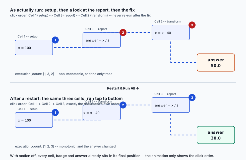
Here is a notebook that “works.” Three cells, run in this order by a real analyst building it: the first sets up a number, the third checks the answer, the second — added afterward, once a colleague pointed out the raw number needed a cleaning step — fixes it. The analyst never re-ran the third cell after adding the second. Nothing raised an error. Nothing looked wrong. The notebook was saved, and the number in the third cell’s output — the number that ended up in a slide the next day — was wrong.
This is not a contrived edge case. It is measured, on this machine, from a
notebook built and executed for real in this lesson’s lab. A clean top-to-bottom
run of the exact same three cells answers 30.0. Run in the order the analyst
actually clicked — setup, then a look at the report, then the fix, never
returning to the report — the same notebook, still open, still looking exactly
as it did a moment ago, answers 50.0. Here is both runs, verbatim from a real
execution:
Clean top-to-bottom run (order 0, 1, 2):
  execution_count: [1, 2, 3]
  cell 2 (report) final value: 30.0

Scrambled run (order 0, 2, 1 -- setup, then a look at the report, then the fix):
  execution_count: [1, 3, 2]
  cell 2 (report) final value: 50.0
Look at that output for a second time. Nothing distinguishes the two runs to a
reader scrolling past — both show a plain float in the last cell, no red text, no
warning banner. The only difference sits in a field almost nobody reads: the
scrambled run’s execution_count sequence, [1, 3, 2], is not sorted. The clean
run’s is. That is the entire evidence trail. If you have ever trusted a notebook
because it “already ran” and looked fine, you have trusted exactly the kind of
document this lesson is about.
The rule this day defends is short enough to say once and mean absolutely: restart and run all, or it did not happen. Not “it looks fine.” Not “I ran it yesterday and it worked.” A notebook’s claims are unverified — however carefully written, however plausible the numbers look — until it has survived a fresh kernel executing every cell, in document order, from nothing. Everything below this line is either a way that guarantee gets broken, or a way to check that it hasn’t been.
The idea in plain language
A notebook is two things wearing one file extension, and almost every notebook bug comes from forgetting they are different.
The first thing is the document: a saved list of cells, each with source
code, and — if it was run — whatever output that run produced, frozen in place.
The document is what you see when you open a .ipynb file. It is what gets
committed to version control, emailed to a colleague, and rendered by GitHub’s
preview.
The second thing is the kernel: a separate, running Python process that actually executes the code. The kernel has its own memory — its own namespace of every variable any cell has ever defined, in whatever order they were actually run. The kernel does not care what order the cells sit in the document. It does not care whether a cell that defined a variable still exists. It remembers exactly what happened to it, and nothing about what the document currently says.
A notebook “working” is a claim about the kernel’s history, not about the document’s content. Two notebooks with byte-identical cell source can behave completely differently depending on what has happened inside their kernels — and a notebook can look identical to a reader while recording two different histories, which is exactly what the opening example demonstrated. The rest of this lesson is variations on one move: hold the document still and change what the kernel remembers, or hold the kernel’s history still and change what the document shows, and watch the gap between them do the damage.
Historical background
The notebook interface traces to Mathematica’s notebook front end in the late
1980s, which paired a document of cells with an underlying evaluation kernel —
the same split this lesson is built around, decades before Python had one.
IPython added an interactive Python shell in 2001, and in 2011 the IPython
Notebook gave that shell a browser-based document with the now-familiar cell
structure. In 2014 the notebook’s language-agnostic parts split out from
IPython-the-language-specific-shell into Project Jupyter — the name itself an
allusion to Julia, Python and R, the three languages the new project meant to
serve equally through a shared protocol. The .ipynb file format,
nbformat, and the client/kernel messaging protocol that lets any language
implement a compatible kernel all date to this split.
The reproducibility problems this lesson covers were not new observations even
then. Out-of-order execution and hidden state are exactly the failure modes a
document/kernel split makes possible, and the community’s response has arrived
in layers over the following decade: nbconvert’s --execute flag to force a
clean re-run before converting; nbclient splitting out as its own execution
library so tools other than nbconvert could drive kernels programmatically;
nbstripout and similar pre-commit hooks once teams learned what committing
outputs did to their diffs; papermill, built at Netflix, for running
parameterised notebooks as scheduled jobs rather than by hand; and JupyterLab’s
own “Restart Kernel and Run All Cells” becoming the default advice given to
every new user precisely because so many bug reports turned out to be this
lesson’s opening failure in disguise.
What it is — and what it is not
A reproducible notebook is one whose displayed outputs are guaranteed to be what a fresh kernel, executing every cell in document order, would actually produce — nothing more, and the guarantee is binary: either the notebook has survived that exact test, or the claim is unverified.
It is not the same as a notebook that runs without error. The opening example ran without error and was still wrong. Absence of an exception proves only that the code the kernel actually executed didn’t raise — it says nothing about whether that execution matches what the document, read top to bottom, would produce.
It is not the same as a notebook with clean, well-commented code. Code quality and execution-order correctness are orthogonal; a beautifully written notebook can still have a report cell run before its data-cleaning cell.
It is not the same as a notebook that has been converted to a script and
that script running successfully. Converting a notebook to a .py file with
nbconvert extracts the cells’ source in document order — it does not
replay whatever order the kernel actually saw, and it does not tell you whether
the notebook’s saved outputs came from that order.
And it is not a property you can verify by reading. Nothing in a notebook’s
rendered view distinguishes a cell whose output came from a clean run from one
whose output came from a stale, out-of-order execution. The only artifact that
carries any trace at all is execution_count, and reading it requires knowing
to look — most readers do not.
Why it was created and what problems it solves
Interactive execution is the entire reason notebooks exist: run a cell, look at the result, adjust, run again, all without restarting the whole program. That workflow is what makes exploratory analysis fast. It is also, structurally, what makes reproducibility a problem rather than a given — every other artifact in this course (a script, a module, a pipeline) has exactly one way to run it, top to bottom, and a notebook’s whole value proposition is letting you run pieces of it in whatever order helps you think.
The problems that trade-off creates, all of which this lesson demonstrates for real rather than describing:
- Out-of-order execution silently changes answers, because a cell’s output is frozen at whenever it last ran, not recomputed when something upstream changes.
- Hidden state outlives its own cell, because deleting or editing a cell changes the document, not the kernel’s memory of what that cell already did.
- A notebook that “works” is not machine-checkable by inspection, because nothing in the rendered view distinguishes a stale output from a fresh one.
- Committed outputs make version control noisy, because a rerun of unchanged code still produces a different file, for reasons explored in detail below.
- Notebooks resist automated testing, because the natural unit of reuse in a notebook — a cell — is not something a test runner can import.
Every mechanism covered from here on exists to close one of these five gaps.
How it works
The notebook file is JSON
Strip away the rendered view and a .ipynb file is a JSON document with a
short, learnable shape: a list of cells, each carrying a cell_type
("code" or "markdown"), a source, and — for code cells that have been
run — an execution_count and a list of outputs. Here is a real cell, taken
verbatim from this lesson’s lab after executing 2 + 2 in a fresh kernel:
{
  "id": "2eb0881b",
  "cell_type": "code",
  "metadata": {
    "execution": {
      "iopub.status.busy": "2026-08-20T09:46:20.302857Z",
      "iopub.execute_input": "2026-08-20T09:46:20.303144Z",
      "shell.execute_reply": "2026-08-20T09:46:20.309351Z",
      "iopub.status.idle": "2026-08-20T09:46:20.310104Z"
    }
  },
  "execution_count": 1,
  "source": "2 + 2",
  "outputs": [
    {
      "output_type": "execute_result",
      "metadata": {},
      "data": { "text/plain": "4" },
      "execution_count": 1
    }
  ]
}
Every claim in this lesson is a claim about specific fields in this structure.
source is what the document says the code is. execution_count is what order
the kernel actually ran it in. outputs is what that run actually produced.
metadata.execution is a set of wall-clock timestamps the kernel’s execution
stamped on afterward — and it turns out to matter more than most tutorials
admit, in the section on output stripping below. Understanding this shape is
what makes every later section concrete rather than mysterious: this lesson’s
whole lab tests notebooks by building this exact JSON with nbformat,
executing it with nbclient, and asserting on these exact fields — no browser,
no click, ever involved.
Hidden state
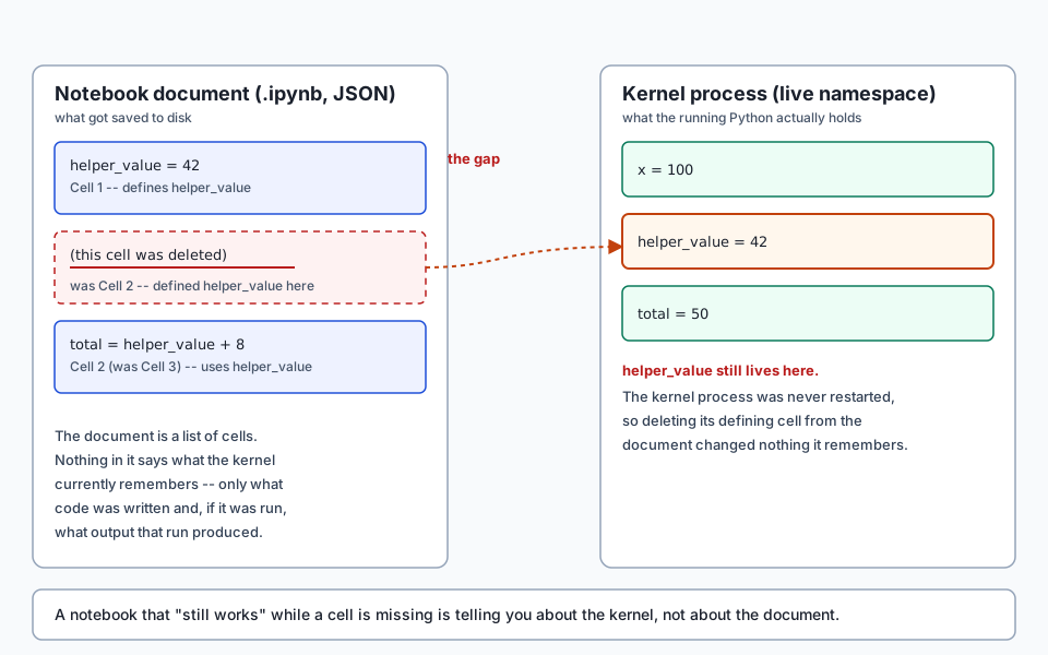
A variable defined in a cell that has since been deleted from the document does not stop existing. It stops existing in the document. The kernel process behind the notebook, if it has not been restarted, still holds it.
Measured directly: build two cells, one defining helper_value = 42, one
computing total = helper_value + 8. Run both in one kernel. Now delete the
first cell from the notebook — remove it from the document entirely, so the
saved file has exactly one cell, and that cell’s source has no mention of where
helper_value comes from. Rerun the remaining cell in the same kernel
process. It succeeds:
dirty kernel, cell A removed from doc, reran cell B: [{'output_type': 'execute_result', ...,
  'data': {'text/plain': '50'}, 'execution_count': 3}]
Now take that exact one-cell notebook — the one currently saved to disk, with no
trace of where helper_value comes from — and run it in a brand-new kernel that
has never seen any of this session’s history:
clean run raised CellExecutionError as expected
ename: NameError
Same file. Same cell. Two completely different outcomes, and the only variable is whether the kernel remembers a cell that no longer exists. This is not a rare accident; it is the single most common way “it works on my machine” happens with notebooks specifically — an analyst iterates, deletes what looks like dead scaffolding, and never notices the scaffolding’s side effect is still load bearing, because their own kernel has been open the whole time.
Out-of-order execution and what execution_count reveals
The opening example’s mechanics, stated precisely: nbclient lets you execute
individual cells against one persistent kernel in any order you choose, by
calling execute_cell on each cell index directly rather than calling execute
(which always proceeds top to bottom). Running cells [0, 2, 1] — setup, then
report, then the transform that was added afterward — stamps execution_count
values of 1, 3, 2 onto cells 0, 1, 2 respectively, because
execution_count records when a cell ran, not where it sits.
The diagnostic rule follows directly: a notebook run cleanly, top to bottom,
from a fresh kernel always produces a monotonically increasing
execution_count sequence — 1, 2, 3, ... — because each cell can only be
assigned a count once it has actually run, and a clean run visits them in
order. Any other sequence — gaps, repeats, or numbers out of position — is
direct, checkable evidence that the cells were executed in some order other than
the one the document displays them in. This is the only general-purpose signal
a reader has, short of re-running the notebook themselves, and it is why the
lab’s second exercise asserts on it directly: is_monotonic([1, 2, 3]) is
True; is_monotonic([1, 3, 2]) is False.
Restarting a kernel and running all cells always renumbers from 1, in
document order, regardless of what the counts were before — which is precisely
why “Restart & Run All” is the check that matters and reading execution_count
in a notebook someone else sent you is the check you actually have available
when you cannot run it yourself.
Execution as a test
Everything above becomes machine-checkable the moment you stop treating
“execute a notebook” as something that requires a person and a browser.
nbclient.NotebookClient(nb, kernel_name="python3").execute() runs every cell,
top to bottom, against a real kernel — headlessly, no display required — and
raises CellExecutionError the instant a cell errors, without touching any
cell after it.
Measured directly, executing a notebook whose second cell raises
ValueError('row_count below the expected minimum'):
ename ValueError evalue bad row countand the exception’s full message names the failing cell’s execution position
directly — Cell In[2], line 1 — and quotes the cell’s own source. That single
property is what turns “does this notebook still work?” from a question someone
has to remember to ask by hand into something a CI job can ask on every commit,
the same way pytest asks “do the tests still pass?” A broken notebook fails
the build with a message that already tells you which cell to look at, rather
than shipping and failing silently for whoever opens it next.
Outputs are committed, and what a rerun actually changes
Committing a notebook with its outputs means every rerun — even of completely
unchanged code — produces a different file, and folklore usually blames
execution_count. Measured directly, that turns out to be only sometimes true.
Two independent, fresh-kernel executions of 2 + 2 and 3 * 3, compared as
saved JSON:
unstripped identical? False
stripped identical? True
cell 0 field 'metadata' differs: {'execution': {'iopub.execute_input': '2026-08-20T09:46:43.654959Z', ...}}
  vs {'execution': {'iopub.execute_input': '2026-08-20T09:46:44.330183Z', ...}}
execution_count was identical between the two runs — both started counting at
1, because both were fresh kernels running deterministic code. What actually
differed was cell.metadata.execution: four ISO-8601 wall-clock timestamps
(iopub.status.busy, iopub.execute_input, shell.execute_reply,
iopub.status.idle) that nbclient stamps onto every cell on every execution.
Two runs a millisecond apart will never share those. Separately, this lesson
checked whether a plotted figure’s PNG bytes differ between runs of identical
plotting code — consistent with Day 133’s finding for matplotlib PNGs — and
found them byte-identical on this machine across two runs. So the actual,
measured source of “identical code, different commit diff” here is neither
image blobs nor execution_count; it is the per-execution timestamp metadata,
every single time.
An nbstripout-style pre-commit hook fixes this the direct way: strip
outputs, set execution_count to null, and delete
metadata.execution before every commit. Two runs of the same code then
produce byte-identical files. The trade-off is exactly as blunt as it sounds: a
stripped notebook reviews cleanly in a diff — no noise, no giant base64 image
blobs — but the committed file no longer shows what it produced. A reviewer
reading a stripped notebook is reading source code with no evidence attached;
they have to re-run it to see whether it still does what it claims. Whether
that trade is worth making depends on whether the repository is meant to be the
record of results (keep outputs, accept the diff noise) or purely the record of
method (strip them, and put results somewhere else — Day 133’s report is
exactly that somewhere else).
Parameterising a notebook
A parameterised notebook takes a single analysis and reruns it for several
inputs — one threshold, one date range, one customer segment per run —
without hand-editing the notebook each time. The mechanism, as papermill
documents and implements it, is specific: a cell tagged "parameters" (a tag
on the cell’s own metadata, not special syntax) holds the defaults, and running
a parameterised variant never edits that cell. Instead, a new cell tagged
"injected-parameters" is inserted immediately after it, carrying the run’s
actual values, so the original defaults stay visible in every executed output
notebook even though the run behaved according to the injected ones.
This lesson reproduces that exact mechanism by hand with nbformat — building
the tagged parameters cell, then building and inserting the injected cell —
because papermill itself is not installed in this lab’s environment and is
described from documentation only; no output attributed to papermill in this
lesson was produced by running it. Two variants built this way, threshold=10
and threshold=5, execute to different final filtered lists ([12, 15] versus
[12, 7, 15]) while every other cell’s source text — the default cell, the data
cell, the analysis cell — is character-for-character identical between the two.
That is the whole value proposition in one measured fact: the only thing that
changes between parameterised runs is the injected cell, which makes the
difference between two runs auditable by diffing exactly one cell.
Converting a notebook
nbconvert turns an already-executed notebook into another format by reading
its stored outputs — it does not, by default, re-execute anything (its
--execute flag does, and is the flag that forces a clean run before
conversion, closing the very gap this lesson opens with). Measured directly,
converting a two-cell notebook (one markdown cell of prose, one code cell
computing 40 + 74) to Markdown with nbconvert.MarkdownExporter:
## Row count check

We expect at least 100 rows after cleaning.


```python
row_count = 40 + 74
row_count
```


    114
Both the prose sentence and the computed value 114 — not retyped, taken
directly from the executed cell’s output — appear in the converted document.
That is the property that makes a converted notebook a usable report artifact
in Day 133’s sense: the document carries its own evidence rather than an
author’s transcription of it. nbconvert can equally target HTML for a
polished report or a .py script for a code review that does not want to open
a notebook viewer at all — the same source, the same executed outputs, three
different audiences.
The notebook/module split
Everything above assumes the notebook is where analysis lives, and that is only
correct up to a point. The moment logic is something other code depends on —
a cleaning function called from three different notebooks, a metric computed
the same way in an exploration notebook and a production pipeline — a notebook
cell is the wrong place for it to live, for a reason that is structural, not
stylistic: pytest can import and test a module directly, and cannot reach a
notebook cell at all.
Measured directly: calc.clean_mean, a small function living in an ordinary
.py module, is covered by an ordinary pytest test file — no kernel, no
notebook, nothing beyond a plain import. The identical averaging logic,
inlined into a one-cell notebook and executed inside a real kernel, computes the
right answer just fine — a kernel will happily run any code you put in front of
it. But asking Python’s own import system to reach that same logic by name —
importlib.import_module("clean_mean_inline_notebook") for a name that only
ever existed as text inside a cell — raises ModuleNotFoundError, every time,
regardless of whether a kernel is running. A .ipynb file is not something
Python’s import machinery understands; there is no special-casing that makes an
inlined function “count” as importable just because a kernel executed it once.
The rule this proves rather than merely states: exploration belongs in the notebook — trying things, looking at intermediate results, building the argument interactively. Anything downstream code needs to keep working belongs in a module with its own test suite, imported by the notebook rather than defined inside it. Day 126’s reproducible pipeline is exactly where that logic belongs once it graduates out of a cell.
Determinism inside a notebook
Day 126’s reproducibility manifest — seeds, pinned versions, a recorded environment — applies inside a notebook exactly as it applies to a script, and a notebook needs it more, not less, because interactive execution makes it easier to forget which environment produced a given output. A one-cell notebook that records its own environment, executed for real:
{'python_version': '3.14.0',
 'nbformat': '5.11.1',
 'nbclient': '0.11.0',
 'nbconvert': '7.17.1'}
The point of recording this is not decoration — it is a comparison target. A
stand-in for an older manifest, identical except nbformat pinned one minor
version back (5.10.0 instead of 5.11.1), disagrees with the live record at
exactly that key and no other, confirmed directly rather than assumed. A record
that cannot distinguish “the code changed” from “the environment changed” is
not doing its job; a record that changes precisely where a pin changed, and
nowhere else, is.
An everyday analogy
A notebook’s document is a recipe card pinned to the fridge. A notebook’s kernel is the pot actually on the stove. Reading the card tells you what steps were written down; it tells you nothing about what actually went into the pot, in what order, or whether someone added a pinch of salt straight from the shaker — a step never written on the card at all — before taking a photo of the finished dish. If a guest asks for the recipe and you hand them the card, they will follow the written steps and, if the pot’s actual history included something the card never mentioned, produce a different dish. The card looking complete and legible is not evidence the dish came from it. The only way to know the card actually reproduces the dish is to hand a stranger a clean pot, give them nothing but the card, and taste what comes out — which is exactly what “restart and run all” is: a clean pot, the card alone, and a taste test.
Examples in practice
The following table walks through this lesson’s own three-cell notebook —
setup sets x = 100; transform runs x = x - 40, added after the fact;
report computes answer = x / 2 — under four different execution histories,
each one executed for real in this lesson’s lab.
| Execution history | execution_count | Displayed answer | Trustworthy? |
|---|---|---|---|
Clean, top to bottom (0, 1, 2) | [1, 2, 3] | 30.0 | Yes — monotonic, matches document order |
Setup, report, transform (0, 2, 1) | [1, 3, 2] | 50.0 | No — non-monotonic; report predates the fix |
| Setup only, then transform, report never re-run | [1, 2, None] | (whatever report last showed) | No — report’s count did not advance at all |
| Restart & Run All, any prior history | [1, 2, 3] | 30.0 | Yes — the only history that always resets to this |
The second row is the opening failure. The third is a variant worth naming
separately: a cell whose execution_count never advanced this session at all is
displaying an output from some earlier session, possibly hours or days old —
None in that slot means “never run since the kernel currently attached to
this document started,” and a None sitting next to numbers is exactly as
diagnostic as a non-monotonic sequence.
For the hidden-state failure, the same treatment: a cell defining
helper_value = 42 is deleted from the document after a dependent cell has
already used it once.
| Where the notebook is run | helper_value’s defining cell in the document? | Result |
|---|---|---|
| Same kernel session, right after deletion | No | Succeeds — kernel still remembers it |
| Fresh kernel, notebook saved as-is | No | NameError, exactly as it should |
| Fresh kernel, defining cell restored | Yes | Succeeds — for the right reason this time |
The middle row is the version everyone eventually hits: a colleague, a CI job,
or the same analyst three weeks later opens the saved notebook, restarts the
kernel because that is the correct thing to do, and the notebook that “worked
fine” now fails on a NameError for a variable whose only definition is a cell
that no longer exists anywhere in the file.
Implications: security, privacy, performance, scalability, and cost
Security. A .ipynb file’s stored outputs can embed anything the executing
code produced — including, if the code printed one, a credential, a database
row, or an internal hostname. Committing outputs without reviewing them is a
credential-leak vector distinct from committing source code, because outputs
are data, not code, and code review habits do not automatically catch data
leaking through a printed repr(). A kernel itself, in this lesson’s lab and in
any local Jupyter setup, talks to its client over ZeroMQ on loopback
(127.0.0.1) only; nothing about running a notebook locally opens a port
reachable from outside the machine unless a hosted service is explicitly
configured to do so.
Privacy. The same stored-output risk applies directly to personal data: a
df.head() on a dataset containing names or identifiers, run once during
exploration and never cleared, sits in the committed file indefinitely, visible
to anyone with repository access, independent of any access control on the
original data source.
Performance. Kernel startup is the dominant fixed cost of executing a
notebook headlessly — on this machine, the first kernel start in a session
costs roughly one to two seconds; every cell execution after that is limited
only by the code itself. This matters for CI: executing many small notebooks
each in a fresh kernel pays that startup cost every time, and batching related
checks into fewer kernel sessions (which this lesson’s lab does throughout, via
client.setup_kernel() reused across multiple execute_cell calls) amortises
it.
Scalability. Parameterisation is the mechanism that scales a single
analysis notebook to many runs — one papermill invocation per parameter set,
each producing its own output notebook, rather than one person hand-editing and
re-running a shared file for each case, which does not scale past a handful of
variants before someone edits the wrong cell.
Cost. Every tool this lesson actually runs — nbformat, nbclient,
nbconvert, ipykernel, and locally-hosted JupyterLab itself — is free and
open source with no paid tier. The cost trade-offs in this space live entirely
in hosted execution: Google Colab’s free tier provides a shared, time-limited
kernel with no guarantee of GPU availability, while its paid tiers (Colab Pro
and Pro+) buy longer sessions, more reliable GPU access and more memory — costs
Colab’s own documentation states directly rather than figures reproduced here.
Alternatives: free, open source, and commercial
| Tool | When to choose it | How it is used | Free vs. paid | Run in this lesson? |
|---|---|---|---|---|
nbformat + nbclient + nbconvert | Testing or converting notebooks headlessly, from a script or CI, with no UI involved — exactly this lesson’s lab | nbformat.v4.new_notebook() to build; NotebookClient(nb).execute() to run; an nbconvert exporter to convert | Free, open source (BSD-3-Clause) | Yes — every output attributed to these three libraries in this lesson was produced by running them |
| JupyterLab | Interactive, exploratory work — writing and rerunning cells by hand, the ordinary day-to-day notebook interface | Launched with jupyter lab from the lab’s virtual environment; not something this lesson automates | Free, open source; hosted variants (e.g., a cloud JupyterHub) can carry infrastructure cost | No — described from documentation; no UI was driven for this lesson |
| Papermill | Running one notebook against many parameter sets as a batch or scheduled job, each producing its own output notebook | papermill input.ipynb output.ipynb -p threshold 5 from the command line, or its Python API | Free, open source | No — not installed in this lab; its parameter-injection mechanism is reproduced by hand with nbformat and described from documentation |
| Quarto | Publishing a notebook (or a plain .qmd document) as a polished report, book, slide deck or website, often mixing prose and code more heavily than a raw notebook | quarto render analysis.ipynb --to html, or authoring directly in .qmd with embedded code chunks | Free, open source (Quarto CLI); Posit Connect, a commercial product for publishing and scheduling Quarto content at scale, is paid | No — described from documentation only |
| Google Colab | Running notebooks with zero local setup, especially when GPU access is needed occasionally rather than constantly | Notebooks open directly in a browser against Google-hosted kernels; .ipynb files are otherwise standard and portable | Free tier: shared, time-limited kernels, GPU access not guaranteed. Colab Pro / Pro+: paid, longer sessions and more reliable GPU/memory, per Google’s own documentation | No — described from documentation only; no output in this lesson came from Colab |
nbstripout (and similar hooks) | Any team committing notebooks to version control that wants meaningful diffs rather than output-blob noise | Installed as a Git filter or pre-commit hook; strips outputs, execution_count and metadata.execution on every commit | Free, open source | Its effect (byte-identical stripped notebooks) is reproduced directly with a hand-written strip_outputs function, not the tool itself |
Comparison with related concepts
A notebook versus a script. A script has exactly one execution order: top
to bottom, every time, with no other option. A notebook’s entire value is
letting you choose a different order while exploring — which is also precisely
why a notebook needs an explicit reproducibility check a script does not:
running a .py file always tells you what a clean execution produces, because
there is no other kind.
Execution-as-a-test versus a unit test. A unit test asserts on a function’s
behaviour in isolation, independent of any notebook. nbclient executing a
notebook and raising on a failing cell is closer to an integration test: it
proves the whole document, cell order and all, still runs clean from nothing
— a check a unit test suite covering the same underlying functions cannot give
you, because the functions working correctly says nothing about whether the
notebook that calls them in a particular order still holds together.
Output stripping versus output retention. These are not “correct” and “incorrect” — they are two different answers to “what is this repository for?” Stripped notebooks are source code with clean diffs and no embedded evidence; notebooks with outputs retained are self-contained records with noisy diffs. Day 133’s separately-generated report exists precisely because neither answer is satisfying when the goal is “a document a non-technical reader can trust”: that report strips nothing and commits nothing incidental, because it is generated fresh from data and code every time, with its own provenance fingerprint rather than a notebook’s execution history.
Parameterisation versus a notebook with hardcoded values edited by hand. Both eventually produce the same set of output notebooks. The difference is auditability: a parameterised run changes exactly one cell (the injected parameters cell) and leaves everything else provably identical, which this lesson confirmed directly by comparing cell source text across variants. Hand editing a shared notebook for each run leaves no such guarantee — nothing stops an edit intended for one run from silently persisting into the next.
When to use it — and when not to
Restart-and-run-all discipline, execution-as-a-test, and an environment record are not optional extras for a “serious” notebook — they are what separates a notebook someone else can check from one they have to take on faith. Apply them whenever a notebook’s output will be read, cited, or acted on by anyone other than the person who just wrote it, including that same person a week later. That covers essentially every notebook that leaves a laptop: a shared analysis, a report, a model-training run, an AI experiment someone will try to reproduce.
The one place this discipline is legitimately relaxed is a notebook that is genuinely disposable — scratch exploration you will delete within the hour, never committed, never shown to anyone, existing purely to let you think. Even there, the moment a result from that scratch session is worth keeping, the right move is not to leave it in the scratch notebook; it is to restart, run clean, and only then treat the output as real — or, per the notebook/module split above, to move the logic that produced it into a tested module the moment anything else will depend on it.
Knowledge check
Eight questions covering execution order, execution_count, hidden state,
execution-as-a-test, output stripping, parameterisation and the notebook/module
split live in this lesson’s quiz.yml and render with the page.
Hands-on exercise
Build and run the lab in labs/sections/math-statistics-and-data/day-139-reproducible-notebooks/.
Nine exercises, all built with nbformat, all executed against real Jupyter
kernels through nbclient, none of them ever written to disk as a .ipynb
file:
- Prove out-of-order execution changes the answer.
- Prove
execution_countis non-monotonic exactly when order was scrambled. - Prove hidden state: a deleted cell’s variable survives in a dirty kernel and
raises
NameErrorthe moment the kernel is fresh. - Prove
nbclientfails a broken notebook and names the failing cell. - Prove exactly which JSON field makes two runs of identical code differ, and that stripping it makes them byte-identical.
- Build and execute two parameterised variants that differ only where they should.
- Convert an executed notebook to Markdown and prove the artifact carries its own prose and its own numbers.
- Prove a module’s logic is reachable by
pytestand an inlined cell’s is not. - Prove a notebook’s environment record changes when a pin changes.
cd labs/sections/math-statistics-and-data/day-139-reproducible-notebooks
python3 -m venv .venv
.venv/bin/pip install -r requirements/requirements.txt
.venv/bin/pytest starter -v
Expected output
A green run of the full harness ends:
7. Offline, and nothing left behind
  ok: no URLs inside examples/ or starter/ source
  ok: no .ipynb file anywhere inside the lab -- every notebook in this lab exists only in memory
  ok: no .ipynb_checkpoints directory anywhere inside the lab
  ok: no __pycache__ left behind (cleaned during this run)
  ok: no .pytest_cache left behind (cleaned during this run)

---------------------------------------------------------------
16 checks, 0 failure(s)
.venv/bin/pytest examples -q prints 12 passed; .venv/bin/pytest starter -q
prints 3 passed, 9 skipped before you begin the exercises.
Validate your work
Run bash tests/run_tests.sh from the lab directory and read its own exit
status directly — echo $? immediately afterward, with no pipe in between, so
nothing hides a real failure. 16 checks, 0 failure(s) and exit 0 is the
target. Then open expected-output/scrambled-vs-clean.txt and confirm for
yourself, by reading it, that 30.0 and 50.0 really are two different
answers from the same three cells with no error anywhere in either run.
Troubleshooting
Full detail lives in the lab’s troubleshooting.md. The two failures you are
most likely to hit: running pytest examples starter together, which aborts
collection with import file mismatch because both directories define
test_notebooks.py — always run them as two separate commands; and the
[IPKernelApp] WARNING | Kernel is running over TCP without encryption line
every kernel prints on startup, which is expected and harmless for a
loopback-only local kernel, not a failure.
Common mistakes
Building a fresh NotebookClient for every cell you want to execute is the
single most common way to accidentally erase the exact behaviour exercises 1
and 3 are testing — a fresh client starts a fresh kernel, so state that should
persist across cells (or should be absent) silently does the opposite of what
the exercise demonstrates. Use client.setup_kernel() as a context manager and
call execute_cell on it repeatedly, so one kernel process serves every call
inside that block.
Practice assignment
Take a notebook you have written for any earlier day in this course — or write
a short new one, three to five cells, doing any small piece of real analysis.
Using nb_lib.py from this lab as a starting point (or the raw nbformat /
nbclient calls it wraps), write a script that: executes your notebook cleanly
and records the final output of its last cell; executes it a second time in
some out-of-order sequence you choose by hand, picking an order that plausibly
mirrors how you actually built it; and prints both outputs side by side. If
your notebook’s answer does not change between the two runs, that is a real
and useful finding — say in one sentence why the particular cells you chose
happen not to be order-sensitive, rather than treating “no difference found” as
a failed exercise. Then add an environment-record cell to the notebook,
following this lesson’s environment_cell_notebook pattern, and confirm it
reports the actual versions installed in whatever environment you ran it in.
Extension challenge
Extend this lab’s exercise 5 (output stripping) to include a cell that produces
a matplotlib figure via %matplotlib inline and IPython.display.display,
executed twice independently. Confirm directly — do not assume — whether the
resulting image/png bytes are identical between the two runs on your machine,
the same way this lesson confirmed it for its own plotting check. If they are
identical, say so and explain that metadata.execution is still the only
field that differs, exactly as in the text-only version. If they are not
identical on your machine (a different matplotlib build, a different font
stack, and a different FreeType version can legitimately produce different
raster bytes from identical code, as Day 133 notes for the same reason), report
that too — a measurement that contradicts this lesson’s own finding on a
different machine is not a mistake in either lesson, it is exactly the kind of
machine-dependent fact expected-output/FIELDS.md exists to record honestly.
AI thread. Almost all substantive model work — trying a prompt, evaluating
an embedding, comparing two fine-tuning runs — starts life in a notebook,
because a notebook is the fastest way to look at one result and decide what to
try next. That is exactly the workflow this lesson shows is structurally prone
to producing an unverifiable claim: an experiment run interactively, cell by
cell, adjusted and re-run out of order as ideas change, whose final “the model
scored 0.91” can be exactly as stale as this lesson’s 50.0 — computed before a
later cell changed the data it depends on, displayed with no error, and cited
in a paper or a Slack message before anyone restarts the kernel to check. A
result a colleague cannot reproduce from a clean kernel is not a result; it is
an anecdote with a chart attached, and the gap between the two is not
effort or rigor in the abstract — it is one specific, checkable action:
restart, run all, and see if the number holds.
Quiz
Q1. A three-cell notebook is executed in the order setup, then report, then transform -- the report cell is never re-run after the transform. The notebook displays a plain number in the report cell with no error. What is the strongest true statement about that displayed number?
- It is definitely wrong, because out-of-order execution always produces an error
- It cannot be trusted without checking execution_count or re-running from a clean kernel, because it may have been computed before a later cell changed the value it depends on
- It is correct, because Jupyter always recomputes downstream cells automatically when an upstream cell changes
- It is correct as long as no cell was deleted
Show answer
Answer: B. It cannot be trusted without checking execution_count or re-running from a clean kernel, because it may have been computed before a later cell changed the value it depends on
Jupyter never recomputes downstream cells automatically -- that is exactly the gap this lesson exploits. A cell's displayed output is frozen at whatever it computed the last time it ran, regardless of what other cells did afterward. The measured example in this lesson executes cleanly (no error) and still displays 50.0 where a clean top-to-bottom run gives 30.0.
Q2. A notebook's execution_count sequence, read top to bottom, is [1, 3, 2]. What does that prove?
- Nothing -- execution_count is cosmetic and carries no information
- The notebook has an error somewhere
- The notebook was executed exactly twice
- The cells were executed in a different order than they appear in the document, specifically: cell 1 first, then the third-position cell, then the second-position cell
Show answer
Answer: D. The cells were executed in a different order than they appear in the document, specifically: cell 1 first, then the third-position cell, then the second-position cell
execution_count records the order the kernel actually processed each cell, not the order it happens to sit in the document. [1, 3, 2] means: first-position cell ran first, third-position cell ran second, second-position cell ran third -- a non-monotonic sequence is the one reliable signature of out-of-order execution, whether or not any cell raised an error.
Q3. A cell that defines `helper_value = 42` is deleted from a notebook. A remaining cell that uses `helper_value` still runs successfully. What does that tell you?
- The kernel process behind the notebook was never restarted, and its live namespace still holds helper_value even though no cell in the document defines it anymore
- Jupyter reconstructed the deleted cell automatically
- The remaining cell must not actually reference helper_value
- helper_value must be a built-in Python name
Show answer
Answer: A. The kernel process behind the notebook was never restarted, and its live namespace still holds helper_value even though no cell in the document defines it anymore
A kernel is a running Python process with its own persistent namespace. Deleting a cell only removes text from the document; it does not touch anything the kernel already executed. The same one-cell notebook run in a brand-new kernel raises NameError immediately, because the document, on its own, never defines helper_value.
Q4. Why does nbclient's execute() raising CellExecutionError on a broken notebook matter for CI, beyond just being able to detect an error?
- It does not matter -- any exception anywhere would do the same job
- It only matters for notebooks that produce plots
- It turns "does this notebook still work?" into a question a build pipeline can ask automatically, and the exception names the specific cell that failed rather than requiring someone to open the notebook and hunt
- It replaces the need to ever restart a kernel manually
Show answer
Answer: C. It turns "does this notebook still work?" into a question a build pipeline can ask automatically, and the exception names the specific cell that failed rather than requiring someone to open the notebook and hunt
Before execution-as-a-test, "does this notebook still work" required a person to open it, click Restart & Run All, and read every cell. nbclient does the same thing headlessly and, when a cell fails, raises an exception whose message names the cell's execution position and quotes its source -- exactly the information a CI log needs to point someone at the fix.
Q5. Two independent, fresh-kernel executions of the exact same notebook code are compared as committed JSON. Measured directly in this lesson's lab, what turned out to make them differ?
- The execution_count values, because every fresh run starts counting from a different number
- Nothing -- two runs of identical code always produce byte-identical notebooks
- The cell ids, which nbformat regenerates randomly on every execution
- Each cell's metadata.execution field -- four wall-clock timestamps nbclient stamps on every run -- while execution_count and the output data were identical between the two runs
Show answer
Answer: D. Each cell's metadata.execution field -- four wall-clock timestamps nbclient stamps on every run -- while execution_count and the output data were identical between the two runs
A common assumption is that execution_count is the noisy field. Measured directly: two fresh-kernel runs of the same deterministic code both start counting at 1, so execution_count matched exactly. What differed was cell.metadata.execution -- the iopub.status.busy, iopub.execute_input, shell.execute_reply and iopub.status.idle timestamps nbclient injects on every execution, which are wall-clock and therefore never identical between two runs.
Q6. An nbstripout-style hook strips outputs before every commit. What is the honest trade-off this lesson names for that practice?
- Stripping outputs makes a notebook execute faster
- A stripped notebook reviews cleanly in version control (no image-blob or metadata diffs), but it no longer shows its own results -- a reviewer has to re-run it to see what it actually produced
- There is no trade-off -- stripping outputs is strictly an improvement
- Stripping outputs is required before nbconvert can process a notebook
Show answer
Answer: B. A stripped notebook reviews cleanly in version control (no image-blob or metadata diffs), but it no longer shows its own results -- a reviewer has to re-run it to see what it actually produced
Committing outputs makes a notebook a self-contained record of what it produced, at the cost of noisy, often opaque diffs (image blobs, per-run metadata). Stripping outputs makes the diff meaningful again but turns the committed file into source code with no evidence attached -- a real trade-off, not a free improvement, and the right choice depends on whether the repository or a separate report is meant to carry the evidence.
Q7. In papermill's parameterisation model, what actually happens to a notebook's tagged "parameters" cell when a variant is run with different values?
- Every cell in the notebook is rewritten to hard-code the new values
- The parameters cell is deleted and replaced by a command-line argument
- The parameters cell is rewritten in place with the new values
- The parameters cell is left untouched, and a new cell tagged "injected-parameters" is inserted immediately after it, overriding the defaults for that run
Show answer
Answer: D. The parameters cell is left untouched, and a new cell tagged "injected-parameters" is inserted immediately after it, overriding the defaults for that run
Papermill never edits the tagged parameters cell -- it appends a new cell right after it carrying the run's actual values, which is why the original defaults stay visible in every executed variant even though the variant behaves according to the injected values. This lesson reproduces that exact mechanism by hand with nbformat, since papermill itself is not installed or run here.
Q8. Why, in this lesson's own account, does averaging logic belong in an imported module rather than staying inline in a notebook cell -- beyond general tidiness?
- Because nbconvert refuses to convert notebooks containing function definitions
- Because cells execute more slowly than module-level code
- Because notebooks cannot contain function definitions
- Because pytest can import and test a module directly, while a .ipynb cell is structurally unreachable by Python's import system -- importing a name that only ever existed inside a cell raises ModuleNotFoundError
Show answer
Answer: D. Because pytest can import and test a module directly, while a .ipynb cell is structurally unreachable by Python's import system -- importing a name that only ever existed inside a cell raises ModuleNotFoundError
The distinction proven directly in the lab: calc.clean_mean, defined in a module, is covered by an ordinary pytest test file with no kernel involved. The identical logic inlined into a notebook cell runs fine inside a kernel, but importlib.import_module raises ModuleNotFoundError for any name that only ever existed as text inside that cell -- pytest cannot reach it, with or without a kernel running.
Glossary
- Kernel
- The running process that actually executes a notebook's code. A kernel has its own persistent namespace -- every variable any cell has ever defined stays alive in it until the kernel is restarted or shut down, regardless of what the notebook document itself currently contains.
- execution_count
- The integer nbformat stores on every executed code cell, recording the order in which the kernel processed it -- not the order the cell sits in the document. A monotonically increasing sequence (1, 2, 3, ...) top to bottom is what a notebook run cleanly from a fresh kernel produces; any other sequence is direct evidence the cells were run out of document order.
- Hidden state
- A value a kernel remembers that no cell currently in the document defines. It arises when a cell that once defined a variable is deleted (or edited to remove that definition) without restarting the kernel, so cells that depend on the value keep working for whoever is still in that session and fail for anyone who opens the notebook fresh.
- Restart and run all
- The one operation that actually proves a notebook works: discard the current kernel, start a completely new one with an empty namespace, and execute every cell top to bottom in document order. Any claim a notebook makes without having survived this is unverified, however plausible its displayed outputs look.
- nbformat
- The Python library and JSON schema that define what a .ipynb file actually is: a list of cells, each with a source, a cell type, and -- for code cells -- an execution_count and a list of outputs. Building a notebook with nbformat produces the identical structure Jupyter itself would save.
- nbclient
- The library that executes a notebook against a real Jupyter kernel without opening any user interface. It is what nbconvert's --execute flag and Jupyter's own "Run All" ultimately call, and it is the library this lesson uses to turn "does this notebook still work" into an assertion a test suite can make.
- CellExecutionError
- The exception nbclient raises when a cell's execution fails during an nbclient run. It carries the original exception's name and message (.ename, .evalue) and names the failing cell's execution position in its string representation, which is what lets a CI log point directly at the broken cell.
- nbconvert
- The library and command-line tool that converts an executed notebook into another format: Markdown or HTML for a report, or a plain .py script for code review. Conversion reads the notebook's stored outputs; it does not re-execute cells unless told to with its own --execute flag.
- Output stripping
- Clearing a notebook's outputs, execution_count and per-cell execution timestamps before it is committed to version control, typically via an nbstripout-style pre-commit hook. It removes the noisy part of a notebook's diff at the cost of removing the evidence the notebook was ever actually run.
- Parameters cell
- A cell tagged "parameters" (by convention, in the cell's metadata) that holds a notebook's default inputs. A parameterisation tool such as papermill locates this cell and inserts a new "injected-parameters" cell immediately after it for each run, overriding the defaults without editing the original cell.
- Papermill
- A tool that executes a parameterised notebook from the command line or a script, producing one output notebook per set of parameter values. This lesson describes and reproduces its parameter-injection mechanism from documentation; papermill itself is not installed or run in this lesson's lab.
- Quarto
- A publishing system, successor to R Markdown, that renders notebooks and plain-text documents with embedded code into reports, books, slides and websites across multiple languages. Free and open source; described from documentation only in this lesson, not run.
- cell.metadata.execution
- The dictionary nbclient writes into a code cell's metadata on every execution, holding four wall-clock ISO-8601 timestamps (iopub.status.busy, iopub.execute_input, shell.execute_reply, iopub.status.idle). Measured directly in this lesson's lab, this field -- not execution_count -- is what makes two runs of identical, deterministic code differ as committed JSON.
- Notebook/module split
- The discipline of keeping exploration in a notebook's cells while moving any logic other code depends on into an imported, separately tested module. A notebook cell is structurally unreachable by Python's import system -- pytest can test a module directly and cannot reach a cell, with or without a kernel running.
- Environment record
- A cell (or a companion file) that captures the interpreter version and the exact versions of the packages a notebook depends on at the moment it ran -- Day 126's reproducibility manifest applied inside a notebook, so a reader can tell whether a changed answer came from changed code or a changed environment.
Sources and further reading
- nbformat: The Jupyter Notebook Format — Project Jupyter (accessed 2026-08-20)
- nbclient: A client library for executing notebooks — Project Jupyter (accessed 2026-08-20)
- nbconvert: Convert Notebooks to other formats — Project Jupyter (accessed 2026-08-20)
- Jupyter Documentation — Project Jupyter (accessed 2026-08-20)
- Quarto guide — Posit, PBC (accessed 2026-08-20)
Kept in this browser, no account needed. Your progress page turns the whole record into one link you can bookmark or open on another device.