Machine Learning › Machine Learning Fundamentals › Day 141
Day 141: What Machine Learning Is and Is Not
After this lesson you will be able to state what machine learning is in one sentence -- function approximation from examples -- and derive from that sentence every property that makes it useful and every property that makes it dangerous. You will fit a one-nearest-neighbour model to a dataset whose labels are coin flips and watch it score exactly 1.000 on the data it memorised and 0.518, which is chance, on data it has not seen, so that a training-set number never persuades you of anything again. You will construct a problem where an exact three-line rule scores 1.000 and the best of four trained models reaches only 0.9675, and learn to ask whether the rule exists before reaching for a model. You will make a model's accuracy fall from 0.948 to 0.4895 by moving the input region without changing the rule, and see why nothing in the model can notice. You will measure a nearest-neighbour regressor at 0.180 error inside its training range and 139.704 outside it, and understand that as a property to respect rather than a bug to fix. You will put a majority-class baseline of 0.900 next to a model scoring 0.821 and see a good-looking accuracy lose to a constant. You will compute an irreducible ceiling of 0.750 from a known label-noise rate and confirm that four different model families all sit at or below it. And you will end with a four-question decision function that tells you, before any code is written, when machine learning is the wrong tool entirely.
Hands-on lab for this lesson
Lab files on GitHub: https://github.com/ai-roadmap-365/ai-roadmap-365.github.io/tree/main/labs/sections/machine-learning/day-141-what-machine-learning-is-and-is
- Get the hands-on files. Clone the labs repository once (you can reuse this clone for every lesson). This works on macOS, Linux, and Windows (PowerShell or WSL):
git clone https://github.com/ai-roadmap-365/ai-roadmap-365.github.io.git cd ai-roadmap-365.github.io - Open this lesson's lab. Move into the directory for this specific day. Every lab lives at the same predictable path — section / subsection / week / day:
cd labs/sections/machine-learning/day-141-what-machine-learning-is-and-is - Read the lab guide. Open `README.md` in that directory. It lists the exact commands, what each does, the expected output, and how to check your work — read it before running anything.
- Run it and check your work. Follow the README's "How to run" section: run the example first to see the finished result, then complete the numbered exercises in `starter/`, then run the tests. The tests pass (exit 0) only when your work is correct.
bash tests/run_tests.sh # or the test command named in the lab README
You can also open the lab as a local page (works offline, shows the file tree and expected output).
Learning objectives
By the end of this lesson you will be able to:
- Define machine learning as function approximation from examples, and name its three ingredients: data, a model class and an objective
- Produce a perfect 1.000 training accuracy from a model that has learned nothing, and explain why that number is arithmetic rather than achievement
- Write a nearest-neighbour classifier from scratch in NumPy and state the one condition under which its training accuracy is not exactly 1.000
- Explain why performance on seen data is free and performance on unseen data is the entire product
- Judge when a hand-written rule beats a trained model, and apply that judgement before reaching for a model
- Name the i.i.d. assumption plainly and demonstrate an accuracy collapsing under a distribution shift the model was never told about
- Distinguish interpolation from extrapolation with measured error on both sides of a training range, and treat the difference as a property rather than a defect
- Compare any reported accuracy against a majority-class baseline, including the case where a good-looking model loses to a constant
- Compute an irreducible error ceiling from a known label-noise rate and explain why chasing the last few points is often chasing noise
- Separate machine learning from reasoning, understanding, causal inference and database lookup, with a concrete demonstration of each distinction
- Account honestly for the cost of a model -- labels, maintenance, monitoring and the ethical inheritance of its training data
- Apply a four-question decision function to decide whether machine learning is the right tool, and defend the order the questions are asked in
Prerequisites
- Day 137 -- features and leakage: target leakage, train/test contamination and the instinct that a result which looks too good is a bug report. This day supplies the measurements behind that instinct
- Day 136 -- the untouched confirmation set and the forking-paths problem, which is the same discipline applied before models existed
- Days 117-118 -- the standard error, and why a small margin measured on a small sample is noise
- Day 119 -- the observational caveat, which returns here as the reason a model is never an explanation
- Day 138 -- data ethics, bias and provenance, whose obligations attach to every model trained on that data
- Comfort with NumPy array indexing and pytest, and a working python3 (3.11 or newer) on your PATH; the lab builds its own virtual environment from requirements/requirements.txt
Why this matters
Here is a model that scores a perfect 1.000 and has learned nothing at all.
Two hundred rows, four features drawn from a normal distribution, and labels produced by a coin flip. There is no relationship of any kind between the features and the labels — none, by construction, because the labels were never made by looking at the features. Fit a one-nearest-neighbour classifier to it, ask it to predict the labels of the very rows it was trained on, and it gets every single one right:
1-NN training accuracy (hand-written)          1.0
1-NN test accuracy (1000 unseen rows)          0.518
1-NN training accuracy (scikit-learn)          1.0
1-NN test accuracy (scikit-learn)              0.518
Those four lines are captured from a real run in today’s lab. The training accuracy is not 0.99 and it is not “about 1”. It is exactly 1.000, on this machine and on yours, under any version of any library, for any seed and any dataset — because a one-nearest-neighbour model predicts a point by finding the closest stored point and copying its label, and a training point’s closest stored point is itself, at distance zero. Perfection is not an achievement here. It is arithmetic.
On a thousand rows the model has never seen, it scores 0.518. That is chance. Two labels, a coin flip, and the model is a coin.
This is the first day of your machine learning course, and it opens by destroying the number that every conversation about machine learning starts with, because that number is going to be quoted at you for the rest of your career. Someone will show you a slide that says 94 percent. Someone will publish a benchmark. A vendor will send a case study. In almost every one of those cases, the single most important question — what was that measured on, and had the model seen it? — will not be answered on the slide, and often has not been asked at all.
You are not starting from nothing. Day 137 taught you leakage: target leakage, train/test contamination, temporal leakage, and the instinct that a result which looks too good is a bug report rather than a triumph. Day 136 taught you the untouched confirmation set and the forking-paths problem. Days 117 and 118 taught you that a 0.3-point margin measured on 500 examples is noise wearing a number’s clothes. Today’s job is to put a name and a mechanism under all of that, and to say precisely what this subject is, so that everything you build in the next eight weeks rests on a definition rather than an atmosphere.
Here is the definition the whole course will lean on:
Machine learning is function approximation from examples.
Every useful and every dangerous property of the field follows from that one sentence. It works spectacularly on inputs that resemble what it was shown. It fails silently on inputs that do not. It does not understand, it does not reason, and it does not know why anything happens. It finds a function that scores well on data like its training data, and then it will answer any question you put to it, in exactly the same confident tone, whether or not it has any business answering at all.
The idea in plain language
Strip away the vocabulary and there are three ingredients and one activity.
The three ingredients.
- Data — examples of the thing you want computed. For supervised learning, that means pairs: an input, and the output you wish the program would produce for it.
- A model class — the family of functions you are willing to search through. Straight lines. Decision trees up to some depth. Nearest-neighbour lookups. Neural networks of a given shape. You never search “all possible functions”; you always pick a family first, and that choice is a decision you are responsible for.
- An objective — a way of scoring one candidate function against the examples, so that “better” means something specific.
The one activity: search the family for a member that scores well on the examples.
That is all. There is nothing else in the definition. No understanding, no model of the world, no reasoning, no goals, no intentions. A trained model is a function: it takes an input and returns an output. The training procedure is a search. The objective is a number you chose.
What makes the subject interesting — and what makes it hard — is that scoring well on the examples is not the goal. It is trivially easy. The lab’s first exercise achieves a perfect score on pure noise in six lines by storing the training set and looking things up in it. Any model with enough capacity can memorise; memorising is the cheapest thing a computer does.
The actual goal is generalisation: performing well on data the model has never seen, drawn from the same source as the data it was trained on. Performance on data you have already shown the model is free and means nothing. Performance on data you have not shown it is the entire product.
Hold those two sentences next to each other, because almost every mistake in this field is a failure to keep them apart:
| What you measured | What it costs to get | What it tells you |
|---|---|---|
| Accuracy on the training data | Nothing — it is free, and a big enough model can always make it perfect | Whether the model can memorise. It can. Every model can |
| Accuracy on data held out and never touched | A discipline you have to impose on yourself | An estimate of how it will behave on the next real input, if that input resembles what you trained on |
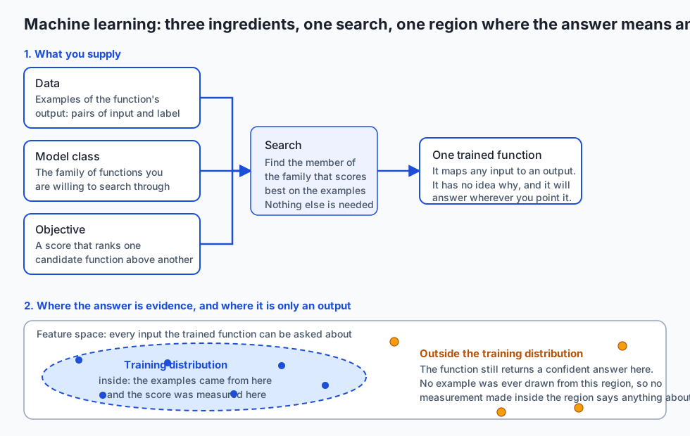
The diagram is worth a moment. Notice what is drawn as a region rather than as a word: the training distribution. “In distribution” and “out of distribution” are not adjectives describing a mood. They describe whether an input falls inside or outside the area your examples came from, and the whole value of a measured score is confined to the inside of that shape. The trained function does not know where the boundary is. It was never given one. Ask it about a point in the orange region and it will answer with exactly the same confidence it uses inside the blue one.
Historical background
The ideas here are older than the hardware, and the dates are worth knowing because they show how long the central problem has been understood.
1936 — the iris measurements. Ronald Fisher published “The use of multiple measurements in taxonomic problems” in the Annals of Eugenics, using flower measurements collected by the botanist Edgar Anderson: 150 specimens, three species, four measurements each. That dataset ships inside scikit-learn today and is the one you will use in the lab. It is nearly ninety years old and it is still a good teaching set for the same reason it was a good example then: it is small enough to look at and structured enough to be learnable.
1951 — nearest neighbours. Evelyn Fix and Joseph Hodges, working at the USAF School of Aviation Medicine at Randolph Field, Texas, produced the technical report that introduced nearest-neighbour classification. The rule was almost embarrassingly simple: to classify a new point, find the most similar known point and copy its answer. It is the model that opens today’s lab, and its simplicity is exactly what makes its perfect training score so obviously empty.
1957-1958 — the perceptron. Frank Rosenblatt, at the Cornell Aeronautical Laboratory in Buffalo, New York, built the perceptron and described it in Psychological Review in 1958 as “a probabilistic model for information storage and organization in the brain”. This was the first widely publicised system that adjusted its own parameters from examples, and it produced the first great cycle of overclaiming and disappointment in the field’s history — a cycle that has since repeated at roughly generational intervals.
1959 — the name. Arthur Samuel published “Some studies in machine learning using the game of checkers” in the IBM Journal of Research and Development. Samuel’s checkers program improved by playing, and his paper is where the term “machine learning” enters wide use.
1967 — the theory catches up with the trick. Thomas Cover and Peter Hart published “Nearest neighbor pattern classification” in the IEEE Transactions on Information Theory, proving results about how well the nearest-neighbour rule can do in the limit. This matters for today’s lesson because it is the moment the field started asking not “does this score well?” but “what is the best any method could possibly do here?” — which is the same question as today’s noise ceiling.
1971 onward — learning theory. Vladimir Vapnik and Alexey Chervonenkis developed the theory relating the capacity of a model class to the gap between its performance on training data and its performance on new data. The generalisation gap you will measure in the lab is not an anomaly discovered by practitioners; it is the central object of a mathematical theory that is now over fifty years old.
1997 — the definition most people quote. Tom Mitchell, in Machine Learning (McGraw-Hill), wrote the formulation you will meet everywhere: a program learns from experience E with respect to a task T and performance measure P if its performance at T, as measured by P, improves with E. It is a good definition and it is doing something specific — it forces you to name the task and the measure before you are allowed to claim learning happened. Notice how much of today’s lesson is already inside it: if you cannot say what P was measured on, you have not made a claim that Mitchell’s definition would accept.
2007-2011 — the library. scikit-learn began as a Google Summer of Code
project by David Cournapeau in 2007 and was released publicly in 2010 by a team
at INRIA in France; the reference paper, “Scikit-learn: Machine Learning in
Python”, appeared in the Journal of Machine Learning Research in 2011. Its
design decision that matters most for you is a boring one: every model has the
same three methods, fit, predict and score. That uniformity is why this
lesson can use six different models without teaching you six different APIs —
and why Day 146 can teach the API properly without having to re-teach the
ideas.
What it is — and what it is not
The denials matter more than the affirmations, because the affirmations are what marketing already tells you. Take each one seriously.
It is not reasoning. A trained model does not derive a conclusion from premises. It computes an output from an input by a fixed procedure that was selected because it scored well on some examples. The distinction is not philosophical hair-splitting; it is operational. A reasoning system that is given a new rule can apply it immediately. A trained model given a new rule can do nothing with it at all until someone produces examples of the rule being followed and runs the search again.
It is not understanding. The lab’s exercise 1 is the cleanest possible demonstration: a model scoring 1.000 on data with no structure whatsoever. Whatever “understanding” means, it cannot be something you can obtain in full measure from a table of coin flips. A high score is compatible with total absence of comprehension, and today you will produce that combination on purpose so you never mistake the one for the other again.
It is not causal inference. This is Day 119’s observational caveat coming back with a model attached. A model finds associations that predict the label in the training data. It does not, and structurally cannot, tell you what would happen if you intervened. If umbrella sales predict rain in your data, a model will happily use umbrella sales to predict rain, and it will be right, and banning umbrellas will not stop the weather. Every model is a prediction machine and no model is an explanation, no matter how much its feature importances look like one.
It is not a database lookup — except when it literally is. This is worth
sitting with. The one-nearest-neighbour model in today’s lab is a database
lookup: fit stores the training set and predict runs a nearest-match query
against it. That is why its training accuracy is exactly 1.000. Most models are
not lookups — a depth-3 decision tree throws away almost everything it saw and
keeps a few thresholds — but the extreme case is instructive, because it shows
what a training score measures at the limit: the model’s ability to retrieve,
not its ability to answer.
It is not a substitute for a rule you could write down. This is the single most useful piece of professional judgement in today’s lesson and it is rarely taught, so it gets its own section below and its own exercise in the lab. If the correct answer can be computed by a rule you can state, state the rule. A rule is exactly correct, costs nothing to run, requires no labels, cannot drift, and can be reviewed by a person who is not you. A trained model that merely approximates it is strictly worse in every one of those dimensions, and you will have built a data pipeline to get there.
It is not free, and it is not finished when it ships. A model is an asset that decays. It needs labels to be born and monitoring to stay alive. More on that in the implications section, because the cost is where most real projects actually fail.
So what is it? It is the best tool anyone has for problems where a correct answer exists, examples of it are available, and nobody can write the rule down. That is a genuinely large and genuinely important class of problems — reading handwriting, recognising speech, flagging anomalies, ranking documents, predicting demand — and for those problems nothing else comes close. The denials above are not an argument against the field. They are the shape of the tool, and knowing the shape is what lets you pick it up by the right end.
Why it was created and what problems it solves
Consider the task of reading a handwritten postcode.
You could try to write the rule. Take a scanned digit and write conditions: if the stroke closes into a loop with no tail, it is a zero; if there is a vertical line, it is a one. People genuinely tried this for years. It fails, and it fails in a specific way that is worth naming: not because the problem is impossible, but because the rule exists and no human can write it down. You recognise a handwritten 4 in a few tens of milliseconds and you cannot say what procedure you ran. The knowledge is real and it is inaccessible to introspection.
Machine learning is the answer to exactly that situation. It replaces “state the rule” with “supply examples of the rule being followed correctly, and let a search find a function that agrees with them”. You do not need to know the rule. You need to be able to recognise correct answers well enough to label a few thousand of them.
That reframing solves a specific and important class of problem:
- Perception — vision, speech, handwriting. The rule exists in human heads and cannot be extracted.
- Problems with too many interacting factors to enumerate — demand forecasting, credit risk, recommendation. A person could write a rule; they could not write the rule that weighs four hundred weak signals correctly.
- Problems where the rule changes faster than you can maintain it — spam filtering is the classic case. A hand-maintained rule list is a losing battle against an adversary; a model retrained weekly on fresh labels is not.
- Problems where the rule is not known to anyone yet — predicting which molecules bind to a target, for instance.
Notice what is not on that list: computing value-added tax, validating an email address against a specification, applying a published pricing table, deciding whether a number is even. Every one of those has a rule, the rule is written down somewhere in public, and any model you train to approximate it is a worse version of a thing you can already have exactly.
How it works
The three ingredients, precisely
Write the supervised learning setup down properly, in words rather than in notation, because the notation is Day 147’s job and the words are today’s.
There is some function you wish you had. Call it the target. It maps inputs to outputs — a scan of a digit to the digit, a customer record to whether they will renew, four flower measurements to a species. You do not have it. What you have is a sample of its behaviour: pairs of inputs with the outputs the target produced, possibly with some errors in the recorded outputs.
You choose a family of candidate functions. You choose a scoring rule. A search procedure returns the member of the family that scores best on your sample. That returned function is your model.
Everything a practitioner argues about is a choice among those three. Which family? Which score? How is the search done, and how long for? Nothing else is in the definition, and if you find yourself confused by a paper or a product, asking which of the three it is talking about will usually resolve it.
A model, from scratch, in eleven lines
Here is the entire one-nearest-neighbour classifier from today’s lab. This is not a simplified version for teaching. It is the real thing, and it is the model that produced the 1.000 at the top of this lesson:
class HandwrittenNearestNeighbour:
    def fit(self, X, y):
        self.X_ = np.asarray(X, dtype=float)
        self.y_ = np.asarray(y)
        return self

    def predict(self, X):
        X = np.asarray(X, dtype=float)
        diff = X[:, None, :] - self.X_[None, :, :]
        sq_dist = np.sum(diff * diff, axis=2)
        nearest = np.argmin(sq_dist, axis=1)
        return self.y_[nearest]
Read fit again. It stores the data. That is the whole training procedure —
there is no search, no objective, no parameter. Read predict: it computes the
squared distance from every query row to every stored row, takes the closest,
and copies its label.
Now the crucial line of reasoning. If a query row is one of the stored rows,
its distance to itself is zero, and zero is the smallest a squared distance can
be. So argmin selects the row itself and predict returns its own label.
Every time. For every dataset. Which is why:
1-NN training accuracy (hand-written)          1.0
1-NN training accuracy (scikit-learn)          1.0
Both the eleven-line version and scikit-learn’s KNeighborsClassifier(n_neighbors=1)
report exactly 1.000 on labels that are coin flips, and both report 0.518 on
unseen rows. The library is not doing anything cleverer; it is doing this,
faster, with more options.
There is exactly one way that perfect training score can fail, and today’s lab
measures it rather than glossing over it. If two training rows have identical
features but different labels, the tie can be broken toward the wrong one.
That is not hypothetical: the iris dataset contains exactly one duplicated
feature row, at positions 101 and 142, both reading (5.8, 2.7, 5.1, 1.9).
Both carry the same species, so on iris’s real labels a 1-NN still scores
exactly 1.000. Permute the labels and the same pair drops it to 149 out of 150.
The lab asserts the structural part — that the scrambled score falls below
1.000 — because that is the part that is guaranteed.
Generalisation is the product
The gap between the score on data the model has seen and the score on data it has not is called the generalisation gap, and its size is the single most informative number in an evaluation report. From the lab, two gaps measured with the same model type on the same day:
| Data | Training accuracy | Accuracy on unseen data | Gap |
|---|---|---|---|
| iris, full-depth decision tree | 1.000 | 0.960 | 0.040 |
| Constructed data with 20 percent of labels flipped, full-depth tree | 1.000 | 0.6535 | 0.3465 |
Identical training scores. One model is excellent and one is nearly useless, and the training score cannot tell them apart. Only the second number can.
And then the finding that this day exists to deliver. On that same noisy dataset, a much simpler model — a single straight boundary, fitted by logistic regression — scores 0.780 in training, well below the tree’s perfect 1.000, and 0.7655 on unseen data, well above the tree’s 0.6535.
The better training score belongs to the worse model.
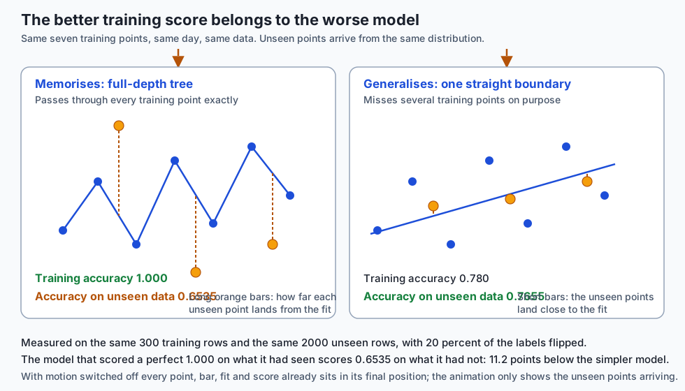
Why the simpler model wins here is Day 145’s subject and it will get a full treatment there. What belongs to today is the narrower and more permanent lesson: you cannot rank two models by their training scores. Not approximately, not as a rough guide, not “usually”. The ranking can be exactly backwards, and today you have a measured instance of it being exactly backwards.
The assumption nobody says out loud
Every claim a trained model makes rests on an assumption that is rarely written on the slide: that the data it will meet in future is drawn from the same distribution as the data it was trained on, and that each example is drawn independently. The shorthand is i.i.d. — independent and identically distributed.
It is a strong assumption and it is often false. Watch what happens when it breaks. In the lab, a decision tree is trained on points from the unit square labelled by a fixed rule. It is then tested twice: once on fresh points from the same square, and once on points from the identical problem translated three units away — same rule, same shape, different region.
in-distribution test accuracy                  0.948
shifted test accuracy                          0.4895
the rule, on the shifted region                1.0
The model scores 0.948 in distribution and 0.4895 — below chance — on the shifted region. Nothing about the model changed. Nothing about the underlying rule changed. The inputs moved, and the model has no way to notice, because nothing in its training data describes where the training data ended. It cannot raise a warning about a region it was never told exists.
That third line is the twist of the knife. The three-line rule scores 1.000 on the shifted region, because a rule is a statement about the world and a model is a statement about a sample.
Models interpolate; they do not extrapolate
A closely related property, and one that is regularly reported as a defect when
it is in fact the definition of the tool. Fit a nearest-neighbour regressor to
y = x² for x between 0 and 10, then measure its error inside that range and
outside it:
5-NN mean absolute error inside [0, 10]        0.18
5-NN mean absolute error outside, [10, 20]     139.704
5-NN largest prediction outside the range      97.307
largest target value ever seen in training     98.862
Inside the range the error is 0.180 — excellent. Outside it, 139.704, which is 774 times worse. And look at the third and fourth lines together, because they explain the mechanism entirely: the largest value the model predicts anywhere outside its training range is 97.307, and the largest value it ever saw in training is 98.862. It cannot predict a number bigger than one it has seen. Asked about x = 20, where the truth is 400, it returns the label of the closest thing it knows, which is somewhere near x = 10.
This is not a bug to be fixed. It is a property to be respected. A nearest-neighbour model is an interpolator by construction, and so, in the sense that matters, is every model: what a trained model does well is fill in between the examples. Fitting a straight line instead does not rescue you — the lab measures 6.007 error inside the range and 101.643 outside — it just fails in a different direction, because a line is not a parabola.
The baseline: the number you must beat before you have said anything
A score has no meaning without something to compare it against. The cheapest and most important comparison is the majority-class baseline: always predict the most common class, ignore the input entirely.
From the lab, a dataset where 90 percent of rows belong to one class and the features are pure noise:
majority-class baseline                        0.9
1-NN                                           0.821
full-depth tree                                0.817
Both trained models score about 82 percent. In a report, in a meeting, on a slide, “82 percent accurate” sounds like a working system. Both are worse than a constant that ignores the input. A model that cannot beat the majority class has demonstrated exactly nothing, and 82 percent looks nothing like nothing until you put the 0.900 next to it.
This is Day 117’s evaluation arithmetic applied. The same discipline that made you ask “compared to what, and with what standard error?” about an experimental result applies unchanged to a model score. And note the flip side, from the same lab exercise: on iris, where the features genuinely carry signal, the baseline is 0.260 and the 1-NN is 0.980. The comparison is what makes the second number impressive; without it, 0.980 is just a number that sounds high.
The ceiling you cannot climb over
Suppose you know that a fixed fraction of your labels are wrong — recorded in error, disputed between annotators, or genuinely ambiguous. Then there is a maximum accuracy no model can exceed on held-out data, and you can compute it before training anything.
In the lab, exactly 1000 of 4000 test labels are flipped — an exact count, not a probability, which makes the ceiling exact arithmetic rather than an estimate. A model that recovered the underlying rule perfectly would then be marked wrong on precisely those 1000 rows and score 0.750. Measured:
| Model | Accuracy on unseen data |
|---|---|
| The ceiling, 1 minus the noise rate | 0.750 |
| Logistic regression | 0.73725 |
| 15-nearest-neighbours | 0.72675 |
| Depth-3 decision tree | 0.68825 |
| Full-depth decision tree | 0.60875 |
The best model is 1.3 points below the ceiling. The remaining 26.3 points are not available to anyone — not to a bigger model, not to a better optimiser, not to a team with more budget. This is what makes the ceiling worth computing: it converts “we need to get from 0.737 to 0.95” from an ambitious target into a statement that is known in advance to be impossible, and it tells you that the remaining work is in the labels, not in the model.
It also explains why chasing the last few points is so often chasing noise. If you do not know your ceiling, every gap between your score and 1.000 looks like an engineering opportunity. Most of it is usually the data.
More data fixes one thing and not the other
“Get more data” is the field’s reflex answer, and it is right about half the time. The lab measures both halves.
| Problem | Small sample | Large sample | Gain |
|---|---|---|---|
| Variance-limited: a clean, intricate boundary | 0.5995 at n=50 | 0.99725 at n=5000 | 39.8 points |
| Noise-limited: a simple boundary, 30 percent of labels flipped | 0.6655 at n=200 | 0.68675 at n=5000 | 2.1 points |
A hundredfold increase in data takes the first problem from barely better than a coin to essentially solved: the boundary was always learnable, and the small sample simply did not reveal enough of it. Twenty-five times more data moves the second problem by 2.1 points against a ceiling of 0.700 that it was already within 3.5 points of at n=200.
Be honest about that 2.1: it is not zero. More data does help a little, because n=200 is genuinely a small sample and some of that gap was variance too. What more data cannot do is take a noise-limited problem past its ceiling, and the contrast — 39.8 points against 2.1 — is the shape of the decision. Before buying more labels, work out which of the two problems you have. The measurement that tells you is the ceiling, and the ceiling comes from re-labelling a sample and counting disagreements, not from training anything.
An everyday analogy
Think of a driver who has done the same commute every working day for six years.
They are astonishingly good at it. They know which lane clears first at the roundabout, which set of lights is badly timed on a Tuesday, where the road narrows without warning. Score them on that route and they are perfect: 1.000, every turn, no hesitation. That is the training accuracy at the top of this lesson, and it is real — they genuinely are excellent at this.
Now take them one street off the route. Not to another country; one street. The performance does not degrade gracefully in proportion to the distance. It falls off a cliff, because what they have is not a model of the city, it is a memorised sequence. That is the generalisation gap, and it is why the 1.000 told you nothing about how they would handle a diversion.
Close the road for resurfacing and the memorised sequence is not merely unhelpful, it is actively wrong: it confidently directs them into a barrier. That is distribution shift — the region moved, and nothing in six years of commuting contains any information about where the route stops applying. Our driver has no way to notice they have left it, which is exactly the model’s 0.4895 on the shifted region.
Drop them in a city they have never visited and ask for the fastest route to the station. They will produce an answer, confidently, based on the closest thing they know. That is extrapolation, and it is why the nearest-neighbour regressor’s largest prediction outside its range, 97.307, never exceeds the largest thing it saw, 98.862. You cannot return what you have never been given.
Two more turns of the same analogy, and then we will leave it alone.
Someone who has read the street map has something different in kind. They are slower on the commute — they will occasionally take a worse lane, scoring maybe 0.780 where the memoriser scores 1.000 — and they handle the diversion, the closure and the new district, because a map is a statement about the city and a memorised route is a statement about six years of Tuesdays. That is the simpler model beating the complex one on unseen data, and it is why the better training score belongs to the worse driver.
And finally: if the destination is signposted the whole way, nobody needs either. Follow the signs. They are exactly correct, they cost nothing, they do not need six years of commuting to produce, and they work in weather nobody has seen before. That is the rule, and choosing it over a model when it exists is the most professional decision in this lesson.
Examples in practice
If you can write the rule, write the rule
This deserves its own worked case because it is the one piece of judgement most courses skip.
Here is a problem with a genuinely exact rule. Two features, uniformly drawn. The label is 1 when the second feature exceeds the first, and 0 otherwise. Three lines:
def exact_rule(X):
    X = np.asarray(X, dtype=float)
    return (X[:, 1] > X[:, 0]).astype(int)
Now train some models on 300 examples and score everything on 2000 unseen rows:
| Approach | Accuracy on unseen data |
|---|---|
| The three-line rule | 1.000 |
| 15-nearest-neighbours | 0.9675 |
| Depth-8 decision tree | 0.9375 |
| Full-depth decision tree | 0.9375 |
| Depth-3 decision tree | 0.8855 |
Every model loses. Of course they do — they are approximating a function that is already written down, from a finite sample, using a family of shapes (axis-aligned splits, neighbourhoods) that cannot represent a diagonal exactly. The best of them is 3.25 points short and it needed 300 labelled examples, a training pipeline and a deployment story to get there. The rule needed none of those, is exactly correct on every input that will ever exist, and can be read and checked by a colleague in five seconds.
The professional error is not usually choosing the model over the rule knowingly. It is failing to ask whether the rule exists. In real systems the rule is often sitting in a regulation, a specification, a pricing table or a contract, and someone reaches for a model because modelling is the interesting part of the job. Ask first. Ask every time.
What the nine measurements say together
The lab measures nine claims. Read as a set, they say one thing nine ways.
| # | The measurement | What it is not telling you |
|---|---|---|
| 1 | 1-NN on coin-flip labels: train 1.000, test 0.518 | A training score is not evidence of anything |
| 2 | Rule 1.000, best model 0.9675 | A model is not always the right tool, even when it works |
| 3 | Train 1.000 both times; test 0.960 and 0.6535 | A training score cannot rank two models |
| 4 | 0.948 in distribution, 0.4895 shifted | A score is not portable outside the region it was measured in |
| 5 | Error 0.180 inside the range, 139.704 outside | A model is not a theory; it fills in between examples |
| 6 | Baseline 0.900, models 0.821 and 0.817 | A high-sounding accuracy is not necessarily better than a constant |
| 7 | Ceiling 0.750, best measured 0.73725 | A remaining gap is not necessarily an engineering opportunity |
| 8 | 39.8 points from more data, versus 2.1 | More data is not a general-purpose fix |
| 9 | Five distinct verdicts across six problems | ”Should we use machine learning?” is not a rhetorical question |
Implications: security, privacy, performance, scalability, and cost
Cost: the labels are the project. A model needs examples, and for supervised learning that means correct outputs, produced by someone who knows the answer. On any serious project the cost of obtaining, cleaning, arbitrating and re-checking labels dominates the cost of the modelling by a wide margin. Exercise 7’s noise ceiling is the reason this is not merely an accounting concern: label quality sets a hard bound on achievable accuracy, so under-investing in labels caps the project’s ceiling before anyone writes a line of modelling code.
Cost: a model is a liability that must be fed. Shipping a model is not the end of the work; it is the beginning of an obligation. The world moves, and exercise 4 is what “the world moved” looks like from inside the system: nothing errors, nothing alerts, accuracy simply becomes 0.4895 while the service keeps returning confident answers at the same rate. That failure mode is silent by construction, which means the monitoring has to be built deliberately — tracking the distribution of inputs, not just the error rate, because the error rate needs fresh labels and the input distribution does not.
Privacy: some models carry their training data inside them. The 1-NN in
this lesson stores its training set literally; fit is an assignment. If that
training set contains personal data, the model file is personal data, and
shipping the model ships the data. Most models are not this extreme, but the
general principle holds and is Day 138’s ethical inheritance in operational
form: the provenance and consent status of the training data attaches to
everything downstream of it, including a model artifact that looks like an
opaque binary.
Security: the input distribution is an attack surface. If accuracy collapses when inputs move outside the training region, then anyone who can influence your inputs can degrade your system without touching your infrastructure. They do not need an exploit; they need to send you unusual data. Systems whose inputs come from adversaries — spam, fraud, abuse — live permanently in this condition, which is why they are retrained on a schedule rather than trained once.
Performance and scalability. The two costs live in different places and it is worth knowing which is which. Training a nearest-neighbour model is instantaneous and predicting is slow, because every prediction compares against every stored row. Training a decision tree takes work and predicting is a handful of comparisons. Neither is “faster” in general; they move the cost. For a system serving predictions under a latency budget, the prediction cost is the one that will hurt you, and it is a property of the model class you chose on day one.
The honest accounting. Set against a hand-written rule, a model costs: labelled data, a training pipeline, a versioned artifact, a serving path, monitoring for input drift, a retraining cadence, a rollback plan, and a person who understands all of it. That is the correct comparison to make before choosing one, and it is why exercise 9’s first question is whether a rule exists.
Alternatives: free, open source, and commercial
Four options in this area, and the honesty note comes first: two of these were actually run to produce the numbers in this lesson, and two were not installed here and are described from their public documentation only, with no output reproduced.
scikit-learn 1.9.0 — run here
When to choose it. Classical machine learning on data that fits in memory, which covers a very large fraction of real problems. It is the default first choice for tabular data, and it is what this course uses through Course04.
How it is called. Every model exposes the same three methods, which is the library’s central design decision:
from sklearn.neighbors import KNeighborsClassifier

model = KNeighborsClassifier(n_neighbors=1)
model.fit(X_train, y_train)
predictions = model.predict(X_test)
Concrete example from this lesson. Everything measured today: the 1.000 and
0.518 in exercise 1, the 0.750 ceiling in exercise 7, the 0.900 baseline via
DummyClassifier in exercise 6. It also supplies the iris measurements
directly — load_iris reads a copy bundled inside the installed package, so no
download is needed.
Free or paid. Free and open source, BSD-3-Clause. No paid tier, no account, no usage limits. Day 146 teaches the API properly; today it is deliberately kept to one line per model.
NumPy 2.5.2, writing the model by hand — run here
When to choose it. When you need to know what a method actually does, when the method is simple enough to write in a dozen lines, and when a library’s behaviour has surprised you and you need a reference implementation to compare against.
How it is called. Directly, as arithmetic. The full model is the eleven lines shown earlier in this lesson.
Concrete example. The hand-written nearest-neighbour classifier reproduces scikit-learn’s numbers exactly — 1.000 and 0.518 on the same data — which is how today’s lab establishes that the perfect training score is a property of the method and not an artifact of a library.
Free or paid. Free and open source, BSD-3-Clause.
One caveat worth pinning down, because it will matter every time you claim a
result is reproducible: NumPy’s documentation states plainly that Generator
carries no version compatibility guarantee and that its bit stream may
change as better algorithms evolve. Seeding is therefore necessary and not
sufficient. Every number in today’s lab is reproducible given the seeds and
the pinned versions, and the lab’s expected-output/FIELDS.md separates the
four values that are exact everywhere by arithmetic from the twenty-one that
are exact only under those pins.
XGBoost — not installed here, described from its documentation
When to choose it. Gradient-boosted decision trees are the usual first choice for structured, tabular data where you want the strongest available accuracy rather than the simplest available explanation, particularly with mixed feature types and missing values.
How it is called. It offers a scikit-learn-compatible interface, so the call shape is the one you already know:
# Not run in this lesson: xgboost is not installed in this environment.
from xgboost import XGBClassifier

model = XGBClassifier(n_estimators=200, max_depth=4)
model.fit(X_train, y_train)
predictions = model.predict(X_test)
Concrete example. The natural use is exercise 7’s noise-limited problem: it would very likely land close to the same 0.750 ceiling as everything else, which is precisely the point — a stronger model class does not move a bound set by the labels. No output from XGBoost is reproduced anywhere in this lesson, because it is not installed in this environment and nothing here was run through it.
Free or paid. Free and open source, Apache-2.0 licensed. Commercially supported distributions exist from several vendors; the library itself has no paid tier.
A managed cloud AutoML service — not used here, described from documentation
When to choose it. When a competent tabular model is needed quickly by a team without a machine learning specialist, and the recurring cost of a managed service is preferable to the fixed cost of hiring for one. Services in this category — Google Cloud’s Vertex AI AutoML Tabular and Amazon SageMaker Autopilot are the two best known — take a labelled table, run model selection and tuning for you, and return a deployed endpoint.
How it is called. Typically not as a library at all: you upload a dataset,
name the target column, and receive an HTTP endpoint. The usage shape is a
request rather than a fit call, which changes where your data lives and who
can see it.
Concrete example. Nothing in this lesson was run through any managed service, no endpoint was created, and no vendor output is reproduced here.
Free or paid. Paid, and metered — typically by training time, by prediction volume, and by how long an endpoint stays deployed. This lesson does not quote any price, because published cloud pricing changes frequently and by region, and a figure that was not checked on the day you read it is worse than no figure. Check the vendor’s current pricing page before making any decision that depends on the number. What can be said without checking is structural: the recurring cost of a deployed endpoint continues whether or not anyone calls it, and the training data leaves your infrastructure — both of which belong in the comparison alongside accuracy.
| Option | Ran here | Best for | Cost |
|---|---|---|---|
| scikit-learn 1.9.0 | Yes — every number in this lesson | Classical ML on in-memory data | Free, BSD-3-Clause |
| NumPy 2.5.2, by hand | Yes — the eleven-line 1-NN | Understanding what a method does | Free, BSD-3-Clause |
| XGBoost | No — described from documentation | Strong accuracy on tabular data | Free, Apache-2.0 |
| Managed cloud AutoML | No — described from documentation | Speed without an in-house specialist | Paid, metered; no price quoted here |
Comparison with related concepts
Machine learning sits next to several neighbours that are regularly confused with it, and the confusions are expensive.
| Approach | What it produces | What it needs | Where it wins |
|---|---|---|---|
| A hand-written rule | An exactly correct answer | Someone who knows the rule | Whenever the rule can be stated. It is free, exact, reviewable and never drifts |
| Classical statistics | An estimate with an uncertainty attached, aimed at a question about a population | A model of how the data was generated, and assumptions you state | When you need to know how confident to be, and to defend it |
| Causal inference | An answer to “what would happen if we intervened” | A design — randomisation, or explicit causal assumptions | Whenever the decision is to change something, not to predict it |
| Machine learning | A function that predicts well on data like its training data | Labelled examples, and a distribution that holds still | When the rule exists but nobody can write it down |
| Mathematical optimisation | The best decision, given a fully specified objective and constraints | A specified objective and constraints | Scheduling, routing, allocation — when the model of the problem is known |
| A database lookup | The stored answer | The answer to have been stored | When the question has been asked and answered before, exactly |
Two of those distinctions deserve a sentence more.
Statistics and machine learning are not competitors; they answer different questions with overlapping mathematics. A statistician fitting a regression usually wants to say something defensible about a coefficient. A machine learning practitioner fitting the same regression usually wants the predictions to be good and does not care about the coefficient at all. You have spent Course03 building the first instinct, and it will make you unusually good at the second — because the habits that matter most here, holding out a confirmation set and asking what a margin means given the sample size, came from there.
Causal inference is the one to keep separate at all costs. A model’s feature importances look exactly like an explanation and are not one. Day 119’s observational caveat holds without modification: association measured in observed data does not license a claim about intervention, and adding a model on top does not change that.
When to use it — and when not to
Here is the checklist, in the order the questions should be asked. The order is the point: the cheapest disqualifying question comes first. Today’s lab implements this as a function and asserts its verdicts on six cases.
1. Can you write the rule down? If yes, write the rule. It is exactly correct, needs no labels, never drifts, costs nothing to run and can be reviewed by someone else. Verdict: write the rule.
2. Do you have labels — or can you get them? Supervised learning approximates a function from examples of its output. No examples, no approximation. Verdict: get labels first.
3. Will the distribution hold still long enough to matter? If the input distribution moves faster than you can retrain, the model is out of date before it ships. Verdict: not yet.
4. Can you tolerate being wrong sometimes? A model is an approximation and it will be wrong on some inputs. If a single wrong answer is unacceptable and cannot be caught downstream, an approximation is the wrong shape of tool regardless of its measured accuracy. Verdict: no.
If all four pass, use machine learning, and expect to keep paying for it.
def should_use_ml(problem):
    if problem["exact_rule_exists"]:
        return "write the rule"
    if not problem["labels_available"]:
        return "get labels first"
    if not problem["distribution_stable"]:
        return "not yet: the distribution moves"
    if not problem["errors_tolerable"]:
        return "no: errors are not tolerable"
    return "yes"
Applied to six real-shaped problems, from the lab:
| Problem | Verdict |
|---|---|
| Value-added tax at a published rate | write the rule |
| A rule exists, and nothing else does | write the rule |
| Sentiment of support tickets, none of them labelled | get labels first |
| Fraud in a payment network where adversaries adapt weekly | not yet: the distribution moves |
| An automated dosing decision with no human in the loop | no: errors are not tolerable |
| Handwritten postcode recognition | yes |
Notice the second row. A rule exists and there are no labels, no stability and no tolerance for error — and the verdict is still write the rule, because the rule does not need any of those things. That is what putting the cheapest question first buys you.
Knowledge check
Before the exercise, answer these from memory. If any of them is uncomfortable, re-read the section named beside it.
- Why is a 1-NN’s training accuracy exactly 1.000 rather than merely high, and what is the one condition under which it is not? (How it works)
- Two models both score 1.000 on their training data. What do you know about which is better? (Generalisation is the product)
- A colleague reports 82 percent accuracy on a classification task. What is the first question you ask? (The baseline)
- Your labels are 20 percent wrong. What is the highest accuracy any model can reach on similarly-labelled held-out data, and how do you know? (The ceiling)
- A model works in testing and degrades in production with no error and no alert. Name the assumption that broke. (The assumption nobody says out loud)
- When is the correct answer to “should we use machine learning here?” a flat no, even though labels exist and the distribution is stable? (When to use it)
The eight-question quiz for this day covers the same ground with the distractors that people actually pick.
Hands-on exercise
Today’s lab is labs/sections/machine-learning/day-141-what-machine-learning-is-and-is.
It has ten numbered exercises — the nine claims plus one measured exception —
in starter/test_ml_claims.py, each a pytest.skip naming the exact datasets,
helpers and values to assert. All the machinery lives in ml_lib.py and is
complete; the models are built by one-line helpers with their settings already
fixed, because today the models are not the subject.
Build the environment and see where you are starting from:
cd labs/sections/machine-learning/day-141-what-machine-learning-is-and-is
python3 -m venv .venv
.venv/bin/pip install -r requirements/requirements.txt
.venv/bin/pytest starter -q
Then work through the stubs one at a time, running pytest starter -q after
each. Print the measured pair in every exercise: a number you did not print is
a number you did not look at.
Run pytest starter and pytest examples as two separate commands. Both
directories contain modules with the same names, and a single
pytest starter examples invocation aborts collection with an
import file mismatch error — the harness checks that this is still true, so
you get to see the failure rather than take it on trust.
Expected output
Before you write anything:
3 passed, 10 skippedThe reference solution:
13 passedThe full harness:
13 checks, 0 failure(s)and echo $? prints 0. The measurement table, printed by
.venv/bin/python3 examples/report_measurements.py and captured verbatim in
expected-output/measured-values.txt, begins:
1. Perfect accuracy, zero learning (labels are coin flips)
  1-NN training accuracy (hand-written)          1.0
  1-NN test accuracy (1000 unseen rows)          0.518
  1-NN training accuracy (scikit-learn)          1.0
  1-NN test accuracy (scikit-learn)              0.518
  iris unique feature rows out of 150            149
  1-NN train accuracy, iris, scrambled labels    0.9933333333333333
Validate your work
.venv/bin/pytest examples -qreports13 passed..venv/bin/pytest starter -qreports3 passed, 10 skippedbefore you start and13 passedwhen you have finished all ten..venv/bin/python3 examples/report_measurements.pyprints a table byte-identical toexpected-output/measured-values.txt.bash tests/run_tests.shprints13 checks, 0 failure(s)and exits 0.- Break one assertion on purpose and confirm the harness reports it and exits
non-zero. This was done during authoring: changing
assert test_acc == 0.518to0.999produced13 checks, 2 failure(s)and exit 1, caught both by the pytest run and by the harness’s pytest-free reproduction of the same claims. Restore it afterwards.
Troubleshooting
No lab .venv found and the harness exits 2. It refuses to run against an
environment it cannot verify. Create it with the setup commands, or set
PYTHON and PYTEST to an interpreter that has the pinned versions — check 1
will tell you if it does not.
import file mismatch. You ran pytest starter examples in one
invocation. Run them separately.
ModuleNotFoundError: No module named 'ml_lib'. You ran pytest from inside
starter/ or from the repository root. Run it from the lab directory, naming
the directory.
A number differs in the last decimal place. Check pip list shows exactly
numpy 2.5.2 and scikit-learn 1.9.0. Every value here is deterministic given
those pins and the seeds in ml_lib.py; a different scikit-learn can break a
tie differently. expected-output/FIELDS.md says which values are
version-sensitive and which are exact everywhere.
test_01 fails with assert 1.0 == 0.518. You have swapped the training
and test sets. The perfect 1.000 belongs to the data the model memorised. This
is the mistake the whole day exists to prevent, so it is worth pausing on
rather than fixing quickly.
Common mistakes
- Reporting the training score. The most common mistake in the field, and it is committed by people who know better, because the training score is the one the fitting code has conveniently to hand.
- Comparing two models by their training scores. Exercise 3 measures the ranking coming out exactly backwards: 1.000 versus 0.780 in training, 0.6535 versus 0.7655 on unseen data.
- Quoting an accuracy without a baseline. 0.821 sounds like a result until the 0.900 baseline is next to it.
- Treating the gap to 1.000 as an engineering opportunity. Compute the ceiling first. In exercise 7, 25 of the missing 26.3 points are not available to anyone.
- Assuming more data will fix it. It fixes variance. It does not move a ceiling set by the labels: 39.8 points versus 2.1.
- Never asking whether a rule exists. Exercise 2’s rule beats every model and took three lines.
Practice assignment
Take a decision that is currently made by a model, a rule, or a person in something you use or work on — a spam filter, a recommendation slot, an eligibility check, an alerting threshold — and write a one-page evaluation brief for it, without training anything.
Answer these, in writing:
- What is the target function? State it as “input, output” in one sentence.
- Does an exact rule exist? Look properly: in a regulation, a specification, a pricing table, a contract. If one exists, stop and say so — that is a complete and valuable answer.
- What is the baseline? The majority class, or the current rule, or the status quo. Give a number if you can, and say how you would measure it if you cannot.
- What is the ceiling? How often would two competent people disagree about the correct label? That disagreement rate bounds the achievable accuracy, and estimating it costs a morning of re-labelling a sample rather than a quarter of modelling.
- What is the distribution, and how fast does it move? Name the specific thing that would have to change for accuracy to fall silently.
- What happens when it is wrong? Who notices, how soon, and what does it cost?
- Run
should_use_mlon it with honest answers, and write one paragraph on whether you agree with the verdict.
The deliverable is the brief, not a model. If your brief concludes “write the rule”, you have done the assignment correctly and saved more time than any model in this course will.
Extension challenge
Extend the lab’s exercise 7 in a direction it does not currently go: measure the ceiling on a dataset where you do not know the noise rate in advance.
Take iris, and corrupt an unknown-to-your-analysis fraction of the labels — have one function choose the rate from a seeded generator and hide it from the code that estimates it. Then estimate the ceiling without looking at that rate, using the disagreement between two independently corrupted copies of the same labels, and compare your estimate against the true value once you reveal it.
Report the estimate, the truth and the error honestly, including the case where your estimator is badly wrong — a small sample and a small label set make this genuinely hard, and a confident estimate from 150 rows deserves the standard error treatment of Days 117 and 118 rather than a decimal point. If your estimate turns out to be unusable at this sample size, that is the finding: write it down, say what sample size it would take, and you have learned something more durable than a number that happened to come out close.
AI thread. Every capability claim you will ever read about a modern model is a claim about a distribution, whether or not it says so. “It scores 89 percent on this benchmark” means: on inputs drawn from whatever process produced that benchmark, this system produced outputs a grader accepted 89 percent of the time. It says nothing about your inputs unless your inputs resemble those, and resemblance is not a feeling — it is the question of whether your data falls inside the orange region or the blue one in today’s first diagram. So you now have the one question that cuts through almost all of the marketing, and it is the same question in every case, from a tabular classifier to the largest system anyone has trained: what data does this resemble, and what happens when the input does not? The systems have become vastly more capable since Fix and Hodges wrote down the nearest-neighbour rule in 1951, and the honest answer to the second half of that question has not changed at all — the model will answer anyway, in exactly the same confident tone, and nothing in it knows that it has left the region where its score was measured.
Quiz
Q1. A one-nearest-neighbour model is fitted to 200 rows whose labels were generated by coin flips, with no relationship of any kind between the features and the labels. What is its accuracy on those same 200 rows, and why?
- Exactly 1.000, because every training point is its own nearest neighbour at distance zero, so predicting it returns its own stored label
- About 0.5, because the labels are random and randomness cannot be learned
- Somewhere between 0.7 and 0.9, depending on the seed and the number of features
- Undefined, because a model cannot be scored on data it was trained on
Show answer
Answer: A. Exactly 1.000, because every training point is its own nearest neighbour at distance zero, so predicting it returns its own stored label
This is arithmetic, not measurement. A 1-NN prediction finds the closest stored point and copies its label; for a training row the closest stored point is itself, at distance zero. The measured value in this lesson is exactly 1.0 for both the hand-written NumPy version and scikit-learn's, on labels that are coin flips. The 0.518 that option two is thinking of is the test accuracy on 1000 unseen rows, and keeping those two numbers apart is the whole point of the day.
Q2. Two models are trained on the same data. Model A scores 1.000 on the training set; model B scores 0.780. What do you know about which one will do better on new data?
- Model A, because a higher training score means a better fit to the underlying pattern
- Model B, because a lower training score always indicates better generalisation
- Nothing at all from these two numbers -- the ranking can be exactly backwards, and in this lesson it is
- Model A, provided both models come from the same family
Show answer
Answer: C. Nothing at all from these two numbers -- the ranking can be exactly backwards, and in this lesson it is
Measured in this lesson on the same noisy dataset: the full-depth tree scores 1.000 in training and 0.6535 on unseen data, while logistic regression scores 0.780 in training and 0.7655 on unseen data. The better training score belongs to the worse model. Option two overcorrects -- a lower training score does not always mean better generalisation either. Training scores simply do not rank models, and no amount of care in reading them changes that.
Q3. A classifier reports 82.1 percent accuracy on a held-out test set. Ninety percent of the rows in that test set belong to one class. What is the correct reading?
- A solid result -- 82 percent on held-out data is genuine evidence the model works
- Encouraging but incomplete; you would want a confusion matrix before concluding anything
- The model is well calibrated but poorly tuned, and needs a different threshold
- The model is worse than a constant that always predicts the majority class and ignores the input, which scores exactly 0.900
Show answer
Answer: D. The model is worse than a constant that always predicts the majority class and ignores the input, which scores exactly 0.900
This is the measured case in exercise 6: features that are pure noise, 90 percent of rows in one class, the majority-class baseline at exactly 0.900, a 1-NN at 0.821 and a full-depth tree at 0.817. Both trained models would be reported as "82 percent accurate" and both are worse than ignoring the input entirely. A confusion matrix is genuinely useful and comes later in this course, but you do not need one to disqualify this result -- one subtraction does it.
Q4. You know that exactly 25 percent of your labels are wrong, in training and in held-out data alike. What is the highest accuracy any model can reach on that held-out data?
- There is no fixed limit; a sufficiently large model can learn to correct the mislabelled rows
- About 0.750, because a model that recovered the underlying rule perfectly would still be marked wrong on the quarter of rows whose recorded labels are wrong
- 0.875, the midpoint between the noise rate and perfect accuracy
- It depends entirely on the model family; tree-based models are more robust to label noise
Show answer
Answer: B. About 0.750, because a model that recovered the underlying rule perfectly would still be marked wrong on the quarter of rows whose recorded labels are wrong
The ceiling is 1 minus the noise rate, and in this lesson it is exact rather than estimated because exactly 1000 of 4000 test labels were flipped. Four different model families were measured against it: logistic regression 0.73725, 15-NN 0.72675, a depth-3 tree 0.68825 and a full-depth tree 0.60875 -- all at or below 0.750. Computing the ceiling first is what stops you from spending a quarter on the 26.3 points that are not available to anyone.
Q5. A model trained on points from the unit square scores 0.948 on fresh points from that square and 0.4895 on the identical problem translated three units away -- same labelling rule, same shape, different region. Why does the model not raise a warning?
- It would, if the training code had enabled input validation
- Because the accuracy metric is inappropriate for shifted data and a different metric would show it
- Because nothing in its training data describes where the training data ended, so it has no way to represent the idea of being outside it
- Because the translation was too small; a larger shift would have triggered an out-of-range error
Show answer
Answer: C. Because nothing in its training data describes where the training data ended, so it has no way to represent the idea of being outside it
A trained model is a function from inputs to outputs. It was given examples, not a boundary, and there is no place inside it where the edge of the training distribution is recorded. That silence is the dangerous part: nothing errors, nothing alerts, and the service keeps returning confident answers at the same rate while accuracy sits below chance. Detecting this requires monitoring the distribution of inputs deliberately, which is a thing you build rather than a thing you get.
Q6. A 5-nearest-neighbour regressor is fitted to y = x squared for x between 0 and 10. Its mean absolute error is 0.180 inside that range and 139.704 on the range from 10 to 20. Its largest prediction anywhere outside the training range is 97.307, while the largest target it saw in training was 98.862. What do those last two numbers explain?
- That the model needs more training data at the upper end of its range
- That the mean absolute error is the wrong metric for extrapolation and a squared error would behave better
- That the model has a bug: a correctly implemented regressor would extrapolate the parabola
- That the model structurally cannot return a value larger than one it has seen, because a prediction is an average of stored neighbours -- extrapolation is not something it does badly, it is something it does not do
Show answer
Answer: D. That the model structurally cannot return a value larger than one it has seen, because a prediction is an average of stored neighbours -- extrapolation is not something it does badly, it is something it does not do
A nearest-neighbour prediction is an average over stored targets, so its output is bounded by the targets it stored. Asked about x = 20, where the truth is 400, it returns something near the edge of what it knows. This is a property to respect rather than a bug to fix -- and fitting a straight line instead does not rescue you: measured here, a linear model scores 6.007 error inside the range and 101.643 outside it, failing in a different direction because a line is not a parabola.
Q7. For a task where the label is exactly determined by a rule you can write in three lines, a depth-3 tree scores 0.8855, a depth-8 tree 0.9375 and a 15-NN 0.9675 on unseen data. The rule scores 1.000. What is the professional conclusion?
- Write the rule. It is exactly correct on every input, needs no labels, cannot drift, costs nothing to run and can be reviewed by someone else
- Use the 15-NN, since 0.9675 is close enough and a trained model will adapt if the rule ever changes
- Ensemble the rule and the 15-NN to get the best of both
- Collect more training data until a model matches the rule exactly
Show answer
Answer: A. Write the rule. It is exactly correct on every input, needs no labels, cannot drift, costs nothing to run and can be reviewed by someone else
The models are approximating a function that is already written down, from a finite sample, using shapes that cannot represent it exactly. Option four is the trap worth naming: more data narrows the gap and never closes it, and every extra example costs money to label. The genuinely common professional error is not choosing the model over the rule knowingly -- it is never asking whether the rule exists, because the rule is usually sitting in a specification or a regulation and modelling is the more interesting part of the job.
Q8. A problem has no rule anyone can write, no labelled examples at all, a stable distribution and full tolerance for occasional errors. What does the four-question decision function in this lesson return, and why is the order of the questions the point?
- "Yes", because three of the four conditions are satisfied and labels can be obtained later
- "Not yet: the distribution moves", because label scarcity and distribution instability are the same problem
- "Get labels first", because supervised learning approximates a function from examples of its output, and with no examples there is nothing to approximate
- "No: errors are not tolerable", because unlabelled data makes every prediction unverifiable
Show answer
Answer: C. "Get labels first", because supervised learning approximates a function from examples of its output, and with no examples there is nothing to approximate
The order runs: does an exact rule exist, are labels available, is the distribution stable, are errors tolerable -- cheapest disqualifier first. Here the first question passes and the second fails, so the verdict is "get labels first". The ordering earns its keep in a different case measured in the lab: a problem where a rule exists and there are no labels, no stability and no error tolerance still returns "write the rule", because a rule needs none of those things.
Glossary
- Machine learning
- Function approximation from examples. You choose a family of candidate functions and a way of scoring a candidate against your examples, and a search returns the member of the family that scores best. Nothing else is required for the definition -- in particular, no understanding, no reasoning and no model of the world.
- Model class
- The family of functions a training procedure is allowed to search through: straight lines, decision trees up to a given depth, nearest-neighbour lookups, neural networks of a given shape. You never search all possible functions; you always choose a family first, and that choice is yours to defend.
- Objective
- The score that ranks one candidate function above another during training, so that "better" means something specific. It is a number you chose, which is why a model optimises what you asked for rather than what you wanted.
- Generalisation
- Performance on data the model has never seen, drawn from the same source as its training data. It is the entire product of machine learning. Performance on data the model has already seen is free, can always be made perfect by a large enough model, and is evidence of nothing.
- Generalisation gap
- The difference between a model's score on its training data and its score on unseen data. Measured in this lesson at 0.040 for a full-depth tree on iris and 0.3465 for the same model type on data with 20 percent of labels flipped -- identical training scores of 1.000 in both cases, which is why the gap rather than the training score is the informative number.
- Majority-class baseline
- A predictor that ignores the input entirely and always answers with the most common class. It is the cheapest meaningful comparison for a classifier, and a model that cannot beat it has demonstrated nothing. Measured here at exactly 0.900 on a dataset where two trained models scored 0.821 and 0.817.
- Irreducible error ceiling
- The maximum accuracy any model can reach on held-out data, given a known fraction of wrong labels. If a fraction r of labels is wrong, a model that recovered the underlying rule perfectly would still be marked wrong on that fraction, so the ceiling is 1 minus r. Measured here as exactly 0.750 for a 25 percent noise rate, with the best of four model families reaching 0.73725.
- The i.i.d. assumption
- Short for independent and identically distributed: the assumption that future inputs are drawn from the same distribution as the training data, each drawn independently. Every claim a trained model makes rests on it, it is frequently false in production, and its failure is silent -- nothing errors and nothing alerts.
- Distribution shift
- What happens when the inputs a deployed model meets stop resembling the ones it was trained on. In this lesson a model scoring 0.948 in distribution scores 0.4895 -- below chance -- on the identical problem translated to a different region, while the underlying rule still scores 1.000 there.
- Interpolation and extrapolation
- Interpolation is filling in between the examples; extrapolation is answering beyond their range. Models interpolate. A nearest-neighbour regressor measured here has 0.180 error inside its training range and 139.704 outside it, and its largest prediction outside the range, 97.307, never exceeds the largest target it saw in training, 98.862 -- it structurally cannot return a value it has not seen.
- Label noise
- Recorded outputs that are wrong: mis-entered, disputed between annotators, or genuinely ambiguous. It is the usual cause of a low ceiling, it is measured by re-labelling a sample and counting disagreements, and it cannot be fixed by a better model or by more data.
- One-nearest-neighbour classifier
- A model whose fit step stores the training set and whose predict step returns the label of the closest stored point. Its training accuracy is exactly 1.000 by construction, because a training point's closest stored point is itself at distance zero -- unless two identical feature rows carry different labels, which is the sole exception and does occur in iris.
- Variance-limited versus noise-limited
- A problem is variance-limited when the boundary is learnable and the sample is too small to reveal it; more data helps decisively, measured here as a 39.8-point gain. It is noise-limited when the labels themselves are wrong; more data moves it barely, measured here as 2.1 points against a ceiling it already sat within 3.5 points of.
- Target function
- The function you wish you had, mapping inputs to correct outputs. You never have it. What you have is a sample of its behaviour, possibly with errors in the recorded outputs, and the model is your best approximation of it from that sample.
- The rule test
- The first question to ask of any candidate machine learning problem: can the correct answer be computed by a rule you can write down? If it can, write the rule. A rule is exactly correct, needs no labels, never drifts, costs nothing to run and can be reviewed by someone who is not you -- and in this lesson a three-line rule scores 1.000 where the best trained model reaches 0.9675.
Sources and further reading
- Getting Started with scikit-learn — scikit-learn developers (accessed 2026-08-24)
- Common pitfalls and recommended practices — scikit-learn developers (accessed 2026-08-24)
- Toy datasets, including the iris measurements — scikit-learn developers (accessed 2026-08-24)
- Random Generator -- NumPy reference — NumPy developers (accessed 2026-08-24)
- Machine Learning Basics -- Deep Learning, chapter 5 — Ian Goodfellow, Yoshua Bengio and Aaron Courville, MIT Press (accessed 2026-08-24)
Kept in this browser, no account needed. Your progress page turns the whole record into one link you can bookmark or open on another device.