Machine Learning › Machine Learning Fundamentals › Day 142
Day 142: Supervised, Unsupervised, and Reinforcement Learning
After this lesson you will classify a learning problem by the shape of its feedback signal rather than by its algorithm, and you will have measured why that distinction is the one that pays. You will produce two accuracy scores, 0.24 and 0.8933, for the identical clustering of the identical data, and understand that the 0.6533 between them came from cluster numbering alone. You will read a confusion table showing k-means isolating one iris species perfectly and blending the other two, and notice that you needed labels to find that out. You will watch standardising the features -- the advice in every clustering tutorial -- move the result measurably away from the species, from an adjusted Rand index of 0.7302 to 0.6201, and be able to explain the mechanism. You will see inertia fall at every value of k and understand why that is a theorem rather than a measurement, and watch a silhouette score confidently choose two clusters for a dataset with three species. You will build a ten-armed bandit and a tabular Q-learning agent from scratch in NumPy and measure that never exploring costs 0.3949 of optimal-action rate. You will count a terminal-only reward travelling backwards through a gridworld exactly one state per episode, and meet a one-line tie-breaking bug that makes the same agent reach the goal 0 times in 300 without raising a single warning. And you will find out why a clean, honest log of a working policy is not a supervised dataset -- five of eight greedy logs name the wrong action, four of them contain only one action, and even a well-explored log loses once to the winner's curse.
Hands-on lab for this lesson
Lab files on GitHub: https://github.com/ai-roadmap-365/ai-roadmap-365.github.io/tree/main/labs/sections/machine-learning/day-142-supervised-unsupervised-and-reinforcement-learning
- Get the hands-on files. Clone the labs repository once (you can reuse this clone for every lesson). This works on macOS, Linux, and Windows (PowerShell or WSL):
git clone https://github.com/ai-roadmap-365/ai-roadmap-365.github.io.git cd ai-roadmap-365.github.io - Open this lesson's lab. Move into the directory for this specific day. Every lab lives at the same predictable path — section / subsection / week / day:
cd labs/sections/machine-learning/day-142-supervised-unsupervised-and-reinforcement-learning - Read the lab guide. Open `README.md` in that directory. It lists the exact commands, what each does, the expected output, and how to check your work — read it before running anything.
- Run it and check your work. Follow the README's "How to run" section: run the example first to see the finished result, then complete the numbered exercises in `starter/`, then run the tests. The tests pass (exit 0) only when your work is correct.
bash tests/run_tests.sh # or the test command named in the lab README
You can also open the lab as a local page (works offline, shows the file tree and expected output).
Learning objectives
By the end of this lesson you will be able to:
- Classify a learning problem by its feedback signal -- instructive, absent, or evaluative -- rather than by the algorithm somebody used on it
- Apply the three diagnostic questions in the order that matters, asking whether your actions change your data before asking whether you have labels
- Demonstrate that cluster identifiers are arbitrary and that comparing them to class labels produces a number with no meaning
- Read a cluster-versus-class confusion table and state precisely what an unsupervised method did and did not recover
- Explain why inertia falls monotonically in k as a theorem, and why that makes it useless for choosing k
- Report a case where standard preprocessing advice measurably harms a clustering, and explain the mechanism
- Implement epsilon-greedy action-value learning from scratch and measure the price of pure exploitation
- Implement tabular Q-learning from scratch and count how far a terminal-only reward has propagated after n episodes
- Diagnose a silent reinforcement-learning failure caused by argmax tie-breaking on an all-zero value table
- Explain why logged policy data cannot be treated as a supervised dataset, in terms of what the log does not contain
- Recognise the winner's curse in an argmax over noisy estimates, and connect it to model selection
- Use unsupervised structure to spend a small label budget better, and quantify what choosing is worth
Prerequisites
- Day 141 -- machine learning as function approximation from examples, and why a training-set number persuades you of nothing. This day assumes you will not be impressed by an accuracy
- Days 117-118 -- the standard error and the sampling distribution, which is why today averages the bandit over 200 problems and the label-budget curve over 40 splits
- Day 136 -- the forking-paths problem, which returns today as the winner's curse in a different setting
- Day 119 -- randomisation and what an observational record cannot tell you, which is exactly the objection to training on a policy log
- Comfort with NumPy array indexing and reading a pytest failure, and a working python3 3.11 or newer on your PATH; the lab builds its own virtual environment from requirements/requirements.txt
Why this matters
Here are two accuracy scores for the same clustering of the same dataset:
accuracy taking cluster ids literally  : 0.2400
accuracy after the best relabelling    : 0.8933
difference, from numbering alone       : 0.6533
Nothing changed between those two lines. Not the data, not the algorithm, not the seed, not a single point’s group membership. The partition of the 150 iris flowers is byte for byte identical in both. What changed is which integer k-means happened to write on each group, and that integer is decided by where the algorithm’s centroids drifted during a numerical optimisation nobody inspected.
Sixty-five accuracy points, from a labelling convention.
That gap exists because the question “how accurate is this clustering?” is not a question. Clustering does not produce answers, so it cannot produce wrong ones. The moment you compare cluster identifiers to class labels you have smuggled in an answer key that the method was never given and does not know about — and if you are going to smuggle in an answer key, you may as well have used it properly in the first place.
This is the day the three-box diagram earns its keep or gets thrown away. You have seen it: supervised, unsupervised, reinforcement, three boxes with algorithms sorted into them. As a filing system for algorithms it is close to useless, because the same algorithm keeps turning up in more than one box. k-nearest-neighbours does classification and it does anomaly detection. A neural network does all three. Gradient descent does not care which box you are in.
The taxonomy that survives contact with real work is not about algorithms at all. It is about the shape of the feedback signal your learner is given — and once you see it that way, every practical consequence falls out of the shape rather than having to be memorised alongside it.
Three shapes, and only three:
| Setting | What you are told | What you are never told |
|---|---|---|
| Supervised | the correct output, for every input | nothing — you hold the answer key |
| Unsupervised | the inputs, and nothing else | whether anything you found is right |
| Reinforcement | how good the action you took was | what any other action would have paid |
The third row is the one that gets underestimated, and it is the one this lesson spends the most time on. Evaluative feedback is not weakened supervision. It is a categorically different kind of information, and the gap between the two is measurable. In today’s lab a reinforcement agent that never explores takes the best of ten actions 31.3% of the time. The identical algorithm, spending one pull in ten on a random action, takes it 70.8% of the time. Thirty-nine points, for a single parameter, because the greedy agent was never told what it was missing and never went to look.
The idea in plain language
Imagine three ways of being taught to cook.
In the first, you have a teacher standing beside you with the finished dish. Every time you produce something, the teacher shows you exactly what it should have looked like and tasted like. You can compare, adjust, and compare again. You will never be in doubt about whether you are improving, because the target is right there. This is supervised learning, and the reason it dominates practice is not that it is more powerful — it is that it is by far the easiest situation to be in.
In the second, you are handed a crate of ingredients and told to organise them. No recipes, no dishes, nobody to say whether you did it right. You could sort by colour, by weight, by shelf life, by cuisine, by which drawer they fit in. Every one of those is a real structure genuinely present in the crate. None of them is the structure, because there is no such thing. This is unsupervised learning, and its difficulty is not computational. It is that “correct” is undefined, and any evaluation you invent is a statement about your priorities rather than about the data.
In the third, you are cooking for a customer behind a hatch. You send out a dish, and some time later a number comes back: seven out of ten. You are not told what would have scored nine. You are not told which of your fifteen decisions cost you the three points. If you send out the same dish again you get another number, and if you never send out anything else you will never find out that the thing you stopped making in week one was the best dish on your menu. This is reinforcement learning, and its two distinctive difficulties are both visible in that description: the feedback is evaluative rather than instructive, and it is often delayed so far past the decision that connecting the two is itself the hard problem.
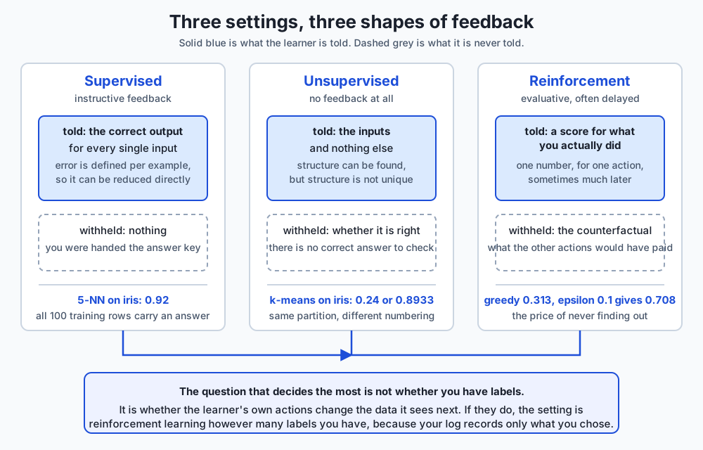
The single most useful thing on that diagram is the note at the bottom, and it is worth stating on its own because it contradicts the way the taxonomy is usually taught:
The deciding question is not whether you have labels. It is whether the learner’s own actions change the data it sees next.
If they do, you are in a reinforcement setting no matter how many labels you have, because your data is a record of what you chose and contains nothing at all about what you did not choose. Today’s lab measures exactly what that costs, and the number is worse than most people expect.
Historical background
The three settings arrived from three different intellectual traditions and were only retrofitted into one taxonomy afterwards, which is part of why the taxonomy fits so badly.
Supervised learning grew out of statistics and pattern recognition. Fisher’s 1936 paper introducing linear discriminant analysis — the paper that also introduced the iris measurements this lesson keeps using — is a supervised method in everything but name: it is handed labelled examples of three species and asked to find the combination of measurements that separates them. Rosenblatt’s perceptron in 1958 is the same setting with a learning rule attached, and the phrase “supervised learning” comes from that era’s habit of describing the label-provider as a teacher or supervisor.
Unsupervised learning came from a different direction: taxonomy and psychometrics, where the problem was never “predict this column” but “what groups are in here at all?” The k-means algorithm has a genuinely tangled lineage — Stuart Lloyd described the procedure at Bell Labs in 1957 in a paper about pulse-code modulation that was not published until 1982, while MacQueen’s 1967 paper gave it the name. Hierarchical clustering methods are older still and come out of biological classification. The field’s founding question was descriptive, not predictive, and that shows in its evaluation problem to this day.
Reinforcement learning came from psychology by way of control theory. Thorndike’s law of effect in 1898 — responses followed by satisfaction become more likely — is the whole idea in one sentence, sixty years before anyone could compute with it. Bellman’s dynamic programming in the 1950s supplied the mathematics of sequential decisions and, with it, the recursive value equation that everything since has been an approximation of. The modern field is usually dated to Sutton and Barto’s temporal-difference work in the 1980s and Watkins’ Q-learning in 1989 — the algorithm you will write out in full in today’s lab, in about thirty lines.
The names were tidied up later. Sutton and Barto’s textbook, first published in 1998, is largely responsible for the modern three-way framing, and it is also the source of the ten-armed bandit testbed that today’s lab reconstructs from scratch: ten actions, rewards drawn from Gaussians with different means, averaged over many independent problems because a single run is dominated by luck.
What the history explains is why the boundaries are messy. These are not three subdivisions of one field that were carved apart on principle. They are three separate research programmes that turned out to be doing related things, and the taxonomy is a retrofit.
What it is — and what it is not
Supervised learning is not “the one with a neural network” and unsupervised learning is not “the one where you do not know what you are doing”. Both are settings, defined by what information reaches the learner, and either can be attacked with almost any model family.
Here is what each is, stated precisely.
Supervised learning is function approximation from input-output pairs. You
are given examples (x, y) and asked to produce a function that maps new x
to a good y. The defining property is that the error on any training example
is computable — you have the target, so you can subtract. That single
property is what makes gradient descent, cross-validation, and every
evaluation habit from Day 141 possible.
Unsupervised learning is structure discovery from inputs alone. You are
given x and asked to say something useful about how it is arranged:
clusters, low-dimensional coordinates, density estimates, anomaly scores. The
defining property is that no target exists, so no error is computable, so
every evaluation is a proxy standing in for a judgement you have to make
yourself.
Reinforcement learning is learning a policy from evaluative feedback in a setting where your actions influence what you observe next. You are given a state, you choose an action, you receive a reward, and you land in a new state. The two defining properties are that the reward tells you about the action you took and nothing about the alternatives, and that your policy determines your data.
Now the things they are not, each with something today’s lab measures.
Unsupervised learning is not weakly supervised learning. It is not supervised learning with the labels temporarily mislaid. There is no hidden correct partition waiting to be recovered. When k-means splits iris into three groups, it has found a genuine structure — and the structure it finds is not the species. Here is what it actually did:
rows = species, columns = cluster id
  species 0: [0, 50, 0]
  species 1: [48, 0, 2]
  species 2: [14, 0, 36]
Species 0 is isolated perfectly: all fifty of its rows in one cluster, no other species in it. Species 1 and 2 are smeared across two clusters, with fourteen rows of species 2 landing in the cluster that is mostly species 1. That is a real and defensible partition of the measurements. It is simply not the species, because the species is not a property of the measurements — it is a property of the flowers, and two of these species overlap in petal and sepal space no matter how good your algorithm is.
Reinforcement learning is not supervised learning with a delay. This is the most consequential misconception in the lesson, and today’s lab attacks it directly. The intuition goes: surely, if I log everything my system does and the reward it got, I now have a labelled dataset and can train a supervised model on it. Let us test that. Eight independent ten-armed bandit problems, each played for two thousand steps by a purely greedy agent, every pull and every reward logged honestly. Then ask each log which arm was best:
greedy    logs: 3/8 name the truly best arm; 4/8 contain one arm only
epsilon=0.1 logs: 7/8 name the truly best arm; 0/8 contain one arm only
Five of the eight greedy logs are wrong, and four of them contain a single arm across all two thousand rows. There is no model, no amount of feature engineering, and no quantity of additional data that recovers what those logs do not contain. The rows about the other nine arms were never collected, because the policy never chose them. The data is not noisy; it is absent, and it is absent in a way that correlates exactly with what you want to know.
And supervised learning is not the default just because you have labels. The third row of that table is the one to sit with: a well-explored log still gets one of eight wrong, and the reason is instructive enough that the lab gives it its own exercise.
Why it was created and what problems it solves
Each setting exists because a class of problem genuinely does not fit the others, and the honest way to understand the taxonomy is to ask what breaks if you try to force a problem into the wrong box.
Supervised learning solves the problem of scale in judgement. A human can decide whether one email is spam. A human cannot decide it for a hundred million emails a day. If you can afford to have a human label a sample, a supervised model turns that finite judgement into an unlimited one. That is the entire commercial value proposition of the field, and it explains why supervised learning is the overwhelming majority of deployed machine learning: it is the setting where the business case is easiest to write down.
Unsupervised learning solves the problem of not knowing the question. Some of the time you genuinely do not have a target column and could not invent one. You have a million customer records and want to know whether there are natural groups. You have server logs and want to know what “normal” looks like so that you can flag what is not. You have three hundred features and want twenty coordinates that keep most of the information. None of those has a correct answer to supervise against, and inventing one would be dishonest.
It also solves a second, more practical problem: labels are the expensive part. Today’s lab measures this on iris with a 1-NN classifier and a label budget, averaged over forty splits because one split is not worth reading:
 3 random labels : 0.6455
 5 random labels : 0.7780
10 random labels : 0.8960
20 random labels : 0.9240
50 random labels : 0.9470
 3 chosen labels : 0.8760   (one per k-means cluster)
100 labels       : 0.9535   (every training row)
Three labels chosen by clustering the unlabelled data first and labelling one representative per cluster score 0.876. Three labels chosen at random score 0.6455. Same budget, twenty-three accuracy points apart, and the chosen three land between the five-random and ten-random figures — so, roughly, one well-chosen label is worth three careless ones here. That is unsupervised learning being used to make supervised learning affordable, which in practice is the most common reason to reach for it at all.
Reinforcement learning solves the problem of sequential decisions under consequences. Some problems are not “given this input, produce that output”. They are “given this situation, act — and live with where that puts you”. Game-playing is the obvious case. So is inventory management, so is recommendation when your recommendations shape what the user ever sees, and so is anything with a feedback loop between the model and its own future data.
The feedback loop is the whole story. In supervised learning your dataset is a fixed object that exists independently of your model. In reinforcement learning your dataset is generated by your policy, so a bad early policy produces data that confirms it. That is not an implementation detail. It is the reason exploration is a first-class concern rather than a tuning parameter.
How it works
The three ingredients of any feedback signal
Strip each setting to what actually reaches the learner and you get three questions with yes/no answers.
- Is there a target for this input? If yes, error is computable per example and you are supervised.
- Do the learner’s actions change what data arrives next? If yes, you are in a reinforcement setting regardless of the answer to question 1.
- Does feedback arrive at the moment of the decision, or later? If later, credit assignment becomes its own problem.
Today’s lab encodes exactly that in a function that refuses to guess:
def classify_problem(spec: dict) -> str:
    for key in ("has_labels", "actions_change_the_data", "feedback_is_immediate"):
        if key not in spec:
            raise KeyError(f"problem description is missing {key!r}")
    if spec["actions_change_the_data"]:
        if spec["feedback_is_immediate"]:
            return "reinforcement learning: contextual bandit"
        return "reinforcement learning: sequential, with delayed credit"
    if spec["has_labels"]:
        return "supervised learning"
    return "unsupervised learning"
The order matters, and it is the opposite of the order people usually reason in. Most engineers ask “do I have labels?” first. This function asks it last, because a problem where your actions change your data is a reinforcement problem even when every row is labelled — and treating it as supervised produces the failure the lab measures in exercise 8.
The KeyError is deliberate. A function that fills in a missing field with a
default is worse than one that refuses, because the guess is invisible in the
output and nobody reviewing the answer can see that it happened.
Unsupervised learning has no answer key, and every evaluation is a proxy
The clustering result from earlier is worth taking apart, because the way it misleads is the way every unsupervised evaluation misleads.
You cannot compute accuracy for a clustering. What people compute instead is one of these:
- An internal criterion — inertia, silhouette, Davies-Bouldin. These use only the data and the partition, so they are honest about not having labels, and they measure whatever geometric property they happen to encode rather than whatever you care about.
- An external criterion — adjusted Rand index, mutual information, best-permutation accuracy. These compare the partition to labels, which means they are not available in the setting they claim to evaluate.
Both are worth measuring, and the lab measures both. Start with the internal ones, at k from 2 to 6 on iris:
k=2: inertia  152.348   silhouette 0.6810
k=3: inertia   78.851   silhouette 0.5528
k=4: inertia   57.228   silhouette 0.4981
k=5: inertia   46.446   silhouette 0.4887
k=6: inertia   39.040   silhouette 0.3648
Two things there, and both matter more than the numbers.
Inertia falls at every single step, and it always will. This is a theorem
rather than a measurement: the best k-means objective at k+1 clusters can
never be worse than at k, because you can always take the k solution and
split one cluster to get a valid k+1 solution that is at least as good. So
“choose the k that minimises inertia” always answers k = n, one cluster per
point, on every dataset, forever. Any procedure built on inertia alone is
choosing k by where a human decided the curve had a bend.
Silhouette does choose, and it chooses two. Iris has three species. The silhouette score is not broken — at k=2 the partition genuinely is more cleanly separated, because species 0 sits well away from the other two while species 1 and 2 overlap. Silhouette is measuring separation, and separation is what it says it measures. It simply is not measuring “how many species are there”, because nothing in the data can measure that.
Structure is not unique, and the standard advice can lose
This one contradicts advice you will read in almost every clustering tutorial, and it was found by measurement rather than by argument.
The advice is: standardise your features before clustering, because k-means uses Euclidean distance and a feature measured in thousands will dominate one measured in tenths. That reasoning is correct and the advice is a good default. On iris it makes things worse:
ARI, raw clustering vs scaled          : 0.8036
ARI, raw clustering vs true species    : 0.7302
ARI, scaled clustering vs true species : 0.6201
Standardising moved the clustering measurably away from the species — adjusted Rand index 0.620 against 0.730 — while producing a partition that disagrees with the unscaled one on a fifth of its structure. The cause is not mysterious. Iris’s four features are all lengths in centimetres on comparable scales, so the problem standardisation exists to solve does not arise here. What standardisation does instead is equalise the features, which promotes sepal width — the noisiest and least discriminative of the four — to the same influence as petal length, which carries most of the separation.
The right conclusion is not “never standardise”. It is that preprocessing is part of the definition of the structure you are looking for, not a neutral preliminary. And notice the trap: you could only tell which was better by using the species labels, which the method does not have. In a real unsupervised problem you would be choosing between those two partitions with no way to check.
Evaluative feedback, and the measurable price of not exploring
Now the third setting. A ten-armed bandit is the smallest honest reinforcement problem: ten actions, each paying a reward drawn from a Gaussian with its own unknown mean, and a fixed number of pulls to spend. There are no states, so credit assignment does not arise yet. The only difficulty is the one that matters — you learn about an arm only by pulling it, and every pull spent learning is a pull not spent earning.
The whole agent is a dozen lines, and it is worth reading because everything about the setting is visible in it:
for t in range(steps):
    if chooser.random() < epsilon:
        arm = int(chooser.integers(k))        # explore
    else:
        arm = int(np.argmax(estimates))       # exploit
    reward = bandit.pull(arm)
    counts[arm] += 1
    estimates[arm] += (reward - estimates[arm]) / counts[arm]
That third-from-last line is the entire feedback signal: one number, for the one arm you chose. There is no vector. There is no counterfactual. The other nine arms had rewards on that pull too and you will never see them.
Averaged over two hundred independent problems of a thousand pulls each:
| epsilon | mean reward | fraction of pulls on the best arm |
|---|---|---|
| 0.0 (never explore) | 0.9838 | 0.3130 |
| 0.01 | 1.1314 | 0.4336 |
| 0.1 | 1.2800 | 0.7080 |
The greedy agent takes the best arm 31.3% of the time. Not because it is badly written — it is doing precisely what it was told, always taking the action with the highest current estimate. The problem is that its first few pulls fix those estimates, and an arm that got unlucky on its one and only pull is never tried again. It locks on, and it locks on to the wrong thing about seven times in ten.
Spending one pull in ten at random raises that to 70.8%, and raises mean reward by 30%. Thirty-nine points of optimal-action rate, bought with 10% of the budget, from a single parameter. This is what evaluative feedback costs you and why exploration is not optional. A supervised learner faces no version of this problem: it is handed every label whether it asked for the example or not.
Delayed feedback: credit assignment, made countable
The bandit had one state. Add states and the second difficulty appears.
Today’s gridworld is five by five. The agent starts top-left, the goal is bottom-right, moving costs nothing and reaching the goal pays one. The shortest path is eight steps. The interesting part is that the feedback for the first move arrives only after the eighth — and there is nothing in the world that tells the agent which of those eight moves earned the reward.
Q-learning solves this by bootstrapping: the value of where you land becomes part of the target for where you were.
target = reward + (0.0 if done else gamma * float(np.max(Q[s_next])))
Q[s, a] += alpha * (target - Q[s, a])
That is the whole algorithm. What it does is easier to see counted than described. Here is how many of the twenty-five squares carry a non-zero value after n episodes:
after   1 episodes:  1/25 states valued, greedy policy cannot reach goal
after   2 episodes:  2/25 states valued, greedy policy cannot reach goal
after   3 episodes:  3/25 states valued, greedy policy cannot reach goal
after   5 episodes:  5/25 states valued, greedy policy cannot reach goal
after  10 episodes: 10/25 states valued, greedy policy cannot reach goal
after  25 episodes: 18/25 states valued, greedy policy 8 steps
after  50 episodes: 20/25 states valued, greedy policy 8 steps
after 100 episodes: 21/25 states valued, greedy policy 8 steps
after 300 episodes: 22/25 states valued, greedy policy 8 steps
Exactly one new square per episode for the first ten. The reward walks backwards from the goal, one square per pass, because that is the only route information has: the square next to the goal learns from the goal, and the square before it learns from that square, and nothing can skip ahead.
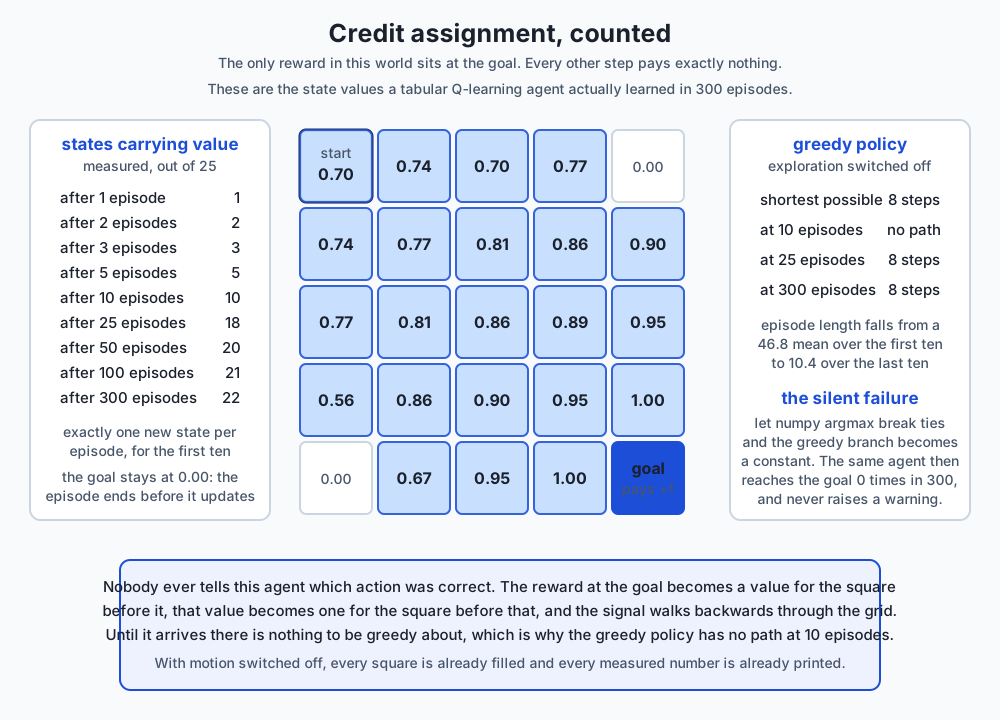
Three squares stay at zero even after three hundred episodes, and one of them is the goal itself. That is correct rather than broken: the episode terminates when the agent arrives, so the goal state’s own action-values are never updated. The other two are opposite corners the agent had no reason to route through. A value function is a record of where the agent has been and what it found there, not a map of the world.
The line worth carrying away is the middle column. Until episode 25, the greedy policy cannot reach the goal at all, because the value signal has not yet arrived where the agent starts. There is nothing to be greedy about. An engineer watching a flat learning curve at episode 10 and concluding the algorithm does not work would be wrong, and would be wrong in a way that no error message reports.
The bug that stops an agent learning without saying anything
While building this lab, the gridworld agent reached the goal in zero of three hundred episodes. No exception, no warning, no NaN. Just a flat line.
The cause is one function call:
a = int(np.argmax(Q[s]))np.argmax returns the lowest index attaining the maximum. That is
documented and correct. But a Q-table initialised to zeros makes every row one
enormous tie, so the greedy branch of an epsilon-greedy policy always returns
index 0 — which in this action table is “up”. With epsilon at 0.2, the agent
takes a random walk with a heavy upward bias, never leaves the top two rows of
the grid, times out at two hundred steps, and learns nothing because it never
finds the only reward in the world.
Fixing it is four lines:
def argmax_random_tiebreak(values, rng) -> int:
    values = np.asarray(values)
    best = np.flatnonzero(values == values.max())
    return int(best[rng.integers(len(best))])
And the contrast is total:
| Tie-breaking | Goal reached | Episode length, first 10 | Episode length, last 10 | Greedy path |
|---|---|---|---|---|
np.argmax | 0 of 300 | 200.0 | 200.0 | never arrives |
| random among ties | 300 of 300 | 46.8 | 10.4 | 8 steps |
Both configurations are in the lab, behind a flag, and both are asserted. The failure is more instructive than the fix, because it is representative: reinforcement learning bugs mostly present as nothing happening, and “nothing happening” is also what a correct agent looks like early on. The only defence is to instrument the thing that would distinguish them — here, whether the agent ever reached the goal at all.
Why a log of a working policy is not a supervised dataset
Return to the misconception, now with the mechanism visible.
An epsilon-greedy agent plays a ten-armed bandit for two thousand steps and logs every pull honestly. Here is the log:
seed 0, epsilon=0.1: best arm is 6, pulled 1813 of 2000 times
the other nine arms share 187 pulls
That imbalance is not a flaw in the logging. It is what a good policy produces — it found arm 6 and exploited it, which is its job. But now consider what the log is as a dataset: 90% of it is about one arm, and the nine alternatives share fewer than two hundred rows between them, at most thirty each. Any model trained on it inherits that. It will be confident about arm 6 and know almost nothing about the rest, which is exactly the wrong shape of knowledge for deciding whether something else would have been better.
With a greedy logging policy it gets worse: four of eight logs contain a single arm, and five of eight name the wrong arm as best. There is no statistical technique that fixes this, because the missing information was never recorded.
And then the case that is most worth understanding — the one log with full exploration that still gets it wrong:
| Arm | True mean | Logged mean | Pulls |
|---|---|---|---|
| 4 (truly best) | +0.9054 | +0.8634 | 1524 |
| 1 | +0.8216 | +0.9262 | 274 |
Arm 4 is genuinely better. It was pulled five and a half times as often. Its estimate is far more reliable — and that is exactly why it lost. With 1524 samples, arm 4’s estimate sits close to its true mean, slightly under. With 274 samples, arm 1’s estimate is free to wander, and it wandered up. Taking an argmax over noisy estimates does not pick the best arm; it picks whichever estimate is most inflated, and the noisiest estimates have the most room to inflate.
This is the winner’s curse, and it is not a bandit curiosity. You will meet it again on Day 144 under the name model-selection bias, where the thing being argmaxed is a set of validation scores instead of a set of arm means, and the consequence is that your chosen model’s validation score is systematically optimistic. Same mechanism, different clothes.
An everyday analogy
A restaurant reviewer, a shelf-stacker, and a gambler walk into the same supermarket.
The reviewer has a clipboard with the correct verdict for every product already written on it — supplied by a panel of experts who tasted everything last month. Their job is to learn to predict the panel’s verdict from the label on the jar. Every time they guess, they can turn the page and see the answer. If they get better at it, they will know immediately, and precisely by how much. This is supervised learning, and note what makes it tractable: the answer key exists, it is complete, and consulting it is free.
The shelf-stacker has no clipboard. Their job is to arrange four thousand products into aisles. They could group by category, by supplier, by price point, by how often things are bought together, by which shelf height fits the packaging. Every one of those produces a coherent supermarket. There is no panel to consult, and if the store manager says “aisle three feels wrong”, that is a preference, not a correction. This is unsupervised learning, and its difficulty is not that the job is hard. It is that “right” is a decision somebody has to make and then own.
The gambler is playing a row of slot machines. They pull a lever and money comes out, or does not. Nobody tells them what the machine next door would have paid on that pull. If they find one machine that pays and stay there all evening, they will go home believing it was the best machine in the row, with two thousand data points supporting them and no way to know they are wrong. This is reinforcement learning, and the two hard parts are both in that sentence: the feedback evaluates only what they did, and their own choices determined what they got to see.
The analogy earns its keep at one specific point. Ask what happens if the gambler writes everything down carefully and hands their notebook to the reviewer. The reviewer now has a clipboard of sorts — two thousand rows, honestly recorded, machine and payout. And the reviewer’s conclusion will be confidently wrong, because the notebook is a record of one gambler’s evening, and the machines they avoided are simply not in it. That is the whole content of “a log is not a supervised dataset”, and it is why the lab spends three exercises on it.
Examples in practice
Supervised, and correctly so
Spam filtering, credit scoring, medical image triage, demand forecasting, speech-to-text. What these share is not a domain — it is that a target exists, somebody can produce it for a sample, and the act of predicting does not change the thing being predicted.
That last clause is where the diagnosis actually happens. Demand forecasting in a warehouse is supervised. Demand forecasting where your forecast sets the price, which changes demand, is not — you have a feedback loop, and your next training set is a consequence of your last prediction.
Unsupervised, and honestly so
Customer segmentation, topic discovery in a document corpus, anomaly detection in server telemetry, dimensionality reduction before a supervised step, and — the one people underrate — exploratory work whose output is a hypothesis rather than a model. Clustering a dataset and looking at what falls out is a legitimate and useful thing to do, provided the result is treated as a question to investigate rather than a finding to report.
The one to be careful about is customer segmentation, because it is where the evaluation problem bites hardest commercially. There is no correct number of segments. The choice of k, the choice of features, and the choice of scaling each change the answer, and today’s measurement of iris is a small version of exactly that: standardising the features changed the partition on a fifth of its structure, and there was no way to tell which was better without an answer key that a real segmentation problem does not have.
Reinforcement, and only where it is warranted
Game-playing is the famous case and the least representative one. The warranted industrial cases share a specific shape: sequential decisions, a measurable reward, and — crucially — either a simulator or a genuine tolerance for exploring in production.
That second condition is the one that disqualifies most candidate projects. Reinforcement learning needs to try things to find out whether they work. In a game, trying a bad move costs a simulated game. In a hospital, in a lending system, or in an aircraft, trying a bad action costs something that cannot be undone. When people say a problem “is reinforcement learning but we cannot use reinforcement learning”, this is almost always what they mean, and they are usually right.
The honest middle ground is the contextual bandit, which today’s
classify_problem names explicitly: your actions change your data, but
feedback is immediate and there is no long-horizon credit assignment. Content
recommendation and ad selection sit here, and it is a much easier setting than
full sequential reinforcement learning — with the same exploration
requirement, and the same trap in the logs.
What the ten measurements say together
Read as one set, the lab’s numbers make a single argument. Supervised learning scores 0.92 on iris because the answer was in the data. Unsupervised learning produces a number between 0.24 and 0.8933 for the same partition, because “score” was never defined. And reinforcement learning goes from 0.313 to 0.708 on one parameter, because the agent’s problem was never the algorithm — it was that nobody was going to tell it what it was missing.
Implications: security, privacy, performance, scalability, and cost
Cost is the axis these three settings differ on most, and it is not compute. It is the acquisition of the feedback signal.
Supervised learning’s cost is labels, and it is usually the dominant line item in a real project. Today’s measurement puts a shape on the trade: on iris, ten random labels buy 0.896 against a 0.9535 ceiling, and the last fifty labels buy 0.0065. Label budgets have sharply diminishing returns, and the practical consequence is that choosing which rows to label is often worth more than labelling more of them — three chosen labels beat three random ones by twenty-three points.
Unsupervised learning’s cost is a decision, and it is usually invisible in the budget. Somebody has to decide what k is, what scaling to use, and what counts as a good segmentation. Because no number can settle those, they get settled by whoever is most senior in the room, and the result is presented with the authority of a computation.
Reinforcement learning’s cost is regret — the reward you forgo while learning — and it is paid in the live system. The bandit numbers are exactly this: epsilon at 0.1 gives up 10% of its pulls to exploration and earns 30% more overall, which is a good trade. In a setting where an exploratory action means showing a user something worse, or worse than worse, that trade needs an explicit decision and often an ethics review.
Privacy differs sharply by setting. A supervised model’s labels are often the most sensitive data in the pipeline — a diagnosis, a credit decision, a moderation verdict — and membership-inference attacks specifically target whether a given record was in the training set. Unsupervised methods are not safe by virtue of having no labels: a clustering is a disclosure, and publishing “these four thousand customers form a segment” can identify individuals in small clusters even when no record is released. And reinforcement learning collects behavioural traces by construction, since the state-action-reward log is the training data.
Security has a setting-specific failure mode in reinforcement learning that is worth naming: because the policy generates its own data, an adversary who can influence the environment can steer the learner. Poisoning a supervised dataset requires access to the dataset. Poisoning a reinforcement learner can be done by acting in its world.
Performance and scalability favour supervised learning by a wide margin,
and it is a fair reason to prefer it. Supervised training is embarrassingly
parallel over examples. Clustering is not, in general — k-means is iterative
and its cost grows with k times n times dimensions per iteration.
Reinforcement learning is the worst case: it is sequential by definition,
sample-inefficient, and the ten-armed bandit in this lab needed two hundred
independent runs before the comparison between epsilon values was even legible
above the noise.
That last point is a cost people do not budget for. A single reinforcement learning run tells you almost nothing. The lab averages over two hundred problems for exactly the reason Day 141 gave: one measurement of a noisy quantity is an anecdote. The same caution applies to the label-budget curve, where a single split reports that five labels beat twenty — and forty splits report a clean monotone increase.
Alternatives: free, open source, and commercial
scikit-learn 1.9.0 — used here
When to choose it: for supervised and unsupervised work on data that fits in memory, which is most work. It is free, BSD-3-Clause licensed, and has no paid tier.
How to use it: every estimator has the same three methods, which is the main reason the library won. Supervised and unsupervised differ by exactly one argument:
from sklearn.cluster import KMeans
from sklearn.neighbors import KNeighborsClassifier

KNeighborsClassifier(n_neighbors=5).fit(X, y)   # supervised: X and y
KMeans(n_clusters=3, n_init=10).fit(X)          # unsupervised: X alone
That missing y is the entire taxonomy expressed in an API. Everything in
this lab’s clustering exercises runs through KMeans, silhouette_score and
adjusted_rand_score, all measured on this machine.
Watch for: KMeans defaults to n_init=10 restarts and a random
initialisation, so results move between runs unless you pass random_state.
Every number in this lesson was produced with random_state=0 and would
otherwise wobble.
NumPy 2.5.2, writing the agents by hand — used here
When to choose it: when the algorithm is the thing you are trying to
understand. Both reinforcement agents in this lab are pure NumPy, about thirty
lines each, and that is deliberate — an epsilon-greedy bandit hidden behind a
framework API teaches nothing about evaluative feedback, whereas the line
reward = bandit.pull(arm) shows you the whole feedback signal.
How to use it: the incremental-mean update and the Q-learning update shown earlier in this lesson are the complete algorithms. Nothing has been elided.
Watch for: the np.argmax tie-breaking failure documented above, which
cost this lab an afternoon. Also, NumPy’s own documentation states plainly
that Generator carries no stream-compatibility guarantee across versions, so
seeded results are reproducible under pinned versions and not beyond them —
which is why the lab’s expected-output/FIELDS.md separates results that hold
everywhere from results that hold under the pins.
Gymnasium and Stable-Baselines3 — not installed here, described from documentation
Gymnasium is the maintained successor to OpenAI Gym and is the de facto
standard interface for reinforcement environments: a reset() that returns an
initial observation and a step(action) that returns observation, reward,
terminated, truncated and info. Stable-Baselines3 supplies implementations
of the standard algorithms — PPO, DQN, SAC — against that interface. Both are
free and MIT licensed.
When to choose them: the moment your state space stops fitting in a table. Tabular Q-learning as written in this lab stores one row per state; a twenty-five-square grid needs twenty-five rows, and a camera image needs more rows than there are atoms. That is the boundary where you need function approximation and where writing it yourself stops being educational and starts being a maintenance burden.
Honest note: neither package is installed on the authoring machine and no output from either is reproduced anywhere in this lesson. Everything stated about them comes from their published documentation.
Managed AutoML services — not used here, described from documentation
The major cloud providers all sell services that take a labelled table and return a deployed supervised model, handling model selection and tuning.
When to choose one: when the problem is genuinely a standard supervised one, the value is in shipping rather than in understanding, and you have no one to maintain a training pipeline.
When not to: for anything unsupervised or reinforcement-shaped. These services are built around a target column, and a problem without one does not fit the product. They also give you the least visibility exactly where this lesson says visibility matters most — you will not see how the split was made or how the winning model was chosen, and after Day 144 you will want to.
Free versus paid: all are paid, and usually metered on training time plus prediction volume. No price is quoted here, because cloud pricing changes by region and by month and an unchecked figure is worse than none.
Comparison with related concepts
| Concept | Feedback signal | How it differs from the three |
|---|---|---|
| Semi-supervised learning | a few labels plus much unlabelled data | Not a fourth setting: it is supervised learning with an unsupervised step that spends the label budget better, exactly as exercise 9 measures |
| Self-supervised learning | targets manufactured from the input itself | Mechanically supervised — the loss has a target — but the target costs nothing, which is why it underpins modern language models |
| Active learning | labels, but you choose which rows get them | Supervised in setting, reinforcement in spirit: your choices determine your data, so it inherits the exploration problem |
| Contextual bandits | evaluative, immediate, with state | Reinforcement learning without long-horizon credit assignment — much easier, and where most industrial cases actually live |
| Imitation learning | expert demonstrations of the right action | Supervised in mechanics, reinforcement in deployment: the model’s own errors move it to states the expert never demonstrated |
| Online learning | supervised, arriving one row at a time | About when data arrives, not about the shape of feedback; orthogonal to this taxonomy |
Two rows there deserve emphasis.
Self-supervised learning is the reason this taxonomy needs updating. A language model trained to predict the next token is doing supervised learning by every mechanical definition — there is a target, error is computable per example, gradients flow. What makes it feel like a different thing is that the target was free. The bottleneck that defines supervised learning in practice is the label cost, and self-supervision removes it, which changes the economics so completely that the setting behaves differently even though the mathematics does not.
Imitation learning is the trap in this table. Training a policy on expert demonstrations looks like clean supervised learning, and it is — right up until deployment, when the policy’s own small errors carry it into states the expert never visited and never demonstrated. The training distribution and the deployment distribution differ because the model is acting, which is Day 141’s distribution-shift problem arriving through a door nobody watched.
When to use it — and when not to
Work the three questions in this order. The order is the advice.
1. Do my actions change the data I will see next?
If yes, stop treating this as a supervised problem regardless of how many labels you have. Ask instead whether feedback is immediate — if it is, you have a contextual bandit, which is tractable. If it is delayed, you have full sequential reinforcement learning, and you need either a simulator or a genuine tolerance for exploring in production. Without one of those, the honest answer is that this problem is not currently solvable by learning, and the useful move is to change the problem: log with deliberate randomisation now so that in six months you have data that can answer the question.
2. Do I have a target, and can I get more of it?
If yes, use supervised learning, and spend your effort on the split rather than the model. Days 144 through 147 are entirely about that, and they matter more than the choice of algorithm.
If you have a target for only a few rows, do not conclude that you are stuck. Cluster the unlabelled data and label representatives — three chosen labels beat three random ones by twenty-three points on iris.
3. If neither, what would I do with the answer?
This is the question that stops most unsupervised projects, and it should. If you cannot say what decision changes based on the clustering, you will not be able to evaluate it either, because every unsupervised evaluation is a proxy for a decision. “Segment our customers” is not a goal. “Decide which of three messages to send each customer” is, and it tells you what a good segmentation would look like.
When not to use any of this: when an exact rule exists. Day 141 made this case with measurements and it has not stopped being true — a three-line rule scored 1.000 where the best of four trained models reached 0.9675. Nothing in today’s taxonomy changes that. Naming your setting correctly is valuable precisely because it sometimes tells you that the setting you are in does not need a model at all.
The AI thread
Modern AI systems are stacked from all three settings, in a specific order, and knowing which is which explains most of their behaviour.
A large language model is self-supervised in its pretraining: the target is the next token, manufactured from the text itself at no labelling cost. That is why the data can be enormous, and enormous data is essentially the whole story of why these models work.
It is then supervised during instruction tuning, on a much smaller set of human-written demonstrations. Small, because now somebody has to write them — the label-cost curve from earlier arriving in a very expensive setting.
And it is finally reinforcement during preference tuning, where a reward model scores the outputs and the policy is optimised against that score. Every property this lesson measured shows up there. The feedback is evaluative: the reward model says a response was worth 0.7, never what the 0.9 response would have been. The policy generates its own data, so the distribution moves as training proceeds. Exploration matters, and too little of it produces a model that locks on to one style of answer — the greedy bandit at 0.313, wearing a much larger coat.
And the winner’s curse is there too, at scale. Optimising hard against a learned reward model finds the inputs where that model’s estimate is most inflated, which is the same mechanism as arm 1 beating arm 4 on 274 samples. The field’s name for it is reward hacking, and the countermeasure — penalising divergence from the starting policy — is a way of saying that you do not trust your own argmax. Today’s lab measured why you should not.
Knowledge check
- A colleague reports that their clustering “achieved 24% accuracy against the known labels” and concludes the method failed. What is wrong with the conclusion, and what number should they compute instead?
- Inertia decreases every time you increase k. Why is that a theorem rather than an observation, and what does it imply about elbow plots?
- On iris, standardising the features before clustering made the result worse by adjusted Rand index. Explain the mechanism, and say why you could not have detected this in a genuine unsupervised problem.
- A greedy bandit agent takes the best arm 31.3% of the time. It is implemented correctly. Explain how correct implementation produces that result.
- You have two thousand rows of logged production decisions with the reward for each. Give the specific reason this is not a supervised dataset, and describe a change to the logging that would improve it.
- After ten episodes, the gridworld agent’s greedy policy cannot reach the goal, yet ten of twenty-five states carry value. Reconcile those two facts.
- The truly best bandit arm was pulled 1524 times and lost to an arm pulled 274 times. Explain why more data made the better arm lose.
- Your recommender’s suggestions change what users click, which becomes your next training set. Which setting are you in, and which question in the ordering settled it?
Hands-on exercise
Today’s lab, Three Kinds of Feedback, builds a ten-armed bandit and a
tabular Q-learning agent from scratch in NumPy — no reinforcement-learning
framework anywhere — and measures all three feedback shapes on the same
footing.
Fifteen exercises. The clustering half establishes that unsupervised learning has no answer key and that structure is not unique. The reinforcement half establishes what evaluative feedback costs, how a delayed reward propagates, and why a log of a working policy cannot be treated as a labelled dataset.
Build the environment, then work through starter/test_feedback_claims.py,
replacing one pytest.skip at a time. Each skip names the exact helper and
the exact value to assert.
Expected output
The harness ends with:
---------------------------------------------------------------
14 checks, 0 failure(s)
and exits 0. pytest examples -q reports 19 passed, and pytest starter -q
reports 4 passed, 15 skipped until you begin.
The measured table, printed by examples/report_measurements.py, includes:
  accuracy taking cluster ids literally  : 0.2400
  accuracy after the best relabelling    : 0.8933  (mapping (1, 0, 2))
    epsilon=0.0  : mean reward 0.9838   optimal action 0.3130
    epsilon=0.1  : mean reward 1.2800   optimal action 0.7080
  np.argmax tie-breaking, goal reached in : 0/300 episodes
  random tie-breaking, goal reached in    : 300/300 episodes
Validate your work
bash tests/run_tests.sh; echo "exit=$?"reports14 checks, 0 failure(s)andexit=0. Capture the harness’s own exit status, never a pipeline’s..venv/bin/pytest examples -qreports19 passed..venv/bin/python3 examples/report_measurements.py | diff - expected-output/measured-values.txtproduces no output.- When you have finished every exercise,
pytest starter -qalso reports19 passed. - Break one assertion on purpose, confirm the harness reports the failure and exits non-zero, and restore it. A suite you have never seen fail is not evidence of anything.
Troubleshooting
The harness refuses to start. It will not run against whatever Python is on
your PATH, because every number is pinned to exact package versions. Create
the lab-local environment first.
import file mismatch. You ran pytest examples starter in one
invocation. Both directories define modules with the same names. Run them
separately — check 5 asserts that the combined form fails, so this is
documented rather than surprising.
Your gridworld agent never reaches the goal. That is exercise 7, and it is
the point. np.argmax returns the lowest index attaining the maximum, and an
all-zero Q-table is one enormous tie. Pass break_ties_randomly=True.
Your bandit numbers differ. Read expected-output/FIELDS.md first. What
must hold on any version is the ordering — epsilon 0.1 beats epsilon 0.01
beats greedy on both measures. If only the fourth decimal moved, the version
pins are doing their job.
Common mistakes
Comparing cluster ids to labels and reporting the number. Exercise 2 exists so you make this mistake once, deliberately, and see it produce 0.24 for a partition worth 0.8933.
Reading a trend off one split. Exercise 9’s single-split curve says five labels beat twenty. The forty-split average is cleanly monotone. Both are asserted, so the difference is visible rather than smoothed away.
Concluding the algorithm is broken because the curve is flat. Until episode 25, the gridworld’s greedy policy cannot reach the goal — correctly, because the value signal has not arrived. A flat early curve is what both a working agent and a broken one look like.
Fixing the tie-breaking bug quietly. Measure it first. A bug that produces zero of three hundred with no error message is worth more as a measurement than as a patch.
Practice assignment
Take a decision your own system makes repeatedly — which of several emails to send, which item to show first, which of three retry strategies to use — and write a one-page classification of it.
- Run the three questions in order and name the setting. Do not skip question 1 because you have labels.
- Describe your current logs as a dataset. How many distinct actions appear? What fraction of rows carry the most common one? If one action accounts for more than 80% of the log, state plainly what your log cannot answer.
- Compute your own version of the bandit table. If you have logged rewards per action, report the mean and the count per action, and mark every action with fewer than thirty observations. Then say which of your comparisons the winner’s curse could plausibly have decided.
- Propose one logging change that would make the data able to answer the question — usually a small fraction of deliberately randomised decisions — and estimate its cost in forgone reward using the epsilon comparison as a template.
- State what you would do differently if the setting turned out to be unsupervised: what decision would the structure inform, and how would you choose between two partitions with no answer key?
The deliverable is the classification and the logging proposal, not a model.
Extension challenge
Pick one and measure it. Report what you observed rather than what you expected.
- Inverse-propensity weighting. Exercise 8 shows a log naming the wrong arm at seed 1. Divide each logged reward by the probability the logging policy had of choosing that arm, recompute the estimates, and measure whether it recovers arm 4. Then measure the variance you paid for it.
- Optimistic initialisation. Set the bandit’s initial estimates to +5 and
run with
epsilon=0. Measure the optimal-action rate. Explain why a purely greedy agent now explores, and what the trick costs on a non-stationary problem where arm means drift. - Find the exploration threshold. Run exercise 7’s failing configuration at increasing epsilon and report the smallest value at which the biased random walk starts reaching the goal within two hundred steps.
- Beat the representative. Exercise 9 labels the row closest to each k-means centroid. Try labelling the two rows furthest from each centroid at the same total budget, and report whether representative or boundary examples buy more accuracy.
- Make the clustering agree. Find a preprocessing step that raises the adjusted Rand index between k-means and the iris species above 0.7302. Then answer the harder question honestly: how would you have chosen that step without the labels?
Quiz
Q1. A colleague clusters the 150 iris flowers into three groups with k-means, compares the cluster identifiers to the species codes, gets 0.24, and concludes the method failed. Their partition is in fact a reasonable one. What went wrong?
- Nothing went wrong; 0.24 is a legitimate score and the clustering genuinely is poor
- The cluster identifiers are arbitrary, so comparing them directly to labels measures the numbering rather than the partition -- the same partition scores 0.8933 after the best relabelling
- Three clusters is the wrong choice for iris, and k should have been 2
- k-means needs a random_state, and without one the identifiers change between runs
Show answer
Answer: B. The cluster identifiers are arbitrary, so comparing them directly to labels measures the numbering rather than the partition -- the same partition scores 0.8933 after the best relabelling
k-means numbers its clusters by where its centroids happened to land during a numerical optimisation, and those numbers have no relationship to the species codes. In this lesson the identical partition scores 0.2400 read literally and 0.8933333333333333 under the best relabelling -- 0.6533 of difference produced by a labelling convention alone. The missing random_state is a real concern, and is why every number here fixes it, but it is not the cause of this gap. Whether k should be 2 is a separate question the lesson also measures. And note the deeper problem: computing the 0.8933 requires labels the method does not have.
Q2. Why can the k-means inertia never be used to choose the number of clusters?
- Because inertia is only defined for spherical clusters, and real clusters rarely are
- Because inertia is measured on the training data, so it is optimistically biased
- Because inertia falls monotonically in k as a matter of theorem -- the best solution at k plus one is never worse than at k -- so minimising it always answers one cluster per point
- Because inertia depends on feature scaling, and scaling is a choice
Show answer
Answer: C. Because inertia falls monotonically in k as a matter of theorem -- the best solution at k plus one is never worse than at k -- so minimising it always answers one cluster per point
Take any k-cluster solution and split one cluster; the result is a valid k-plus-one solution with an objective at least as good. So the minimum can only ever fall, on every dataset, forever. The measured curve in this lesson is 152.348, 78.851, 57.228, 46.446 and 39.040 for k from 2 to 6 -- strictly decreasing, as it must be. That inertia assumes spherical clusters and that it moves with scaling are both true, and neither is the reason it cannot choose k. Elbow plots work around the monotonicity by asking a human to find a bend, which is a judgement rather than a computation.
Q3. Standardising the features before clustering iris moved the adjusted Rand index against the true species from 0.7302 down to 0.6201. What is the best explanation?
- Standardising is a mistake in clustering and should be avoided
- The measurement is noise; with a different random_state the ordering would reverse
- Adjusted Rand index is the wrong metric here, and accuracy would have shown the opposite
- Iris's four features are already comparable centimetre lengths, so standardising does not fix a scale problem -- it equalises the features, promoting the noisiest one to the same influence as the most discriminative
Show answer
Answer: D. Iris's four features are already comparable centimetre lengths, so standardising does not fix a scale problem -- it equalises the features, promoting the noisiest one to the same influence as the most discriminative
Standardising exists to stop a feature measured in thousands from dominating one measured in tenths. Iris has no such problem: all four features are lengths in centimetres on comparable scales. What standardisation does instead is raise sepal width -- the least discriminative of the four -- to equal footing with petal length, which carries most of the separation. The right conclusion is not that standardising is a mistake; it remains a good default. It is that preprocessing is part of the definition of the structure you are looking for. And note the trap: you could only tell which was better by consulting labels that a real unsupervised problem does not have.
Q4. A greedy bandit agent -- always taking the action with the highest current estimate, never exploring -- takes the best of ten arms only 31.3 percent of the time. The implementation is correct. How?
- Its first few pulls fix its estimates, and an arm that was unlucky on its only pull is never tried again -- so it locks on, and usually to the wrong arm
- The estimates are initialised to zero, which biases the agent toward arms with negative true means
- A thousand steps is too few for the estimates to converge; with more steps the greedy agent catches up
- Averaging over 200 independent problems introduces a bias against the greedy policy
Show answer
Answer: A. Its first few pulls fix its estimates, and an arm that was unlucky on its only pull is never tried again -- so it locks on, and usually to the wrong arm
This is the exploration problem in its purest form. The agent does exactly what it was told; the trouble is that what it was told depends on estimates formed from almost no data, and it never collects more data about the alternatives. The tempting wrong answer is that more steps would fix it -- they would not, because the greedy agent will spend all of them on the same arm. Spending one pull in ten at random raises the optimal-action rate to 70.8 percent and mean reward by about 30 percent, a gain of 0.3949 in optimal-action rate bought with a tenth of the budget.
Q5. A Q-learning agent on a five by five gridworld with reward only at the goal has, after ten episodes, ten of twenty-five states carrying a non-zero value -- yet its greedy policy still cannot reach the goal at all. Reconcile those two facts.
- The learning rate is too low, so the values are non-zero but too small to act on
- Ten episodes is not enough for the Q-table to become consistent, so the values present are wrong
- The greedy policy is being evaluated with exploration switched off, which is the bug
- The value signal has not yet reached the start state, so at the start every action still looks equally good and there is nothing to be greedy about
Show answer
Answer: D. The value signal has not yet reached the start state, so at the start every action still looks equally good and there is nothing to be greedy about
The reward propagates backwards exactly one state per episode at first: 1, 2, 3, 5 and 10 states valued after 1, 2, 3, 5 and 10 episodes. The square next to the goal learns from the goal, the square before it learns from that square, and nothing can skip ahead. Until the signal arrives where the agent starts, the greedy policy has no gradient to follow. At 25 episodes, with 18 states valued, the greedy policy walks the shortest 8-step path immediately. Evaluating with exploration switched off is the correct way to measure a policy, not a bug -- and an engineer who sees the flat curve at episode 10 and concludes the algorithm does not work is making exactly the mistake this question is about.
Q6. Two thousand rows of production decisions and their rewards, honestly logged by a working policy. Why is this not a supervised dataset?
- The log records only what the policy chose, so information about the alternatives was never collected -- and the absence correlates precisely with what you want to know
- It is one; a logged action and its reward are exactly an input and a target
- The rewards are noisy, and supervised learning needs clean labels
- The rows are not independent, which violates the assumption behind supervised learning
Show answer
Answer: A. The log records only what the policy chose, so information about the alternatives was never collected -- and the absence correlates precisely with what you want to know
In this lesson''s measurement, an epsilon-greedy agent pulled its favourite arm 1813 of 2000 times, leaving 187 pulls for the other nine. With a greedy policy it is worse: four of eight logs contain exactly one arm, and five of eight name the wrong arm as best. No model, no feature engineering and no additional volume recovers rows that were never collected. The dependence between rows is a real concern and worth handling, but it is not the decisive objection -- the decisive one is that the data is absent rather than merely awkward.
Q7. In one logged bandit run, the truly best arm was pulled 1524 times and lost to an arm pulled 274 times. Why did more data make the better arm lose?
- The 274-pull arm improved over time, and the average across all pulls hid that
- The incremental-mean update weights early pulls too heavily, which penalises heavily-pulled arms
- The two arms' true means were too close to distinguish, so the result is a coin flip and carries no lesson
- With 1524 samples the better arm's estimate sits close to its true mean; with 274 samples the other arm's estimate is free to wander, and an argmax over noisy estimates picks whichever is most inflated
Show answer
Answer: D. With 1524 samples the better arm's estimate sits close to its true mean; with 274 samples the other arm's estimate is free to wander, and an argmax over noisy estimates picks whichever is most inflated
This is the winner''s curse. The best arm had true mean 0.9054 and read 0.8634; the runner-up had true mean 0.8216 and read 0.9262. Accuracy is precisely what cost the good arm the comparison -- it had no room left to be lucky. Calling it a coin flip is half right, in that the true means are close, but it misses the systematic direction: the bias favours thinly-sampled options every time, not at random. You will meet this again on Day 144 as model-selection bias, where the thing being argmaxed is a set of validation scores.
Q8. Your recommender changes what users click, and those clicks become your next training set. You have abundant labels. Which setting are you in?
- A reinforcement setting -- most likely a contextual bandit -- because your actions determine your data, and that is the question that decides, regardless of how many labels you have
- Supervised, because you have labels; the feedback loop is a data-freshness problem to be handled by retraining
- Unsupervised, because the true relevance of an item is never observed
- None of the three; recommendation is a ranking problem and sits outside this taxonomy
Show answer
Answer: A. A reinforcement setting -- most likely a contextual bandit -- because your actions determine your data, and that is the question that decides, regardless of how many labels you have
The ordering of the three diagnostic questions is the point. Most engineers ask about labels first, call it supervised, and then discover in production that their logs contain only items they already chose to show. Because feedback here is immediate, this is a contextual bandit rather than full sequential reinforcement learning -- a much more tractable setting, and where a great deal of industrial work actually lives. It still inherits the exploration requirement and the trap in the logs, which is why deliberately randomising a small fraction of decisions is standard practice.
Glossary
- Instructive feedback
- Feedback that names the correct answer, independent of what you did. This is what supervised learning receives, and it is why the error on a training example is computable by subtraction -- which in turn is why gradient descent and every evaluation habit built on it are available.
- Evaluative feedback
- Feedback that scores the action you actually took, and says nothing about the alternatives. This is what reinforcement learning receives. It is not weakened supervision but a different kind of information, and the difference has a measurable price: a bandit agent that never explores takes the best of ten actions 31.3 percent of the time against 70.8 for one that does.
- Supervised learning
- The setting in which every input arrives with its correct output attached. Defined by the information available, not by the algorithm used -- a neural network, a decision tree and a nearest-neighbour lookup are all supervised when handed labelled pairs.
- Unsupervised learning
- The setting in which only inputs are available and no target exists. Because no error is computable, every evaluation is a proxy for a judgement somebody has to make and own -- which is the setting's real difficulty, and it is not a computational one.
- Reinforcement learning
- The setting in which a learner chooses actions, receives evaluative rewards, and -- decisively -- influences what data it will see next. That last property is what makes a problem reinforcement learning even when labels are abundant, because the resulting log records only what was chosen.
- Cluster identifier
- The integer a clustering algorithm writes on each group. It is determined by the algorithm's internal bookkeeping and carries no relationship to any external class code. Comparing identifiers to labels directly is what turns a partition worth 0.8933 into a reported 0.24.
- Inertia
- The k-means objective: the total squared distance from each point to its assigned centroid. It falls monotonically as k increases -- provably, because any k-cluster solution can be split into a valid k-plus-one solution that is no worse -- so minimising it always answers one cluster per point.
- Silhouette score
- An internal clustering criterion comparing each point's distance to its own cluster against its distance to the nearest other cluster. It measures separation and says so honestly. On iris it picks k equals 2, for a dataset with three species, because two of those species overlap.
- Adjusted Rand index
- An external criterion measuring agreement between two partitions while ignoring their labelling, corrected so that a random partition scores about zero. Available only when you have the labels the unsupervised method does not, which is why it is a diagnostic tool rather than a selection tool.
- Multi-armed bandit
- The smallest honest reinforcement problem: several actions, each paying from an unknown distribution, and a fixed budget of pulls. There are no states, so credit assignment does not arise and the exploration-exploitation trade-off can be studied on its own.
- Epsilon-greedy
- A policy that takes the currently best-looking action with probability one minus epsilon and a uniformly random action otherwise. Crude, and hard to beat as a baseline: at epsilon 0.1 it more than doubles a greedy agent's optimal-action rate for a tenth of the budget.
- Exploration-exploitation trade-off
- The tension between taking the action that currently looks best and taking one that would tell you more. It exists only under evaluative feedback -- a supervised learner is handed every label whether it asked for the example or not.
- Credit assignment
- The problem of deciding which of many earlier decisions earned a later reward. In this lesson it is made countable: with a reward only at the goal, the value signal reaches exactly one new gridworld state per episode for the first ten episodes.
- Q-learning
- A tabular reinforcement algorithm that stores an estimated value for every state-action pair and updates each toward the reward plus the discounted best value of where it landed. That bootstrap is the mechanism by which a terminal reward walks backwards through a world.
- Winner's curse
- The systematic optimism of an argmax taken over noisy estimates. Whichever option is most inflated wins, and thinly-sampled options have the most room to inflate -- which is how an arm with 274 pulls beat one with 1524. The same effect appears in model selection on Day 144.
- Logged policy data
- A record of the actions a policy took and the rewards they earned. It is not a supervised dataset, because the alternatives were never observed and the missing rows correlate exactly with the question you want answered.
- Semi-supervised learning
- Learning from a small labelled set alongside a large unlabelled one. Not a fourth setting but a practical response to label cost: clustering the unlabelled data and labelling one representative per cluster scored 0.876 on iris against 0.6455 for three labels chosen at random.
- Self-supervised learning
- Supervised learning in which the target is manufactured from the input itself -- next-token prediction being the case that matters most. Mechanically it is ordinary supervised learning; what changes is that the labels are free, which changes the economics completely.
- Contextual bandit
- A reinforcement setting with state and immediate feedback but no long-horizon credit assignment. Much more tractable than full sequential reinforcement learning, and where most industrial decision-making problems actually live.
- Argmax tie-breaking
- What an implementation does when several options share the maximum value. NumPy's argmax returns the lowest such index, which on an all-zero value table makes a greedy policy a constant action -- and an agent that reaches its goal 0 times in 300 episodes with no error raised.
Sources and further reading
- Clustering -- scikit-learn user guide — scikit-learn developers (accessed 2026-08-27)
- silhouette_score -- scikit-learn API reference — scikit-learn developers (accessed 2026-08-27)
- adjusted_rand_score -- scikit-learn API reference — scikit-learn developers (accessed 2026-08-27)
- numpy.argmax -- NumPy reference, on ties returning the first occurrence — NumPy developers (accessed 2026-08-27)
- Random Generator -- NumPy reference, on stream compatibility — NumPy developers (accessed 2026-08-27)
- Multi-armed bandit — Wikipedia (accessed 2026-08-27)
- Q-learning — Wikipedia (accessed 2026-08-27)
- Iris flower data set — Wikipedia (accessed 2026-08-27)
Kept in this browser, no account needed. Your progress page turns the whole record into one link you can bookmark or open on another device.