Machine Learning › Machine Learning Fundamentals › Day 143
Day 143: The Machine Learning Workflow

After this lesson you will treat the machine learning workflow as a set of connections rather than a list of stages, because you will have measured what a single wrong connection costs. You will run one pipeline twice on identical data, with the identical model, folds and seed, and watch it report 0.5000 in the correct order and 0.7300 with two stages transposed -- on data whose labels are coin flips and which contains nothing at all to learn. You will see that no exception, no warning and no NaN accompanies the 0.7300, and then watch a declared stage contract turn that silent twenty-three point lie into a StageContractError naming the stage that broke and the key it wanted. You will measure how the inflation grows with the number of features selected, reaching 0.47 at fifty. You will put five models on an eight-percent-positive problem into one table and find that accuracy and recall ship different models, that a majority-class baseline scores 0.9200 with zero recall, and that the only model catching most of the positives loses to that constant. You will read a 0.9435-accurate model's confusion matrix and find it missing 83 positives while catching 77. You will prove a pipeline deterministic with a manifest of content hashes, and prove the manifest is not merely a constant. And you will measure the fitting stage at thirty percent of your own pipeline and understand why that figure is an upper bound rather than an estimate.
Hands-on lab for this lesson
Lab files on GitHub: https://github.com/ai-roadmap-365/ai-roadmap-365.github.io/tree/main/labs/sections/machine-learning/day-143-the-machine-learning-workflow
- Get the hands-on files. Clone the labs repository once (you can reuse this clone for every lesson). This works on macOS, Linux, and Windows (PowerShell or WSL):
git clone https://github.com/ai-roadmap-365/ai-roadmap-365.github.io.git cd ai-roadmap-365.github.io - Open this lesson's lab. Move into the directory for this specific day. Every lab lives at the same predictable path — section / subsection / week / day:
cd labs/sections/machine-learning/day-143-the-machine-learning-workflow - Read the lab guide. Open `README.md` in that directory. It lists the exact commands, what each does, the expected output, and how to check your work — read it before running anything.
- Run it and check your work. Follow the README's "How to run" section: run the example first to see the finished result, then complete the numbered exercises in `starter/`, then run the tests. The tests pass (exit 0) only when your work is correct.
bash tests/run_tests.sh # or the test command named in the lab README
You can also open the lab as a local page (works offline, shows the file tree and expected output).
Learning objectives
By the end of this lesson you will be able to:
- Express a workflow as stages with declared input and output contracts, rather than as cells in whatever order they were run
- Demonstrate that transposing two stages changes the reported score, and quantify by how much on data with nothing to learn
- Explain why an honest contract declaration is the mechanism that makes a mis-ordering detectable, and state precisely what it does not protect against
- Show that the inflation from a leaky ordering grows with the number of features selected
- Choose an evaluation metric before choosing a model, and demonstrate a case where the metric inverts the decision
- Compare any reported score against a majority-class baseline, including a case where a useful model loses to a constant
- Read a confusion matrix and state what the aggregate accuracy concealed
- Prove a pipeline deterministic with a manifest of content hashes, and prove the manifest is not a constant
- Measure the relative size of the modelling stage in a real pipeline rather than repeating a folklore percentage
- Distinguish a failure that names the broken stage from one that names a missing dictionary key, and say why the difference is worth code
- Run a control through a pipeline -- data with a known answer of nothing -- as routine practice
- Identify the one-way gate in a workflow and state what crossing it twice destroys
Prerequisites
- Day 141 -- what a model score means and does not mean; this day is about the machinery that decides whether a score means anything at all
- Day 142 -- naming the setting before choosing an algorithm, which is the framing stage of this workflow
- Day 126 -- the reproducible pipeline: idempotence, determinism, contracts at both ends, a step log and a manifest of hashes, applied here to a modelling workflow
- Day 137 -- leakage as a concept; today it arrives as a property of stage ordering rather than of reasoning
- Days 117-118 -- the standard error, which is why two honest scores here land below chance and the lab asserts an inequality rather than a value
- Comfort with NumPy arrays, Python dataclasses and reading a pytest failure, and a working python3 3.11 or newer on your PATH
Why this matters
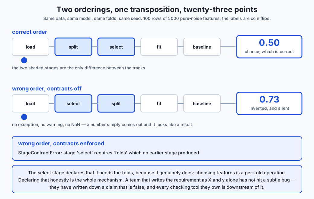
Here are two runs of the same pipeline, on the same data, with the same model, the same folds and the same seed.
split then select (correct)            : 0.5000
select then split (wrong, unchecked)   : 0.7300
accuracy invented by the reordering    : 0.2300
The dataset is one hundred rows and five thousand columns of numbers drawn from a normal distribution, and the labels are coin flips. There is nothing to learn. Not a weak signal, not a subtle one — nothing, by construction, because the labels were never produced by looking at the features.
The correct pipeline reports 0.50. That is chance, and chance is the only honest answer available.
The other pipeline reports 0.73, and the difference between them is that two stages changed places:
correct order : load -> split -> select -> fit_and_score -> baseline
wrong order   : load -> select -> split -> fit_and_score -> baseline
That is the whole diff. select moved in front of split. No exception
was raised. No warning was printed. No value came back as NaN. A number
simply came out, and it looks exactly like a result — better than chance,
plausible for a hard problem, the sort of figure that goes on a slide.
You have met leakage before, on Day 137, as a concept: information about the answer reaching the model. Today it arrives as something more uncomfortable, which is that leakage is usually not a mistake in reasoning. It is a mistake in ordering — and ordering is precisely the thing that a notebook, a pile of scripts, or a diagram of boxes with arrows does not enforce.
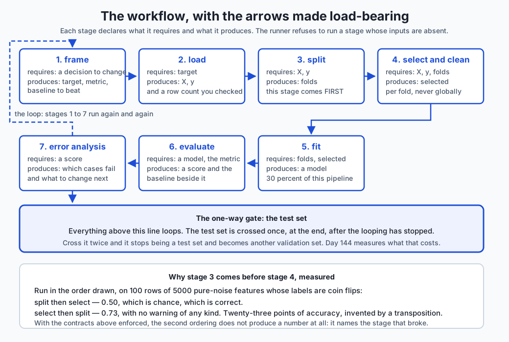
Today’s lab makes the ordering enforceable. Every stage declares what it requires and what it produces; the runner refuses to run a stage whose inputs are absent. Run the same wrong pipeline with those contracts switched on and you do not get 0.73:
StageContractError: stage 'select' requires ['folds'] which no earlier
stage produced
That is the subject of the day. Not the list of stages — you could recite those already — but what has to be true of the connections between them for the number at the end to mean anything.
The idea in plain language
Think about a recipe with a step that says “fold in the egg whites”.
That step depends on an earlier one, “beat the egg whites to soft peaks”, and the dependency is not a matter of taste. Perform them in the other order and you do not get a slightly worse cake. You get something that is not a cake, and — this is the part that matters — you find out much later, from the oven, in a form that does not tell you which step was wrong.
A recipe handles this by being a numbered list that a human reads in order. That works because the steps are short, the cook is present, and the failure is spectacular.
A machine learning pipeline has none of those advantages. The steps are long. Nobody is watching most of the time. And the failure is not spectacular at all: it is a number that is slightly too good, which is the one kind of bad news that nobody investigates.
So the workflow needs something the recipe does not: each step has to declare its own dependencies, so that running them out of order is detected by the machinery rather than noticed by a person.
That is the difference between a workflow you have drawn and a workflow you have wired up. Drawn workflows are documentation, and documentation does not run. A wired-up workflow is code that fails when the ordering is wrong.
Historical background
The workflow was written down as a process long before machine learning had a workflow worth writing down, and the reason is that it was not invented for machine learning.
CRISP-DM — the Cross-Industry Standard Process for Data Mining — was published in 1999 by a consortium including Daimler-Chrysler, SPSS and NCR. Its six phases are business understanding, data understanding, data preparation, modelling, evaluation and deployment, drawn as a circle because the process was understood from the start as a loop rather than a line. It remains, more than twenty-five years later, the most widely recognised description of the thing, and its longest-lasting contribution is the ordering of the first two phases: understand the business problem before the data, and the data before the model.
SEMMA, from the SAS Institute in the same era, took a narrower view — sample, explore, modify, model, assess — and is more tightly bound to tooling. The two are usually presented as rivals; the difference that matters is that CRISP-DM begins outside the data and SEMMA begins inside it, which is a disagreement about whether framing is part of the job.
What neither had was a way to enforce anything, because they were
methodologies rather than software. That gap took much longer to close.
scikit-learn’s Pipeline object, which makes the correct ordering of
preprocessing and model fitting structural rather than advisory, arrived
in the library’s early years and is the single most important practical
contribution to this problem. It exists precisely because the wrong
ordering was so common and so silent.
The measurement in this lesson also has a literature. Ambroise and McLachlan published a paper in 2002 on selection bias in gene-expression classification, showing that choosing features on the full dataset before cross-validating produced dramatically optimistic error rates — on microarray data where the number of features vastly exceeds the number of samples, which is exactly the shape of today’s noise dataset. The Elements of Statistical Learning devotes a section to it under the heading of the wrong and right ways to do cross-validation, and it is still being rediscovered in published work every year.
The last decade added the operational half. The phrase “technical debt in machine learning systems” comes from a 2015 paper by a team at Google arguing that the model code is a small box in the middle of a much larger system, and the MLOps tooling that followed — pipeline orchestrators, feature stores, model registries — is mostly an attempt to make the non-modelling parts of this workflow reproducible.
What it is — and what it is not
The workflow is a loop around a one-way gate.
The loop is stages one through seven: frame the problem, get the data, split it, prepare features, fit, evaluate, analyse the errors, and go round again with what you learned. You will traverse that loop many times. It is supposed to be traversed many times.
The gate is the test set. It is crossed once, at the end, after the looping has stopped. Everything inside the loop is fair game to iterate on; the moment the test set enters the loop it stops being a test set and becomes another validation set, and you no longer have an unbiased estimate of anything. Day 144 measures what that costs.
Now the things it is not.
It is not a linear sequence. Every honest account of the process describes going backwards. Error analysis sends you back to feature preparation. Feature work reveals that the data you loaded does not support the target you framed. Evaluation reveals that the metric you chose is not the one anyone cares about. The arrows in the diagram point both ways, and a workflow drawn as a straight line is a workflow that has not been run.
It is not mostly modelling. This claim usually arrives as folklore with a percentage attached, and the percentages disagree with each other, so today’s lab measures its own pipeline instead:
    load             5 lines
    split            2 lines
    select          10 lines
    fit_and_score    9 lines
    baseline         4 lines
    total           30 lines
  the fitting stage is 30.00% of this pipeline
Thirty percent — and that is an upper bound, not an estimate, because this pipeline is deliberately minimal. It has no data cleaning stage. It has no monitoring, no deployment, no schema validation, no drift detection, and no code at all for the part where somebody decides what the target should be. Every one of those additions makes the modelling fraction smaller. What the measurement establishes is a direction, and the direction is enough.
It is not a set of stages that can be run in any order that produces output. This is the failure the whole day is built around, and it is worth being precise about why it is so easy to commit. The wrong ordering does not produce an error, does not produce a warning, and does not produce an implausible number. It produces a better number, which means the ordinary feedback loop of software development — try it, see if it looks right — is actively pointing the wrong way.
And it is not finished when the model is good. A model that is never deployed has produced nothing. A model that is deployed and never monitored will decay, because the world moves and the training distribution does not.
Why it was created and what problems it solves
Each stage exists because a specific, expensive failure happens when it is missing. That is the useful way to hold the list in your head: not as seven things to do, but as seven failures somebody already paid for.
Framing exists because projects solve the wrong problem. The stage produces three things — the target, the metric, and the baseline to beat — and all three have to be settled before any model exists, because all three determine which model you would ship.
The metric especially. Here are five candidates on an imbalanced problem where eight percent of rows are positive:
| Model | accuracy | precision | recall | F1 |
|---|---|---|---|---|
| majority baseline | 0.9200 | 0.0000 | 0.0000 | 0.0000 |
| logistic (default threshold) | 0.9435 | 0.7196 | 0.4813 | 0.5768 |
| logistic (balanced) | 0.8685 | 0.3619 | 0.8438 | 0.5066 |
| 5-NN | 0.9360 | 0.6739 | 0.3875 | 0.4921 |
| depth-3 tree | 0.9275 | 0.6027 | 0.2750 | 0.3777 |
Read that table twice, once down the accuracy column and once down the recall column, and you have selected two different models. Accuracy ships the default-threshold logistic regression. Recall ships the balanced one — which is, on accuracy, the worst model in the table and the only one that loses to a constant.
The metric was not a reporting decision. It was the decision.
Baselines exist because scores have no absolute meaning. The first row of that table is a model that always predicts the majority class. It has learned nothing, cannot possibly be useful, and scores 0.92. The three real models that beat it do so by at most 2.35 points. Without that row, 0.9435 reads as an excellent result; with it, it reads as two and a bit points of value that you now have to justify against the cost of maintaining a model.
Splitting exists because a model can memorise, which Day 141 measured, and Day 144 covers properly.
Careful stage ordering exists because of the 0.73. That is this lesson’s contribution and the rest of it is spent there.
Error analysis exists because an aggregate hides everything. The 0.9435 model, broken down:
  rows = true class, columns = predicted class
    true 0: [1810, 30]
    true 1: [83, 77]
Ninety-four percent accurate, and it misses eighty-three positives while catching seventy-seven. It finds fewer than half of the thing it exists to find. One number told you it was good. Four numbers told you what it does.
Reproducibility exists because you will need to know whether something changed. A pipeline that cannot prove it produced the same output twice cannot be debugged, because you can never distinguish a fix from a coincidence.
How it works
A stage is a contract, not a cell in a notebook
Here is the whole idea in one dataclass:
@dataclass
class Stage:
    name: str
    run: Callable[[Artifact], dict]
    requires: tuple = ()
    produces: tuple = ()
And the runner:
for stage in stages:
    if enforce_contracts:
        missing = [k for k in stage.requires if k not in artifact.data]
        if missing:
            raise StageContractError(
                f"stage {stage.name!r} requires {missing} which no earlier stage produced"
            )
    produced = stage.run(artifact)
    artifact = artifact.with_(**produced)
    artifact.log.append((stage.name, tuple(sorted(produced))))
Four things in that loop are doing real work, and each is a decision worth defending.
The check runs before the stage, not after. A stage that has already half-run and then fails leaves you reasoning about a partially-mutated state. Checking first means a stage either runs completely or does not start.
with_ returns a new artifact rather than mutating in place. This is
not functional-programming decoration. A stage that mutates its input
makes the step log a work of fiction, because the log then describes
states that no longer exist. An audit trail that can be rewritten by the
thing it audits is not an audit trail.
The log records what each stage produced, not what it was asked to do. Intent is cheap. The step log for the honest pipeline:
    load           -> X, y
    split          -> folds
    select         -> selected
    fit_and_score  -> fold_scores, score
    baseline       -> baseline
And the contract is checked in both directions. A stage that fails to produce what it declared raises; so does one that produces something extra. The second is easy to dismiss and worth keeping, because undeclared outputs are how a pipeline accumulates hidden coupling that nobody can see in the code.
The measurement: two stages, transposed
Now the central experiment. The dataset is deliberately hostile in a specific way: one hundred rows, five thousand features, labels from a coin flip. Five thousand columns of noise and one hundred rows means that by pure chance, some columns will correlate with the labels quite well. Not because they mean anything — because with five thousand attempts at a coin flip, some sequences match.
The wrong pipeline:
chosen = top_k_features(X, y, k)          # uses every row, including test rows
for train, test in folds(X, y):
    model = KNeighborsClassifier(1).fit(X[train][:, chosen], y[train])
The right one:
for train, test in folds(X, y):
    chosen = top_k_features(X[train], y[train], k)   # training rows only
    model = KNeighborsClassifier(1).fit(X[train][:, chosen], y[train])
In the first, every fold’s test rows helped choose the features. The features were fitted to the answers before the answers were hidden. The model then legitimately does well on those test rows, because they were consulted when deciding what to look at.
Note what is not wrong with the first version. The model never sees a test label during fitting. The folds are correct and disjoint. The cross-validation loop is textbook. Every individual piece is right, and the composition is wrong — which is why reviewing the model code line by line will never find it.
How big the lie gets
The twenty-three points are not a fixed penalty. They depend on how many features you select, and the relationship is worth seeing:
| features chosen | wrong order | right order | invented |
|---|---|---|---|
| 5 | 0.6500 | 0.3900 | +0.2600 |
| 10 | 0.7200 | 0.5000 | +0.2200 |
| 20 | 0.7300 | 0.5000 | +0.2300 |
| 50 | 0.8500 | 0.3800 | +0.4700 |
At fifty features the wrong ordering reports eighty-five percent accuracy on data that contains nothing. There is no shape of that curve that makes the wrong order safe.
One honest note about that table, because it would be easy to skate past: two of the right-order scores are below chance, at 0.39 and 0.38. That is not anti-learning and it is not a bug. With one hundred rows split five ways, each fold’s score is measured on twenty rows, giving a standard error near 0.11 around a true value of 0.5. An estimate that wanders will wander below as readily as above — Day 117’s arithmetic, arriving where it matters. The lab therefore asserts that the honest score is at or below chance rather than exactly 0.5, because that is the claim the evidence actually supports.
The contract is a declaration, and declarations can be false
This is the part of the day most likely to be misread, so it is worth being blunt about it.
The select stage in the leaky pipeline still declares folds among its
requirements:
Stage(
    "select",
    _stage_leaky_select,
    requires=("X", "y", "folds", "k"),
    produces=("selected",),
)
That requirement is true. Choosing features is a per-fold operation. Declaring it honestly is the entire mechanism by which the runner can notice that the stage has been placed too early.
Which means the contract does not protect you from a team that writes
requires=("X", "y") on that stage. Nothing does. But that team has not
been caught out by a subtle bug — they have written down a claim that is
false, in a file, where somebody can read it and disagree. That is a
categorically better position than a notebook where the dependency was
never stated at all and exists only in the order the cells were run.
The value of a contract is that it turns an implicit ordering into a reviewable claim. It does not make wrong claims impossible. It makes them visible.
Reproducibility: proving the pipeline did the same thing twice
The last piece of machinery is a manifest of content hashes:
def fingerprint(value) -> str:
    if isinstance(value, np.ndarray):
        payload = np.ascontiguousarray(value).tobytes() + str(value.dtype).encode()
    else:
        payload = repr(value).encode()
    return hashlib.sha256(payload).hexdigest()[:16]
Run the honest pipeline twice at seed 143 and once at seed 144:
    X            51b0a421bd652dd2
    fold_scores  8f0ac332958b9bc4
    score        d2cbad71ff333de6
    y            9984503b5352c5a1
  two runs at seed 143 agree             : True
  a run at seed 144 differs              : True
The second line is the claim. The third line is what makes the second line mean anything, and it is the check people leave out. A manifest that always matches might be proving determinism, or it might be proving that you are hashing a constant, and only a deliberate change can tell you which.
One detail in fingerprint is deliberate and worth copying: the dtype is
part of the hash. The same numbers stored as int64 and as float64 hash
differently, on purpose, because treating them as the same artifact would
hide a real class of bug. Silently-equal hashes are worse than no hashes.
Failing well
The last thing the contracts buy is the quality of the failure. Run the honest pipeline against an empty artifact, with contracts on and off:
with contracts on : StageContractError: stage 'load' requires
                    ['n_samples', 'n_features', 'seed'] ...
with contracts off: KeyError: 'n_samples'
Both fail. Only one tells you which stage broke and what it wanted. The
KeyError names a dictionary key from somewhere inside a function you now
have to go and find, and in a pipeline of thirty stages that difference is
most of your afternoon.
An everyday analogy
Consider a hospital laboratory processing a blood sample.
The sample arrives, is labelled, is split into aliquots, and each aliquot goes to a different test. Results come back, get read against reference ranges, and a report goes to a clinician. That is a workflow, and it looks very like the one in this lesson.
Now consider what a laboratory does that a notebook does not.
Every step has a chain of custody. Not because anyone distrusts the technicians, but because when a result is surprising, the first question is what happened to the sample — and “I think I did them in the usual order” is not an answer. That is the step log.
Steps that must precede other steps are physically enforced wherever possible. The aliquots are split before any reagent is added, and they are split by a machine whose sequence you cannot reorder by accident. That is the stage contract.
Controls are run alongside the sample. A known-negative and a known-positive go through the same process, every batch. If the known-negative comes back positive, the batch is void — regardless of how plausible the patient results look. That is the baseline, and it is also the noise dataset in today’s lab: a known-negative put through the pipeline, so that a pipeline reporting 0.73 on it is known to be broken without needing to argue about the real data.
The analogy earns its keep at that last point. Everybody accepts that a laboratory runs controls. Almost nobody runs a control through their machine learning pipeline — feeds it data with a known answer of “there is nothing here” and checks that it says so. It costs about four lines. It would have caught the 0.73.
Examples in practice
The framing stage, done properly
A team is asked to “reduce customer churn with machine learning”. The framing stage turns that into three artifacts before anybody writes code:
- The target. Churn defined how? Cancelled within thirty days of renewal? Ninety? Stopped using the product but still paying? Each is a different column and a different project.
- The metric. If the intervention is a discount email costing very little, recall matters and precision barely does. If it is a phone call from a named account manager, precision is the constraint. The table earlier in this lesson is what that choice looks like in numbers.
- The baseline. What does the current process achieve? If the sales team already calls everyone whose usage dropped, that is the baseline, and it may be hard to beat.
Skipping this stage does not feel like skipping anything, which is exactly why it gets skipped. There is no error message for “you built a model for the wrong target”.
Stage ordering, in the tools that get it right
scikit-learn’s Pipeline exists to make today’s failure structurally
impossible:
from sklearn.pipeline import Pipeline
from sklearn.feature_selection import SelectKBest, f_classif

pipe = Pipeline([
    ("select", SelectKBest(f_classif, k=20)),
    ("model", KNeighborsClassifier(1)),
])
cross_val_score(pipe, X, y, cv=5)
The mechanism is worth understanding rather than memorising. Pipeline
delays every fit until it is inside the cross-validation fold. The
selection step is fitted on the training rows of each fold and only
transform-ed on the test rows, so there is no arrangement of this code
in which the test rows influence the selection.
This is the same idea as today’s stage contract, implemented once, in a library, by people who had seen the failure enough times to build against it.
Error analysis, and what it changes
Return to the confusion matrix. Eighty-three false negatives against seventy-seven true positives. What does an analyst do next?
Not “try a better model”. They ask which eighty-three. Are they the borderline cases near the decision boundary, in which case moving the threshold is the whole fix and no new model is needed? Are they a recognisable subgroup, in which case there is a missing feature? Are they mislabelled, in which case the ceiling is lower than anyone thinks?
Three different answers, three different next stages, and the aggregate score distinguishes none of them. Error analysis is the stage that decides what the next loop is for.
What the eight measurements say together
The lab’s numbers make one argument. A workflow is not the list of its stages, because the same stages in a different order gave 0.50 and 0.73. It is not the modelling either, which was thirty percent of a pipeline with no cleaning or deployment in it. It is the connections: what each stage may assume, what it must produce, what crosses the gate and when. Get those right and the number at the end means something. Get them wrong and it means nothing, quietly.
Implications: security, privacy, performance, scalability, and cost
The most expensive property of the ordering bug is when you find out. A model that reports 0.73 in development, ships, and delivers 0.50 in production has cost the build, the review, the deployment, the incident, and the credibility of the next project. The contract check costs microseconds and runs on every execution.
Reproducibility is a security control, not only a scientific one. The manifest in today’s lab is the same primitive as a package lock file, a container digest, or a signed release artifact, and it answers the same question: is what I have now the thing I checked before? A pipeline that cannot answer that cannot be audited, and “the notebook I ran in March” is not an answer to a regulator, a reviewer, or a colleague in two years.
Privacy attaches to the split, and it is the stage where it is easiest to get wrong. If your rows are people and the same person appears in both halves, your test set is not held out and your model may be memorising individuals — which is both an evaluation failure and a disclosure risk. Day 144 measures the evaluation half.
The step log is an access-control surface. It records what data entered which stage. That is exactly what a data protection review needs and exactly what a notebook cannot provide.
Performance and scalability favour the contract-checked design, which is not obvious and is worth stating. The check is a set difference over a handful of strings, and it runs once per stage rather than once per row. Against that, it makes stages independently cacheable — a stage whose declared inputs have not changed does not need to run again, which is exactly how a pipeline orchestrator avoids recomputing the expensive parts. The contract that catches the bug is also the thing that makes the caching sound.
And the cost that is hardest to see is the cost of the loop. Every traversal is a chance to learn something and also a chance to overfit your own judgement to the validation set — Day 136’s forking paths. The gate exists to bound that, and the discipline it demands is the unglamorous one: decide what you are going to try before you try it, and count how many times you have gone round.
Alternatives: free, open source, and commercial
A hand-written stage runner — used here
When to choose it: when you want the contract to be visible and auditable, when your stages are heterogeneous enough that a library’s abstractions do not fit, or — as here — when the point is to understand what the abstraction is doing for you.
How to use it: the entire runner is about forty lines and appears in this lesson. It is genuinely enough for a small project.
Watch for: it enforces only what you declare. That is the honest limitation and it is discussed above at length.
scikit-learn’s Pipeline — used here
When to choose it: for any preprocessing that must be fitted, which is almost all of it — scaling, imputation, encoding, feature selection, dimensionality reduction. It is free, BSD-3-Clause licensed, no paid tier.
How to use it: compose the steps and hand the whole thing to
cross_val_score, GridSearchCV or fit, as shown earlier. Use
ColumnTransformer when different columns need different treatment.
Watch for: Pipeline protects the steps inside it. Anything you did
to the data before constructing it — dropping rows, imputing a column,
selecting features by eye in a notebook cell — is outside the protection
and is exactly where the leak comes back.
Kedro, Metaflow and Prefect — not installed here, described from documentation
These are free, open-source project-scale pipeline frameworks, and they solve the same problem this lesson solves with forty lines, at the scale where forty lines stops being enough.
When to choose one: when stages must run on different machines, when you need caching of expensive stages across runs, when a schedule and a retry policy are involved, or when more than one person is editing the pipeline. Kedro is the most opinionated about project structure; Metaflow came out of a data-science-workflow context and emphasises versioning of runs; Prefect is a general orchestrator with strong scheduling and failure handling.
Honest note: none of these is installed on the authoring machine and no output from any of them is reproduced anywhere in this lesson. Everything stated about them comes from their published documentation.
Managed MLOps platforms — not used here, described from documentation
The major cloud providers all sell platforms combining pipeline orchestration, experiment tracking, a model registry and monitoring.
When to choose one: when the operational half of the workflow — deployment, monitoring, rollback, audit — is the hard part, and when you would otherwise be building it yourself.
When not to: at the stage where you are still finding out whether the problem is tractable. The workflow in this lesson runs on a laptop, and it is the same workflow.
Free versus paid: all are paid, generally metered on compute plus storage plus per-endpoint charges. No price is quoted here, because cloud pricing changes by region and by month and an unchecked figure is worse than none.
Comparison with related concepts
| Concept | What it governs | How it relates to this workflow |
|---|---|---|
| CRISP-DM | the phases of a data-mining project | The ancestor of this diagram; a methodology, with no way to enforce anything |
| ETL / ELT pipelines | moving and reshaping data | The same ordering discipline, one stage earlier; Day 126 built one |
| CI/CD | building and shipping software | Where the “prove it runs the same way twice” habit comes from; the manifest is a lock file |
sklearn.pipeline.Pipeline | preprocessing plus a model, as one object | The stage contract, implemented in a library and made structural |
| MLOps | the operational half — deploy, monitor, retrain | The stages this lesson names but does not build, which is why its 30 percent is an upper bound |
| Experiment tracking | recording what you tried and what happened | The step log and manifest, scaled up and made searchable |
| Feature stores | computing features once, consistently | An answer to a specific ordering bug: features computed differently at training and serving time |
The last row deserves a note, because it is the same bug as today’s in a
different costume. Training-serving skew happens when the feature
computed during training and the feature computed at prediction time are
not the same function — a rolling average over a window that includes the
present in training and excludes it in production, say. It is silent, it
inflates the offline number, and it is found only when live performance
disappoints. A feature store exists so that one definition serves both,
which is the structural fix, exactly as Pipeline is the structural fix
for the leak measured today.
When to use it — and when not to
Use the full workflow, with contracts, when the result will be acted on. If a number you produce will change a decision, somebody is entitled to ask how it was produced, and you should be able to answer with a step log rather than a memory.
Use it especially when the data is wide. Today’s dataset — one hundred rows, five thousand features — is the shape where selection bias is enormous, and it is a real shape: genomics, sensor arrays, text with n-gram features, anything with more columns than rows. The inflation reached forty-seven points.
You do not need the full apparatus for exploration. A notebook where you look at distributions and form hypotheses is a legitimate and valuable thing, and wrapping it in stage contracts would slow it down for no benefit. The rule is about the boundary: the moment a number leaves the notebook and enters a conversation, it needs to have come through the wired-up pipeline. A finding is not a result.
Do not use a heavyweight orchestrator too early. The workflow in today’s lab runs on a laptop in a few seconds, and it is the same workflow a platform would run. Adopting a framework before you know your stages means designing your project around somebody else’s abstraction of a problem you have not met yet.
And do not skip the framing stage because it produces no code. It is the only stage whose omission has no error message. Every other failure in this lesson eventually announces itself; a model built for the wrong target can go to production and work perfectly.
The AI thread
The workflow does not disappear when the model is a large language model. It changes shape in one specific way, and understanding which way is most of what distinguishes competent LLM engineering from prompt-tinkering.
The framing stage is unchanged and becomes more important, because the model will produce fluent output for a badly-framed task and the output’s fluency conceals the framing error.
The splitting stage becomes harder in a way that is worth naming plainly. Your evaluation set must be data the model has not seen — and the model was trained on a large fraction of the public internet. A benchmark published before the model’s cutoff may well be in its training data, and a score on it is then measuring memorisation. This is Day 141’s leakage and today’s ordering problem combined, at a scale where you cannot inspect the training set to check.
The metric stage is where most of the difficulty moves. There is no
accuracy_score for “was this summary good”. So the metric becomes a
rubric applied by human raters, or by another model acting as judge — and
that judge is itself a model with its own biases, which need their own
evaluation. The table in this lesson, where the metric decided which model
shipped, applies with more force when the metric is itself a learned
thing.
Error analysis becomes the highest-leverage stage of the lot. Reading a hundred actual failures of an LLM system tells you more than any aggregate score, because the failure modes are categorical — refuses when it should answer, hallucinates a citation, ignores half the instruction — and each one has a different fix.
And the contract idea transfers directly. A retrieval-augmented system is a pipeline: retrieve, rank, assemble a context, generate, post-process. Every one of those stages has inputs it requires and outputs it promises, and every one of them can be silently mis-ordered. The 0.73 has an exact analogue: an evaluation where the retrieval step was tuned using the same questions the system was later scored on. Same bug, same silence, same fix.
Knowledge check
- Two pipelines share their data, model, folds and seed, and differ only
in that one runs
selectbeforesplit. One reports 0.50 and the other 0.73 on data whose labels are coin flips. Explain the mechanism in one sentence, and say why reviewing the model code would not find it. - The
selectstage in the leaky pipeline declares that it requiresfolds. Why is that declaration the thing that makes the mis-ordering detectable, and what does it fail to protect against? - A model scores 0.9435 accuracy. The majority-class baseline scores 0.9200. What have you learned, and what would you need to know next?
- Give a case where a model with lower accuracy than a constant is the right one to ship, using the table in this lesson.
- A pipeline’s manifest is identical on every run. Name the two different situations that could produce that, and the one check that distinguishes them.
- Why does the runner check a stage’s requirements before running it rather than catching the resulting exception?
- This lesson measured the fitting stage at 30% of its pipeline and called that an upper bound rather than an estimate. Justify the word “upper”.
- Two of the honest cross-validation scores in the inflation table are below 0.5. Explain why that is expected, and why the lab asserts an inequality rather than a value.
Hands-on exercise
Today’s lab, The Workflow, Wired Up, builds the workflow as stages with
declared contracts, then measures what the ordering is worth.
Thirteen exercises. The first half establishes the machinery — the step log, the immutable artifact, the contract in both directions — and then transposes two stages and measures the twenty-three points. The second half is the decisions the machinery exists to support: the metric, the baseline, the confusion matrix, and a manifest that proves determinism.
Build the environment, then work through
starter/test_workflow_claims.py, replacing one pytest.skip at a time.
Each skip names the exact helper and the exact value to assert.
Expected output
The harness ends with:
---------------------------------------------------------------
14 checks, 0 failure(s)
and exits 0. pytest examples -q reports 17 passed, and
pytest starter -q reports 4 passed, 13 skipped until you begin.
The measured table, printed by examples/report_measurements.py,
includes:
  split then select (correct)            : 0.5000
  select then split (wrong, unchecked)   : 0.7300
  accuracy invented by the reordering    : 0.2300
  with contracts enforced                : StageContractError
    stage 'select' requires ['folds'] which no earlier stage produced
  two runs at seed 143 agree             : True
  a run at seed 144 differs              : True
Validate your work
bash tests/run_tests.sh; echo "exit=$?"reports14 checks, 0 failure(s)andexit=0. Capture the harness’s own exit status, never a pipeline’s..venv/bin/pytest examples -qreports17 passed..venv/bin/python3 examples/report_measurements.py | diff - expected-output/measured-values.txtproduces no output.- When you have finished every exercise,
pytest starter -qalso reports17 passed. - Break one assertion on purpose, confirm the harness reports the failure and exits non-zero, and restore it.
Troubleshooting
StageContractError when you did not expect one. Read the message: it
names the stage and the missing key. If you are running leaky_stages()
with contracts on, that error is the expected result.
A bare KeyError from inside a stage. You ran with
enforce_contracts=False. Both paths fail; only one tells you which stage
broke. Exercise 8 asserts both, side by side.
import file mismatch. You ran pytest examples starter in one
invocation. Run them separately — check 5 asserts that the combined form
fails.
An honest score below 0.5. Expected. Twenty test rows per fold gives a
standard error near 0.11. The lab asserts right <= 0.5 for that reason.
Manifest hashes that do not match. Read expected-output/FIELDS.md.
The hashes are over exact float bytes and move with the NumPy pin; the
property that must hold anywhere is that two runs agree and two seeds do
not.
Common mistakes
Reading the 0.73 as a modelling problem. It is not. The model, the folds and the data are identical in both runs. Only the order changed.
Declaring a stage’s requirements as whatever makes the pipeline run. That inverts the whole point. The requirement is a claim about what the stage genuinely depends on, and getting it right is the work.
Asserting the manifest matches without asserting a different seed differs. The second check is what makes the first mean anything.
Skipping exercise 4 because the numbers look boring. That table is the day’s most consequential result: two metrics, five models, two different answers about what to ship.
Practice assignment
Take a pipeline you already have — a notebook, a script, or a chain of scripts — and convert its first five stages into declared contracts.
- Write down each stage’s
requiresandproducesbefore looking at the code. Then check the code against them. Note every place they disagree; each disagreement is either a wrong declaration or a hidden dependency, and both are findings. - Find the stage that is fitted. Anything that learns from data — a scaler, an imputer, an encoder, a feature selector, a threshold — and confirm it is fitted on training rows only. If you cannot tell from the code, that is your answer.
- Run a control. Replace your labels with a random permutation, run the whole pipeline, and record the score. Anything meaningfully above your baseline is a bug report. This is four lines and it is the single highest-value thing in this assignment.
- Add a manifest. Hash your inputs and your final score. Run twice, confirm they match. Then change the seed and confirm they do not.
- Write down your metric and your baseline, in that order, before looking at any model score. If you cannot state why that metric and not another, the framing stage is not finished.
The deliverable is the contract table, the control result, and the manifest — not a better model.
Extension challenge
Pick one and measure it. Report what you observed rather than what you expected.
- Make the leak pass its contracts, dishonestly. Change
selectto declarerequires=("X", "y", "k")and watch the whole pipeline run green at 0.73. Then write two sentences on what that tells you about where the real control lives. - Replace the runner with
sklearn.pipeline.Pipeline. Wrap selection and model together, pass it tocross_val_score, and confirm the honest number. Explain which property ofPipelinemakes the leak impossible rather than merely unlikely. - Sweep the threshold. Instead of comparing default against balanced
class weights, sweep the decision threshold with
predict_probafrom 0.05 to 0.95 and report the threshold maximising F1. Compare it to both models in the lesson’s table. - Break determinism on purpose. Remove
random_statefrom theStratifiedKFold, confirm the manifest stops matching, and then say what you would have concluded had you found that in a real project with no manifest to tell you. - Find the worst k. Sweep the number of selected features from 5 to 100 and find where the invented accuracy is largest. Explain the shape of the curve in terms of how many chances the selector gets.
- Add the missing stages. Add a cleaning stage and a monitoring stage
with honest contracts, re-measure
stage_source_lines, and report how far the modelling fraction falls below 30 percent.
Quiz
Q1. Two pipelines share their data, their model, their folds and their seed. One runs `select` before `split` and reports 0.73; the other runs `split` before `select` and reports 0.50. The labels are coin flips. What produced the 0.23?
- The leaky pipeline reuses one global feature selection across folds, so the folds are no longer independent of each other
- Every fold's test rows helped choose the features, so the features were fitted to the answers before the answers were hidden
- The 1-NN model memorises its training rows, and the wrong ordering gives it more of them
- Five-fold cross-validation is biased on small samples, and the leaky pipeline happens to expose that bias
Show answer
Answer: B. Every fold's test rows helped choose the features, so the features were fitted to the answers before the answers were hidden
With 5000 noise columns and 100 rows, some columns will correlate with the labels by pure chance. Choosing the top twenty using every row means the test rows of every fold voted on which columns to look at, so the model does legitimately well on them. Note what is NOT wrong: the model never sees a test label during fitting, the folds are disjoint and correct, and the cross-validation loop is textbook. Every individual piece is right and the composition is wrong, which is exactly why reviewing the model code line by line never finds it.
Q2. In the leaky pipeline, the `select` stage still declares `folds` among its requirements. Why does that matter?
- It does not really matter; the runner could infer the dependency from which keys the stage function reads
- It documents the stage for future readers, which is good practice but not load-bearing
- It is what lets the runner notice the stage was placed too early -- the declaration is true, and checking a true declaration against the keys present is the whole mechanism
- It makes the stage fail faster, which reduces wasted compute on large datasets
Show answer
Answer: C. It is what lets the runner notice the stage was placed too early -- the declaration is true, and checking a true declaration against the keys present is the whole mechanism
Choosing features genuinely is a per-fold operation, so `folds` genuinely is a requirement. Stating it honestly is what turns an implicit ordering into a checkable claim. Inferring dependencies from what the function reads is not equivalent -- the leaky stage reads only X and y, so inference would conclude, correctly and uselessly, that it can run first. And note the limitation this implies: a team that writes `requires=("X", "y")` defeats the check entirely. The contract does not make wrong claims impossible; it makes them visible.
Q3. A model scores 0.9435 accuracy on a problem where 8 percent of rows are positive. The majority-class baseline scores 0.9200. What have you learned?
- That the model is 94 percent accurate, which is a strong result on an imbalanced problem
- That the model has learned nothing, since 0.9435 is close to the base rate
- That the model is well calibrated, since its accuracy tracks the class distribution
- That the model adds 2.35 points over a constant -- and nothing yet about whether those points are the ones anybody wanted
Show answer
Answer: D. That the model adds 2.35 points over a constant -- and nothing yet about whether those points are the ones anybody wanted
The baseline turns an impressive-looking 0.9435 into a modest 2.35-point improvement that now has to justify the cost of building and maintaining a model. But the gap is only half the story: this same model catches 77 of 160 positives and misses 83. Concluding it has learned nothing is too strong -- 0.7196 precision is real -- and calibration is a different property entirely, about predicted probabilities rather than accuracy. The honest summary is "2.35 points, on a metric that may be the wrong one".
Q4. When would you ship a model with lower accuracy than a majority-class baseline?
- When recall is what the decision needs -- the balanced logistic model scores 0.8685 accuracy against the constant's 0.9200, and catches 84 percent of positives against the constant's zero
- Never; accuracy below a constant means the model is worse than doing nothing
- When the training accuracy is higher, indicating the model has capacity the test set cannot show
- When the dataset is imbalanced, because accuracy is undefined on imbalanced data
Show answer
Answer: A. When recall is what the decision needs -- the balanced logistic model scores 0.8685 accuracy against the constant's 0.9200, and catches 84 percent of positives against the constant's zero
The constant scores 0.92 by never predicting a positive, so it catches none of the thing the system exists to catch. If the intervention is cheap -- an email, a flag for review -- 0.8438 recall at 0.3619 precision is straightforwardly more valuable than 0.92 accuracy at zero recall. Accuracy is perfectly well defined on imbalanced data; it is just answering a question nobody asked. And training accuracy is never the argument, which Day 141 measured at length.
Q5. Your pipeline's manifest of content hashes is identical on every run. What does that establish?
- That the pipeline is deterministic, which is the property you wanted
- Either that the pipeline is deterministic, or that you are hashing something that never varies -- and only changing an input can tell you which
- That the pipeline is correct, since a correct pipeline produces stable output
- That the random seed is being applied, since an unseeded pipeline would produce different hashes
Show answer
Answer: B. Either that the pipeline is deterministic, or that you are hashing something that never varies -- and only changing an input can tell you which
This is the control that gets left out. A manifest that always matches might be proving determinism or might be proving that the thing you hashed is a constant -- a typo in the key name, a stage that silently returns the same empty array, a hash taken before the varying step. The lab therefore asserts both directions: two runs at seed 143 agree AND a run at seed 144 differs. Determinism says nothing about correctness; a reliably wrong pipeline is reliably wrong.
Q6. Why does the stage runner check a stage's declared requirements *before* running it, rather than letting the stage fail and catching the exception?
- Because exceptions are slow in Python, and the check runs on every stage of every execution
- Because catching exceptions would swallow genuine errors from inside the stage as well
- A stage that half-runs and then fails leaves a partially-mutated state to reason about; checking first means a stage either runs completely or never starts
- Because the exception type varies by stage, so there is nothing reliable to catch
Show answer
Answer: C. A stage that half-runs and then fails leaves a partially-mutated state to reason about; checking first means a stage either runs completely or never starts
The atomicity is the point. It also produces a categorically better error: `StageContractError: stage 'load' requires ['n_samples', ...]` names the stage and what it wanted, while the uncaught version gives you `KeyError: 'n_samples'` from somewhere inside a function you now have to find. In a thirty-stage pipeline that difference is most of an afternoon. Exception cost is irrelevant at this scale, and conflating genuine stage errors with contract violations is a real concern but a consequence of the design rather than its motivation.
Q7. This lesson measured its fitting stage at 30 percent of the pipeline and called that an upper bound rather than an estimate. Why "upper"?
- Because line counts overstate the size of the fitting stage, which is denser than the others
- Because a larger dataset would need more loading code, lowering the fraction
- Because 30 percent is above the commonly quoted figure, so the true value must be lower
- Because this pipeline has no cleaning, monitoring, deployment, schema-validation or drift-detection stage, and every one of those would be added to the denominator
Show answer
Answer: D. Because this pipeline has no cleaning, monitoring, deployment, schema-validation or drift-detection stage, and every one of those would be added to the denominator
The measurement is of a deliberately minimal pipeline, so every stage a real project would add makes the modelling fraction smaller and none makes it larger. That is what licenses the word "upper". The lesson measures its own pipeline rather than quoting the familiar percentage precisely because the familiar percentages disagree with each other and none could be verified here -- a direction that is defensible beats a number that is not.
Q8. Two of the honest cross-validation scores in the lab's inflation table are below 0.5, at 0.39 and 0.38. What is the right response?
- None -- with 20 test rows per fold the standard error is near 0.11, so an estimate of a 0.5 quantity wanders below as readily as above
- Investigate: scoring below chance means the model has learned an inverted signal
- Increase the number of folds until the honest score converges to exactly 0.5
- Discard those rows of the table, since a below-chance score cannot be reported
Show answer
Answer: A. None -- with 20 test rows per fold the standard error is near 0.11, so an estimate of a 0.5 quantity wanders below as readily as above
This is Day 117's arithmetic arriving where it matters. An inverted signal is impossible here by construction -- the labels were never generated from the features, so there is nothing to invert. Raising the fold count trades test-set size for training-set size and does not remove the variance. And discarding the inconvenient rows is the forking-paths problem in miniature. The lab's response is the honest one: assert that the honest score is at or below chance, which is the claim the evidence supports, rather than that it equals 0.5, which it does not.
Glossary
- Stage
- One step of a workflow together with the declaration of what it requires and what it produces. The declaration is the part that matters: without it a stage is just a function, and the order it must run in exists only in somebody's memory.
- Stage contract
- The pair of key lists a stage declares. The runner checks required keys are present before running and that produced keys match afterwards, so a mis-ordered pipeline raises a named error instead of returning a number. It cannot protect against a declaration that is false.
- Artifact
- Everything the pipeline knows so far, plus how it came to know it. Extended by returning a new copy rather than by mutation, because a stage that mutates its input makes the step log a work of fiction describing states that no longer exist.
- Step log
- The ordered record of which stage produced which keys. It records what happened rather than what was intended, which is why it is evidence rather than documentation.
- Manifest
- A set of content hashes over the pipeline's inputs and outputs, letting two runs be compared exactly. The same primitive as a package lock file or a container digest, answering the same question: is what I have now the thing I checked before?
- Content hash
- A cryptographic digest of an object's exact bytes -- here including the array's dtype, so that the same numbers stored as int64 and float64 hash differently, on purpose. Silently equal hashes are worse than no hashes.
- Selection bias
- The optimism introduced by choosing features, models or thresholds using data that is later used to evaluate them. Measured here at 0.23 accuracy points at twenty features and 0.47 at fifty, on data containing nothing to learn.
- Stage ordering
- Which stage runs before which. The subject of this lesson, because leakage is usually not a mistake in reasoning but a mistake in ordering -- and ordering is exactly what a notebook does not enforce.
- The one-way gate
- The test set. Everything before it loops; it is crossed once, at the end, after the looping has stopped. Cross it twice and it becomes another validation set and stops estimating anything.
- Framing stage
- The stage that produces the target, the metric and the baseline to beat, before any model exists. The only stage whose omission has no error message, which is why it is the one most often skipped.
- Baseline
- The score of the simplest thing that could work -- here a model always predicting the majority class, scoring 0.9200 with zero recall. Without it, 0.9435 reads as excellent; with it, as 2.35 points that must justify a model's maintenance cost.
- Metric selection
- Choosing what a score measures, which determines which model you ship. Not a reporting decision made at the end: on this lesson's table, accuracy and recall pick different winners with nothing else changing.
- Confusion matrix
- The four counts of true and false, positive and negative. On the 0.9435-accurate model here it reads 1810, 30, 83, 77 -- so the model misses more positives than it catches, which one aggregate number could never have told you.
- Error analysis
- The stage that asks which cases fail and why, rather than how many. It is what decides what the next loop is for, and the aggregate score distinguishes none of the possible answers.
- Control
- Data with a known answer, put through the pipeline to check the pipeline. Today's noise dataset is one: a pipeline reporting better than chance on it is known to be broken without any argument about the real data. Standard in a laboratory, rare in machine learning, four lines to add.
- Determinism
- The property that identical inputs give identical outputs. Proved by a manifest matching across runs -- and only meaningful when accompanied by the control that a changed input produces a changed manifest.
- Training-serving skew
- When a feature is computed one way during training and another way at prediction time. The same ordering bug in a different costume: silent, inflates the offline number, and found only when live performance disappoints.
- CRISP-DM
- The Cross-Industry Standard Process for Data Mining, published in 1999: six phases drawn as a circle because the process was always understood as a loop. Its lasting contribution is insisting the business problem is understood before the data, and the data before the model.
- sklearn Pipeline
- scikit-learn's object composing preprocessing steps with a model so that every fit happens inside the cross-validation fold. It makes today's leak structurally impossible rather than merely unlikely -- but only for the steps placed inside it.
- Iteration budget
- How many times you may traverse the loop before the loop itself starts fitting your judgement to the validation data. Bounded by deciding what to try before trying it, and by counting the traversals.
Sources and further reading
- Pipelines and composite estimators -- scikit-learn user guide — scikit-learn developers (accessed 2026-08-27)
- Common pitfalls and recommended practices, including data leakage — scikit-learn developers (accessed 2026-08-27)
- Cross-validation: evaluating estimator performance — scikit-learn developers (accessed 2026-08-27)
- Metrics and scoring: quantifying the quality of predictions — scikit-learn developers (accessed 2026-08-27)
- The Elements of Statistical Learning, on the wrong and right ways to do cross-validation — Trevor Hastie, Robert Tibshirani and Jerome Friedman, Springer (accessed 2026-08-27)
- Cross-industry standard process for data mining — Wikipedia (accessed 2026-08-27)
- Confusion matrix — Wikipedia (accessed 2026-08-27)
- Random Generator -- NumPy reference, on stream compatibility — NumPy developers (accessed 2026-08-27)
Kept in this browser, no account needed. Your progress page turns the whole record into one link you can bookmark or open on another device.