Machine Learning › Machine Learning Fundamentals › Day 144
Day 144: Train, Validation, and Test Splits
After this lesson you will know why there are three sets and not two, because you will have measured the number that justifies the third one. You will watch a thousand candidates that are literally coin flips produce a best-of validation score of 0.5720 while the same candidates score 0.4992 on a test set they never touched -- and you will see that the test column does not move at any K, which is what makes the validation column mean something. You will connect that optimism to the expected maximum of K noise draws, close enough to compute your sweep's inflation before you run it, and find that the familiar closed form overestimates it at every K you would actually use. You will measure the four ways a split goes wrong: a rare class where 21 of 500 random splits leave no positives in the test set at all; a grouped dataset where a row-wise split reports 0.9760 and a group-aware one reports 0.4112, because all fifty people appear in both halves; a series with a direction in time where shuffling wins in 20 of 20 constructions but by anything from 1.6 to 25.6 points; and a single holdout that swings 19 accuracy points across seeds on identical data while five-fold swings 3.25. And you will size a test set before splitting it, from the smallest difference you actually need to detect.
Hands-on lab for this lesson
Lab files on GitHub: https://github.com/ai-roadmap-365/ai-roadmap-365.github.io/tree/main/labs/sections/machine-learning/day-144-train-validation-and-test-splits
- Get the hands-on files. Clone the labs repository once (you can reuse this clone for every lesson). This works on macOS, Linux, and Windows (PowerShell or WSL):
git clone https://github.com/ai-roadmap-365/ai-roadmap-365.github.io.git cd ai-roadmap-365.github.io - Open this lesson's lab. Move into the directory for this specific day. Every lab lives at the same predictable path — section / subsection / week / day:
cd labs/sections/machine-learning/day-144-train-validation-and-test-splits - Read the lab guide. Open `README.md` in that directory. It lists the exact commands, what each does, the expected output, and how to check your work — read it before running anything.
- Run it and check your work. Follow the README's "How to run" section: run the example first to see the finished result, then complete the numbered exercises in `starter/`, then run the tests. The tests pass (exit 0) only when your work is correct.
bash tests/run_tests.sh # or the test command named in the lab README
You can also open the lab as a local page (works offline, shows the file tree and expected output).
Learning objectives
By the end of this lesson you will be able to:
- Explain why a validation set and a test set are different objects, in terms of a measured quantity rather than a convention
- Quantify selection optimism as a function of how many candidates were considered, and identify the control that makes the measurement valid
- Compute the expected inflation of a hyper-parameter sweep before running it, from the validation set size and the number of candidates
- Report where the standard closed-form approximation for that inflation fails, and prefer the simulated value
- Demonstrate that a random split of a rare class sometimes produces a test set on which recall is undefined
- Identify when the row is not the unit of independence, and measure what ignoring that costs
- Split data that has a direction in time correctly, and report the effect honestly when its size varies between datasets
- Choose between a single holdout and k-fold cross-validation using the measured spread of each
- Size a test set before splitting, from the smallest difference that would change a decision
- Explain why quadrupling a test set only halves its interval, and what that implies about precision budgets
- Enforce a one-evaluation budget on a test set mechanically rather than by good intentions
- Recognise the winner's curse as the same computation in model selection, bandit arms and sealed-bid auctions
Prerequisites
- Day 141 -- what a model score means, and that a training score is arithmetic rather than evidence
- Day 142 -- the winner's curse measured on bandit arms, which returns today as model-selection bias
- Day 143 -- stage ordering, and that anything fitted must be fitted on training rows only
- Days 117-118 -- the sampling distribution and the standard error; much of this lesson is that arithmetic applied to evaluation
- Day 136 -- the forking-paths problem, which is what the headline exercise measures and what this day's reporting decision avoids committing
- Comfort with NumPy arrays and reading a pytest failure, and a working python3 3.11 or newer on your PATH; the lab builds its own virtual environment and needs no GPU
Why this matters
A thousand models, none of which knows anything at all.
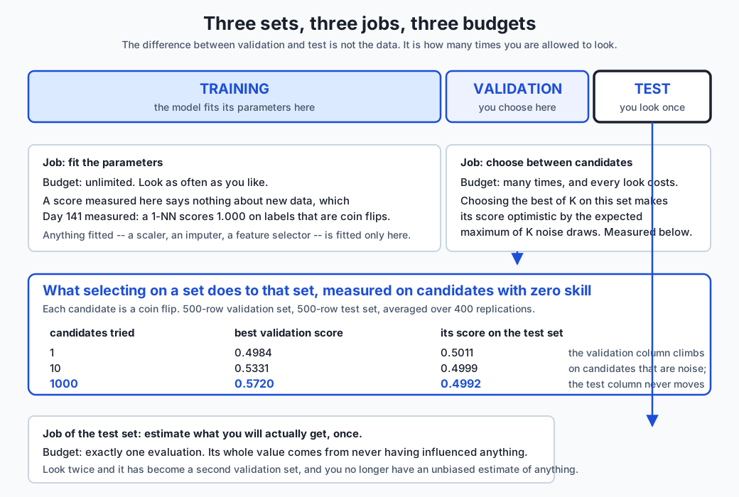
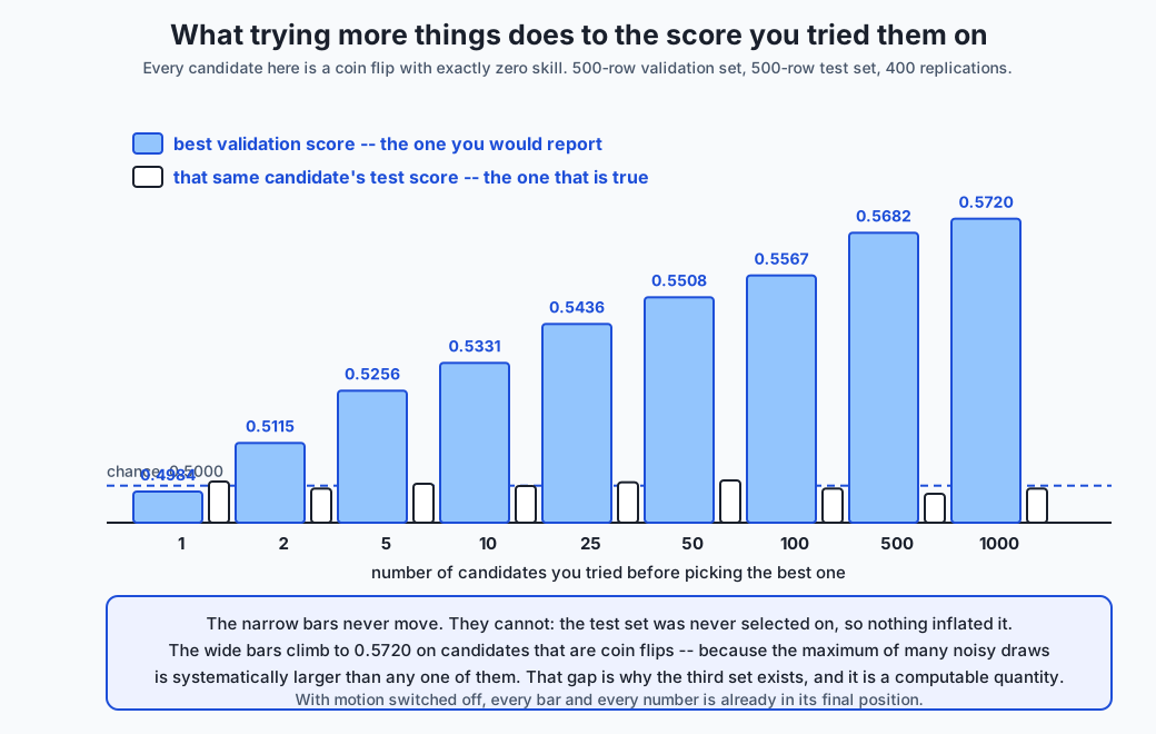
Each one is a coin flip — a fixed vector of random predictions, generated without ever looking at the data. Score all thousand on a 500-row validation set, keep whichever wins, and then check that winner against a test set it never touched:
     K   best-val   its-test   optimism
      1    0.4984     0.5011    -0.0028
     10    0.5331     0.4999    +0.0332
    100    0.5567     0.4992    +0.0575
   1000    0.5720     0.4992    +0.0728
Read the right-hand column first, because it is the control. It does not move. At one candidate or a thousand, the winner’s test score sits at chance, within three-thousandths of 0.5000 every time. Nothing inflated it, because nothing selected on it.
Now read the middle column. It climbs. Steadily, monotonically, all the way to 0.5720 — seven accuracy points above chance — on candidates that are literally coin flips.
Nobody cheated. No test label leaked. No feature was chosen using the answers. Every candidate genuinely has zero skill, and the reported number is genuinely 0.5720. The only thing that happened is that somebody tried a thousand things and kept the best one.
That is why there are three sets and not two, and it is the reason this lesson exists. A validation set is not a spare test set. It is the set you spend, and the arithmetic of spending it is not vague — it turns out to be exactly the expected maximum of K noise draws, a quantity you can compute in advance and budget for.
The rest of the day is the four ways a split goes wrong, each measured on this machine:
| The mistake | What it cost, here |
|---|---|
| not stratifying a rare class | 21 of 500 random splits had a test half with no positives at all |
| splitting rows when the unit is a person | +0.5648 — 0.9760 against 0.4112 |
| shuffling data that has a direction in time | +0.0728 on average; shuffling won 20 of 20 times |
| reading a trend off one holdout | one holdout swung 0.19 across seeds; 5-fold swung 0.0325 |
Day 143 showed that a wrong ordering of stages costs twenty-three points. Today shows that a wrong split can cost fifty-six.
The idea in plain language
Suppose you are hiring, and you have one very good interview question.
You use it on the first candidate. They do well. You use it on the second, the third, the fortieth. By the fortieth, something has gone quietly wrong: the question has been asked in the building forty times, people talk, and the answers are getting better in a way that has nothing to do with the candidates getting better. Your question has stopped measuring what it measured on day one, and it did not announce the change.
You have three options and they map exactly onto three sets.
Practice questions you can use as often as you like. Nothing is at stake, everybody knows the answers, and no measurement you take from them means anything about anybody’s ability. That is the training set.
A screening question you use many times, deliberately, to choose between candidates. It wears out — but wearing it out is the job, and you accept that its measurements drift optimistic as you reuse it. That is the validation set.
A sealed question you use exactly once, on the finalist, to find out what you have actually got. Its whole value comes from never having been used before. That is the test set, and it is the only one of the three that gives an honest number.
The thing that catches people out is that all three sets are the same kind of data. There is nothing special about the rows in the test set. The difference is entirely in how many times you are allowed to look at them — and a difference that lives in your discipline rather than in your data is a difference that is very easy to lose.
Historical background
Holding data back is old, and older than machine learning.
The idea appears in statistics as cross-validation, in work from the 1930s onward on assessing a fitted relationship against data it was not fitted to. The modern formulation is usually credited to Seymour Geisser and to Mervyn Stone, both writing in 1974, who set out the leave-one-out and k-fold schemes and — importantly — framed the question as predictive assessment rather than as goodness of fit. That distinction is the whole subject: a model can fit its data perfectly and predict nothing, which Day 141 measured at exactly 1.000.
The three-way split, as opposed to the two-way one, arrived with the practice of choosing between models. Once you are selecting a hyper-parameter, a feature set or an architecture, the set you select on has been used to fit something — just not the parameters — and the literature on selection bias and the optimism of the training error grew up around exactly that. Ambroise and McLachlan’s 2002 paper on gene-expression classification is the case that made it famous, and The Elements of Statistical Learning devotes a chapter to model assessment and selection in which the three-way split is stated plainly: train, validate, select; then test, once.
The winner’s curse — the phenomenon this lesson measures — was named in the 1970s by petroleum engineers analysing sealed-bid auctions for drilling rights. The winning bid is systematically too high, not because bidders are foolish, but because the winner is by construction the bidder whose estimate was most inflated. Capen, Clapp and Campbell published it in 1971. It is the same mathematics as picking the best of a thousand noisy validation scores, and Day 142 met it as a bandit arm with 274 pulls beating one with 1524.
The benchmark era supplied the cautionary tale at scale. A public test set that thousands of researchers evaluate against, over years, is a validation set with extra steps — every published improvement is a selection made on it. Work re-collecting fresh test sets for widely used image benchmarks in 2019 found accuracy dropping substantially on the new data, in a way consistent with a decade of collective selection rather than with outright cheating. Nobody looked at a test label. Everybody selected on the same set, and that was enough.
What it is — and what it is not
A split is a claim about independence, and everything in this lesson follows from taking that claim seriously.
When you hold out a test set, you are asserting that its rows tell you nothing about the training rows beyond what a fresh sample from the same population would. Every failure in this lesson is that claim being false in a way nobody checked.
Here is what each set is, precisely.
The training set is where parameters are fitted. Unlimited looks. Its score is not an estimate of anything, because Day 141 established that a 1-NN scores exactly 1.000 on labels that are coin flips. Crucially, anything fitted belongs here — a scaler, an imputer, an encoder, a feature selector, a decision threshold — which is Day 143’s ordering lesson restated as a property of the split.
The validation set is where you choose. Many looks, and every look costs you something measurable.
The test set is where you find out. One look. Its value comes entirely from never having influenced anything.
Now the things a split is not.
It is not a random partition of rows, in general. It is a random partition of independent units, and the row is the unit only when rows are independent. Today’s most alarming measurement is what happens when they are not:
  50 people, 20 rows each; each person's label is a coin flip
  row-wise random split : 0.9760
  group-aware split     : 0.4112
  accuracy invented     : +0.5648
  people appearing in BOTH halves of a row-wise split: 50 of 50
There is nothing generalisable in that dataset. Each person’s label is a coin flip, so a model can only score above chance on a person it has already met. A row-wise split reports 97.6 percent. The mechanism is that last line: with twenty rows each and a random quarter held out, every one of the fifty people appears on both sides. The model is not predicting; it is recognising.
A validation set is not a small test set. It is a resource you spend, and the spending is invisible in the number it returns.
And a test set is not reusable. Not “should not be” — is not. The second evaluation is a validation score wearing the word “test”, and today’s lab makes that mechanical:
class GatedTestSet:
    def evaluate(self, model) -> float:
        if self.evaluations >= 1:
            raise TestSetTouchedTwice(
                "the test set has already been used once; any further score is a "
                "validation score, not a test score"
            )
Why it was created and what problems it solves
Each of the three sets exists because a specific error occurs when it is missing, and each error has a measurement in today’s lab.
The training/test division solves memorisation, which Day 141 measured at 1.000 on coin flips.
The validation/test division solves selection bias, which is the headline measurement of this lesson and the one worth understanding properly rather than remembering as a rule.
Why does picking the best of K inflate the score? Because you are taking a maximum, and the maximum of several noisy estimates is systematically larger than any single one of them. Even when every candidate is identically worthless, some of them will have got lucky on the validation rows, and the one you keep is by definition the luckiest.
That is not hand-waving. It is a quantity. The standard error of an
accuracy measured on 500 rows at p = 0.5 is sqrt(0.25/500) = 0.0224. So
express the optimism in standard errors and compare it against the
expected maximum of K standard normal draws:
| K | measured, in SEs | E max of K normals | sqrt(2 ln K) |
|---|---|---|---|
| 2 | 0.55 | 0.55 | 1.18 |
| 10 | 1.48 | 1.54 | 2.15 |
| 100 | 2.57 | 2.50 | 3.03 |
| 1000 | 3.26 | 3.24 | 3.72 |
The measurement tracks the expected maximum closely at every K. The selection optimism is not a warning; it is a predictable quantity you can budget for before you run the sweep.
And note the third column, which is the honest finding here. The familiar
closed form sqrt(2 ln K) sits above the truth at every K tried — 3.03
where the answer is 2.50 at a hundred candidates. It is an asymptotic
approximation, correct in the limit and loose at any K you will actually
use. Today’s lab asserts the inequality rather than treating the formula
as the answer, because the simulation is the better estimate and the
measurement outranks the closed form.
Stratification solves the rare class. On a 5 percent positive class, across 500 random splits:
  random split     : {'mean': 0.0504, 'sd': 0.0265, 'min': 0.0, 'max': 0.16}
  stratified split : {'mean': 0.05, 'sd': 0.01, 'min': 0.04, 'max': 0.06}
  random splits whose test half held ZERO positives: 21 of 500
Both are unbiased — the means agree. The random split’s spread is 2.65 times wider, its worst case holds three times the population rate, and twenty-one splits in five hundred produced a test set with no positives whatsoever, on which recall is undefined and precision is a division by zero. Four percent of the time, a coin flip decides whether your evaluation is even computable.
Grouping solves the non-independent row, at fifty-six points.
Chronological splitting solves the direction of time. Which brings us to the finding that had to be reported carefully.
How it works
Why the maximum is biased, in one paragraph
Take K numbers drawn from the same distribution. Their average is an unbiased estimate of that distribution’s mean. Their maximum is not an estimate of anything except the maximum, and it grows with K.
Selecting a model on a validation set is taking a maximum. The score you
report is max over your candidates of a quantity that has noise in it,
and that maximum exceeds the true quality of the best candidate by an
amount depending only on how many candidates there were and how noisy each
measurement is. Both of those are things you know before you start.
Which gives a rule you can actually use: before running a sweep of K configurations, compute your validation set’s standard error and multiply it by the expected maximum of K normals. If that product exceeds the difference you are trying to detect, the sweep cannot answer your question, and no amount of care in running it will change that.
At 500 validation rows and a hundred candidates: 0.0224 × 2.50 = 0.056.
Fifty-six thousandths of accuracy, invented. If you are chasing a two-point
improvement, you are not measuring it.
What that formula assumes, and where it stops holding
Read the derivation again and two assumptions are doing all the work: the K candidates are independent, and they have no real skill, so their scores differ only by noise. Both are true by construction in the experiment above — the candidates are literally coin flips generated without looking at the data.
Neither is true of a real hyper-parameter sweep, and the difference is large. Day 147 runs this same formula against an actual 36-candidate sweep of skilled, correlated models and measures what it predicts against what happens:
  predicted optimism (SE of a CV fold x expected max of 36 normals): 0.0326
  measured drop, averaged over 20 seeds                            : -0.0001
Thirty-fold too large, and the measured drop is not even reliably positive. The reason is both assumptions failing at once. Adjacent hyper-parameter settings behave almost identically, so thirty-six candidates are nowhere near thirty-six independent draws — the effective K is far smaller. And candidates with genuine skill differ by more than noise, so the maximum is partly tracking something real rather than purely selecting for luck.
So treat the formula as an upper bound and a prompt, not a prediction. It is at its most accurate exactly where it is most alarming — many genuinely interchangeable candidates, a small validation set, a difference near the noise — and it overestimates as candidates become correlated or genuinely different from one another. The habit worth keeping is not the arithmetic but the question it forces: how many things did I try, and is the difference I am claiming larger than what trying that many things would have produced by itself?
Groups: when the row is not the unit
The group failure is worth walking through slowly, because it is the most expensive and the least visible.
The dataset is fifty people, twenty rows each. Each person has a signature — a characteristic point in feature space — and each person’s label is a coin flip. There is no relationship between the features and the label that could survive meeting a new person.
Split it row-wise and a 1-NN scores 0.9760. Split it by person and the same model scores 0.4112.
The mechanism is countable rather than subtle:
people appearing in BOTH halves of a row-wise split: 50 of 50Every single person. With twenty rows each and a random quarter held out, the chance that any one person’s rows all land on the same side is about two in a hundred thousand — so a fifty-person dataset will essentially never produce a clean split by accident. Each test row’s nearest neighbour is another row from the same person, carrying that person’s label. The model is doing a lookup.
The diagnosis is a question about the domain, not the data: what is the unit I want to generalise to? If it is a new patient, split by patient. A new customer, split by customer. A new document, split by document — not by sentence. Rows from the same unit are not independent, and a split that treats them as if they were is measuring recognition.
One honest note on that 0.4112, since it sits below chance. About twelve people land in the group-aware test half, each contributing twenty identical labels, so the estimate rests on roughly a dozen coin flips and wanders accordingly. The lab asserts the structural claim — group-aware below 0.5, row-wise far above it — rather than the value.
Time: the finding that had to be reported carefully
Data with a direction in time needs a chronological split, because deployment is chronological: you will always be predicting the future from the past, and a shuffled split lets the model interpolate between surrounding moments it will not have in production.
Today’s lab constructs a series in six regimes, each with its own rule mapping features to labels. A shuffled split scatters every regime across both halves. A chronological split asks the model to predict a regime it has never seen.
And here the honest reporting matters more than the number.
The first construction I ran gave an inflation of +0.1428. That is a striking figure, it fits the story, and quoting it would have been the forking-paths problem committed inside a lesson against exactly that. So the lab runs twenty independently generated series:
  shuffled split, mean       : 0.5961
  chronological split, mean  : 0.5233
  majority baseline, mean    : 0.5235
  inflation: mean 0.0728  sd 0.0596  min +0.0160  max +0.2557
  constructions where shuffling won: 20 of 20
Three things follow, and the third is the one worth carrying.
The direction is universal. Twenty out of twenty. Shuffling always flattered the model.
The size is not. From +0.016 to +0.2557, a factor of sixteen. The lab therefore splits the claim in two: one exercise asserts the direction, which held every time, and a second asserts the whole distribution.
And the honest verdict is stronger than the inflation number. The chronological score, 0.5233, is statistically indistinguishable from the majority baseline of 0.5235. Read chronologically, the model has learned nothing about the next regime. The shuffled split reports 0.5961 — comfortably above baseline, the shape of a weak but real signal. The mistake is not that the shuffled number is seven points too high. It is that it is on the wrong side of “does this work at all”.
Not every split mistake costs the same. Group leakage cost fifty-six points here and temporal leakage cost seven on average. Both are real; only one is an emergency, and a lesson that presented them as equally alarming would be less useful than one that ranks them.
One holdout, or many folds
The last structural question is how to spend the data you have.
Same dataset, same model, 200 different random splits:
  single holdout : {'mean': 0.7519, 'sd': 0.0381, 'min': 0.66, 'max': 0.85}
  5-fold         : {'mean': 0.7546, 'sd': 0.0061, 'min': 0.7375, 'max': 0.77}
The two agree on what they are estimating — the means differ by less than three-thousandths. What differs is the noise. The single holdout spans 0.66 to 0.85 across seeds, a swing of nineteen accuracy points, with nothing changing but which rows landed where. Cross-validation spans 0.7375 to 0.77 and is 6.23 times steadier.
Nineteen points is larger than most improvements anyone is chasing. If you are comparing two models on one holdout of a few hundred rows, the split is a bigger effect than the models.
Cross-validation buys that steadiness by making every row serve as test data exactly once, at a cost of k times the fits. On a laptop-scale problem that is the obvious trade. On something that takes a day to train it is not, and the honest alternative is a single holdout with an interval attached rather than a single holdout reported as a point.
How big must the test set be?
Decide this before you split, from the smallest difference you need to detect. The arithmetic is Day 117’s, arriving where the decisions are:
| test rows | standard error | measured | 95% half-width |
|---|---|---|---|
| 50 | 0.0505 | 0.0505 | ±0.0990 |
| 100 | 0.0357 | 0.0357 | ±0.0700 |
| 500 | 0.0160 | 0.0160 | ±0.0313 |
| 1000 | 0.0113 | 0.0112 | ±0.0221 |
| 5000 | 0.0050 | 0.0051 | ±0.0099 |
Theory and measurement agree to four decimal places at every size, which is worth pausing on: this is not a rule of thumb, it is a formula that predicts what actually happens.
Read the bottom column as a capability. A hundred-row test set carries a half-width of ±0.07, so two models five points apart are indistinguishable on it. To resolve two points at an accuracy of 0.85 you need 1225 rows; to resolve one point, 4899.
And note the shape: the error falls as one over root n, so quadrupling the test set halves the interval. Going from 500 to 1000 rows buys you a factor of 1.41. Going from 500 to 5000 buys you 3.2. There is no test-set size at which precision becomes free.
An everyday analogy
A driving test.
Lessons are the training set. You drive the same roundabout eleven times, your instructor corrects you, and nobody imagines your performance on the eleventh attempt says anything about your driving. Unlimited repetition is the point.
Mock tests are the validation set. Your instructor runs you through the real format to decide whether you are ready, and reruns it after you improve. Genuinely useful, and it wears out — by the fourth mock on the same route you know where the examiner looks for a mirror check, and your score improves in a way that is about the route rather than about your driving.
The test is the test set. One examiner, one route you have not practised, one attempt. Its value is that you did not prepare for that specific route.
The analogy earns its keep on the failures.
The group failure is being tested on the road outside your own house. Every row is a road you have driven a hundred times. You will pass brilliantly and the result predicts nothing about a strange town — 0.9760 against 0.4112.
The temporal failure is being tested in July having only ever driven in July. You will find out about ice in January, in production.
The stratification failure is a test route that happens to contain no roundabouts, when roundabouts are the thing you are bad at. Twenty-one routes in five hundred.
And the selection failure — today’s headline — is the one nobody notices. Take the test at forty different centres and report your best result. Every individual test was fair. Every examiner was honest. The number you quote is still not your driving ability, and it is inflated by an amount that depends only on how many centres you visited.
Examples in practice
Choosing the splitter
scikit-learn names the decision, which is genuinely helpful once you know what you are choosing between:
from sklearn.model_selection import (
    train_test_split,        # rows are independent, class balance is fine
    StratifiedShuffleSplit,  # rows are independent, a class is rare
    GroupShuffleSplit,       # rows share a unit: a person, a device, a document
    TimeSeriesSplit,         # the data has a direction
    StratifiedKFold,         # you want the steadier estimate
)
The instinct to build is that the default is a choice, not a starting
point. train_test_split is right when rows are independent and no class
is rare — and wrong, silently and expensively, otherwise.
A real grouped case, and how it is missed
Medical imaging is the standard example and the standard failure. A dataset of chest X-rays contains several images per patient — different dates, different views. Split by image and the same patient appears in both halves. The model learns to recognise patients, which it can do very well from anatomy that has nothing to do with the disease, and reports an excellent number.
What makes it hard to catch is that the score is plausible. It is not 1.000; it is 0.94, which is what a good model on a hard problem looks like. The only reliable defence is structural: ask what the unit is before you split, and check whether any unit appears on both sides. That check is one line, and today’s lab asserts it as a count.
Sizing a test set before collecting it
An engineer is asked whether a new model beats the current one. The current one is at 0.85. Product would accept a two-point improvement.
Before any modelling: two points at p = 0.85 needs 1225 test rows for a 95 percent interval of ±0.02. If only four hundred rows can be labelled, the interval is ±0.035 and the comparison cannot resolve the difference that was asked about. That is a finding, delivered on day one, and it is worth more than a model.
The benchmark that became a validation set
The most consequential real instance is collective. A public test set, thousands of researchers, years of published improvements — each paper selecting on the same rows. No individual looked at a test label. The aggregate is a selection over an enormous K, and today’s table says exactly what that does.
When fresh test data has been re-collected for widely used benchmarks, measured accuracy has dropped substantially. Model ranking has generally held up, which is the reassuring part; the absolute numbers have not, which is the part to remember before quoting one.
Implications: security, privacy, performance, scalability, and cost
The cost of a split mistake is entirely a cost of finding out late. A
model that reports 0.9760 in development and 0.4112 in production has cost
the build, the review, the deployment, the incident and the credibility of
the next project. GroupShuffleSplit costs one import.
Group splitting is a privacy control as well as an evaluation one. When rows are people and the same person appears in both halves, your model may be memorising individuals — which is both a broken evaluation and a disclosure risk, since membership-inference attacks target exactly that. The fix is the same for both problems.
Chronological splitting is a fraud-detection requirement, not a nicety. An evaluation that lets a model see the future is not a security control at all. Every backtest in an adversarial domain has to be chronological to mean anything.
Cross-validation costs k times the fits, which is the honest reason people use a single holdout. But the comparison to make is not compute against convenience — it is compute against a nineteen-point swing. If a fit is cheap, the holdout is a false economy. If it is expensive, the right answer is a single holdout with an interval, which costs nothing and stops you over-reading the number.
Test-set size is a budget decision made before labelling. The rows you need follow from the difference you must detect, and they scale as one over the square of the precision: doubling the precision quadruples the rows. Deciding this after labelling means discovering that your comparison was never possible.
And the largest cost is the one that never appears in a budget. Every traversal of the validation set spends some of it, and the spend is invisible in the result. A team that runs sweeps for six months and reports its best validation score has an artefact of the expected maximum of K noise draws — where K is the number of things they tried since January, which nobody counted. The countermeasure is to count.
Alternatives: free, open source, and commercial
scikit-learn’s splitters — used here
When to choose them: for essentially all in-memory work. Free, BSD-3-Clause licensed, no paid tier. Every measurement in this lesson uses them.
How to use them: every splitter exposes the same split(X, y, groups)
interface returning index arrays, so switching from a row-wise split to a
group-aware one is a one-line change:
from sklearn.model_selection import GroupShuffleSplit

splitter = GroupShuffleSplit(n_splits=1, test_size=0.25, random_state=0)
train, test = next(splitter.split(X, y, groups))
Watch for: train_test_split does not stratify unless you pass
stratify=y, and it has no idea your rows have groups. Both failures are
silent, and both are measured in today’s lab.
Nested cross-validation — described, and the honest note
When to choose it: when you must both tune and estimate on limited data. An inner loop selects, an outer loop scores, and the outer score is not contaminated by the selection — which is the correct fix for the optimism this lesson measures.
What it costs: the product of the two loops. Five outer folds and five inner folds is twenty-five times the fits.
Honest note: today’s lab does not implement nested cross-validation. It is the first extension exercise, and the lesson describes it from scikit-learn’s documentation without reproducing output for it.
Bootstrap and out-of-bag estimates — described from documentation
Resampling with replacement gives an alternative estimate and a natural interval; out-of-bag scoring in bagged ensembles gives one nearly free, since each tree has rows it never saw. Both are free and open source, both are in scikit-learn. Neither is measured here.
Managed experiment-tracking platforms — not used here
Commercial platforms record every run, every hyper-parameter and every score. The relevant capability for this lesson is that they can tell you K — how many configurations you actually tried — which is the number nobody remembers and which determines your selection optimism.
Free versus paid: most have a free tier for individuals and charge for teams. No price is quoted here, because these change by month and an unchecked figure is worse than none. Open-source self-hosted options exist and do the same job.
Comparison with related concepts
| Concept | What it does | How it relates |
|---|---|---|
| Holdout split | one train/test division | Simplest, and swings 0.19 across seeds on 400 rows |
| k-fold cross-validation | every row tests exactly once | 6.23 times steadier here, at k times the fits |
| Stratified k-fold | k-fold preserving class balance | The default for classification; costs nothing |
| Group k-fold | folds that never split a unit | The fix for the fifty-six-point failure |
| Time series split | expanding window, always forward | The fix for evaluating on the past |
| Nested cross-validation | an inner loop selects, an outer scores | The correct fix for selection optimism |
| Bootstrap | resample with replacement | Gives an interval directly; different bias properties |
| The winner’s curse | the maximum of noisy estimates is biased | The same mathematics, from auction theory |
Two rows deserve a closing note.
Stratified k-fold is free and should be your default for
classification. It has the same cost as k-fold, the same
interpretation, and strictly less variance. There is no reason to use
plain KFold on a classification problem.
And the winner’s curse row is not an analogy. It is the same computation. Day 142 met it as a bandit arm with 274 pulls beating one with 1524; today it is a validation score chosen from a thousand. In both cases the argmax over noisy estimates selects for inflation, and in both cases the size of the inflation is computable from the noise and the count.
When to use it — and when not to
Always ask what the unit of independence is, before anything else. Not “how much data do I have” but “what am I trying to generalise to”. If the answer is a new person, a new device, a new hospital, a new document — split by that, and check that no unit appears on both sides. That check is one line and it is worth more than most modelling.
Stratify by default on classification. Free, and it removes the twenty-one-in-five-hundred case where your evaluation is not even computable.
Split chronologically whenever the data has a direction, even when the measured inflation turns out small. The reason is not the average seven-point gap — it is that on this construction the chronological score was indistinguishable from the baseline while the shuffled one looked like a real signal. The mistake changes the verdict, not just the number.
Use cross-validation when a fit is cheap. On a laptop-scale problem, six times steadier for five times the compute is not a close call. When a fit is expensive, use a single holdout and report an interval — the half-width table above is all you need.
Keep the test set until you are finished selecting. Not until you are finished modelling — until you are finished choosing. And when you do look, look once and write down what you saw.
When you do not need three sets: when you are not selecting between anything. If you fit one model with settings fixed in advance and never compare it to an alternative, K is one, the optimism is zero, and two sets are enough. This is rarer than people think — trying two learning rates is K = 2 — but it is real, and the arithmetic tells you so rather than a rule.
The AI thread
Everything above becomes harder, not easier, at the scale of modern AI systems, and in three specific ways.
The test set may already be in the training data, and you cannot check. A model trained on a large fraction of the public internet has plausibly seen any benchmark published before its cutoff. A score on that benchmark is then partly a measure of memorisation, which is Day 141’s failure at a scale where the ordinary defence — inspect the training set — is not available. The practical response is to build private evaluation sets, and to hold back data collected after the cutoff. Both are expensive; neither is optional.
K is enormous and nobody is counting it. A public leaderboard is a validation set with thousands of participants selecting on it over years. Today’s table gives the shape of what that does, and the honest reading of any long-standing benchmark’s top scores includes an optimism term that nobody can compute because nobody knows K.
The unit of independence is genuinely hard to establish in text. Split a corpus by document and near-duplicates across documents still leak. Split by source and the same story is syndicated. Split by date and the same event is reported for a week. Every one of those is the group failure in a form where the groups are not labelled, and de-duplication becomes an evaluation control rather than a data-cleaning nicety.
The countermeasure in all three cases is the same as the one this lesson began with, and it is unglamorous: decide what you are generalising to, split by that, count how many times you have looked, and look at the final set once. The arithmetic does not care how large the model is.
Knowledge check
- A thousand candidates with zero skill are scored on a 500-row validation set. The best scores 0.5720. Explain where that number comes from, and predict what it would be with a 2000-row validation set.
- In today’s headline table, the test column never moves at any K. Why is that the load-bearing observation rather than an incidental one?
- Your validation set has 500 rows and you plan to try 100 configurations. Compute the accuracy you expect to invent, and say what it implies about detecting a two-point improvement.
sqrt(2 ln K)says 3.03 standard errors at K = 100; simulation says 2.50. Which should you use and why?- A row-wise split of the grouped dataset scores 0.9760 and a group-aware one scores 0.4112. State the mechanism in one sentence, and name the count that demonstrates it.
- Twenty-one of five hundred random splits produced a test set with no positives. What breaks, and what is the one-word fix?
- Shuffling beat chronological splitting in 20 of 20 constructions but the effect ranged from +0.016 to +0.2557. Why does the lesson report the distribution rather than the largest value?
- A single holdout on 400 rows spans 0.66 to 0.85 across seeds. What does that imply about a paper reporting a three-point improvement on one holdout of that size?
Hands-on exercise
Today’s lab, Three Sets, and Why, measures the selection optimism that
justifies a third set, then measures the four ways a split goes wrong.
Fourteen exercises. The first three build the headline result and connect it to the expected maximum of K noise draws. The next four measure stratification, groups and time. The last measure holdout variance, test-set sizing, and a test set that enforces its own one-look budget.
Build the environment, then work through starter/test_splits_claims.py,
replacing one pytest.skip at a time.
Expected output
The harness ends with:
---------------------------------------------------------------
14 checks, 0 failure(s)
and exits 0. pytest examples -q reports 18 passed, and
pytest starter -q reports 4 passed, 14 skipped until you begin.
The measured table includes:
     K   best-val   its-test   optimism   in SEs
      1    0.4984     0.5011    -0.0028    -0.13
   1000    0.5720     0.4992    +0.0728     3.26
  row-wise random split : 0.9760
  group-aware split     : 0.4112
  people appearing in BOTH halves of a row-wise split: 50 of 50
  constructions where shuffling won: 20 of 20
Validate your work
bash tests/run_tests.sh; echo "exit=$?"reports14 checks, 0 failure(s)andexit=0. Capture the harness’s own exit status..venv/bin/pytest examples -qreports18 passed..venv/bin/python3 examples/report_measurements.py | diff - expected-output/measured-values.txtproduces no output.- When you have finished every exercise,
pytest starter -qreports18 passed. - Break one assertion on purpose, confirm the harness fails, restore it.
Troubleshooting
The harness takes a while. It averages 400 replications at nine values of K and fits 400 models for the holdout comparison. No timing is asserted, so a slow machine changes nothing about whether it passes.
Your group-aware score is below 0.5. Expected, and asserted. About twelve people land in that test half, each contributing twenty identical labels, so the estimate is roughly a dozen coin flips.
Your temporal numbers differ. Almost certainly fine — the effect varies by a factor of sixteen across constructions, which is why the lab asserts the direction and the distribution rather than a figure.
sqrt(2 ln K) does not match. Correct, and asserted. It is an
asymptotic that is loose at every K you will use. The lab asserts that it
exceeds the simulated expectation.
import file mismatch. You ran pytest examples starter together.
Run them separately.
Common mistakes
Reading the validation column without the test column. The test column is the control; without it the climb proves nothing.
Treating the selection optimism as a warning rather than a quantity. It is computable in advance: standard error times the expected maximum of K normals.
Quoting the largest temporal effect. The lab deliberately does not, and exercise 4b asserts the whole distribution.
Concluding “never use a single holdout”. The lesson says use one with an interval when fits are expensive. The nineteen-point swing is an argument for reporting uncertainty, not for one method.
Practice assignment
Take an evaluation you already have and audit its split.
- Name the unit of independence. Not the row — the thing you want to generalise to. Then check whether any unit appears in both halves. One line, and the highest-value line in this assignment.
- Count K. How many configurations, features, thresholds and architectures have been tried against your validation set, in total, since the project started? Nobody knows this number; estimate it and write it down.
- Compute your selection optimism. Multiply your validation set’s standard error by the expected maximum of K normals for that K. Compare it to the improvement you are claiming. If the first exceeds the second, you have a finding.
- Size your test set for the decision. What is the smallest difference that would change what anyone does? How many rows does a 95 percent interval of that half-width need? Compare with what you have.
- Check for a direction in time, and if there is one, re-run your evaluation chronologically. Report both numbers and which side of your baseline each lands on.
The deliverable is the audit, not a better model.
Extension challenge
Pick one and measure it.
- Nested cross-validation. Implement it, and measure whether the optimism from exercise 1 disappears. Report the cost in fits.
- Find the break-even K. At what number of candidates does the selection optimism exceed a two-point true difference, for a 500-row validation set? Say what that implies about large sweeps.
- Scale the validation set. Repeat exercise 1 with 2000 rows and confirm the optimism scales with the standard error rather than staying fixed. Report the ratio.
- Leave-one-group-out. Replace
GroupShuffleSplitwithLeaveOneGroupOutand report both the mean and the spread across the fifty people. Say which is the more honest number to publish. - Make the temporal effect large deliberately. Find which property of a construction drives it — regime count, regime length, how different consecutive rules are — and give a rule of thumb for when a chronological split matters most.
- A gate that logs. Extend
GatedTestSetto record every attempted evaluation with a caller identifier. Then argue in two sentences whether a gate that logs is more useful than one that simply refuses.
Quiz
Q1. A thousand candidates, each a fixed vector of random predictions with exactly zero skill, are scored on a 500-row validation set. The best of them scores 0.5720. Where does that number come from?
- From overfitting: with a thousand candidates, at least one has genuinely learned the validation set
- From taking a maximum over noisy estimates -- some candidates got lucky on those 500 rows, and the one kept is by definition the luckiest
- From the validation set being too small; with 5000 rows the best would still score 0.5720
- From a bug: candidates with zero skill cannot average above 0.5
Show answer
Answer: B. From taking a maximum over noisy estimates -- some candidates got lucky on those 500 rows, and the one kept is by definition the luckiest
Each candidate's validation score is a draw with standard error 0.0224. The maximum of a thousand such draws sits about 3.26 standard errors above the mean, which is 0.0728 -- exactly the measured optimism. Nothing was learned: these are prediction vectors generated without ever seeing the data. And the score is not a bug, because the *average* candidate does score 0.5; it is the *maximum* that is biased. A larger validation set would shrink the standard error and therefore the optimism, which is the third option's mistake.
Q2. In that same experiment, the winner's test score sits within 0.003 of 0.5 for every value of K, from one candidate to a thousand. Why does that observation carry the argument?
- It shows the test set is larger than the validation set and therefore more reliable
- It shows the candidates were correctly generated, which is a sanity check on the setup
- It is the control: the test set was never selected on, so its stability proves the validation climb is selection and not some artefact of the experiment
- It shows the model generalises, since test performance did not degrade as K grew
Show answer
Answer: C. It is the control: the test set was never selected on, so its stability proves the validation climb is selection and not some artefact of the experiment
Without the test column, a rising validation score could be explained by almost anything -- a drifting generator, a bug in the scoring, an artefact of the averaging. The test column holds both sets to the same construction and differs in exactly one respect: nothing selected on it. That isolates selection as the cause. Both sets are 500 rows, so size is not the difference, and there is no model here to generalise -- the candidates are coin flips.
Q3. Your validation set has 500 rows and you plan to try 100 configurations. What accuracy should you expect to invent, and what does it mean for detecting a two-point improvement?
- About 0.056 -- the standard error 0.0224 times the expected maximum of 100 normals, 2.50 -- so a two-point improvement cannot be resolved by that sweep
- About 0.002, since the optimism is roughly one over the number of validation rows
- None, provided you also keep a test set; the test set corrects the validation optimism
- About 0.068 -- the standard error times sqrt(2 ln 100), which is 3.03
Show answer
Answer: A. About 0.056 -- the standard error 0.0224 times the expected maximum of 100 normals, 2.50 -- so a two-point improvement cannot be resolved by that sweep
The optimism is the validation set's standard error multiplied by the expected maximum of K noise draws, and both are known before you start. At 0.0224 and 2.50 that is 0.056 -- more than twice the improvement being chased, so the sweep cannot answer the question. The sqrt(2 ln K) figure is the tempting wrong answer and is addressed in the next question. And a test set does not correct the validation optimism; it simply gives you a separate honest number, which is precisely why both exist.
Q4. The closed form sqrt(2 ln K) predicts 3.03 standard errors of optimism at K=100. Simulation of the expected maximum of 100 normals gives 2.50, and the measurement gives 2.57. Which should you use?
- sqrt(2 ln K), because a closed form is exact where a simulation is an approximation
- Neither -- disagreement between them means the whole framework does not apply here
- The average of the two, since each carries error in a different direction
- The simulated expectation, because sqrt(2 ln K) is an asymptotic that is loose at every K you would actually use, and the measurement confirms the simulation rather than the formula
Show answer
Answer: D. The simulated expectation, because sqrt(2 ln K) is an asymptotic that is loose at every K you would actually use, and the measurement confirms the simulation rather than the formula
sqrt(2 ln K) is correct in the limit as K grows without bound and overestimates at finite K -- by 0.53 standard errors here, which is a fifth of the answer. The simulation is a direct estimate of the quantity you want and the measurement lands within 0.07 of it. This lesson's lab asserts the inequality -- that the closed form exceeds the simulation -- rather than treating the formula as truth, on the standing principle that when a measurement and a textbook disagree, the measurement wins.
Q5. Fifty people, twenty rows each, and every person's label is a coin flip so nothing is generalisable. A row-wise random split scores 0.9760; a group-aware split scores 0.4112. What is the mechanism, and which count demonstrates it?
- The row-wise split has more training data, and the count is 750 training rows against 700
- The 1-NN memorises its training rows, and the count is the 1000 rows in the dataset
- Every one of the fifty people appears in both halves, so each test row's nearest neighbour is another row from the same person carrying that person's label
- The group-aware split has fewer test rows and therefore a noisier estimate, and the count is the twelve people in its test half
Show answer
Answer: C. Every one of the fifty people appears in both halves, so each test row's nearest neighbour is another row from the same person carrying that person's label
With twenty rows per person and a random quarter held out, the chance that one person's rows all land on the same side is about two in a hundred thousand -- so the count of people in both halves is 50 of 50, and the lab asserts it. The model is doing a lookup rather than predicting. Training-set size is not the difference, and while the group-aware estimate is genuinely noisy -- twelve people, hence a score below chance -- noise explains the wobble, not the fifty-six-point gap.
Q6. Across 500 random splits of a 5-percent positive class, 21 produced a test half containing no positives at all. What breaks, and what is the fix?
- Recall is undefined and precision divides by zero; the fix is to stratify the split
- Accuracy becomes meaningless; the fix is to use a larger model
- Nothing breaks -- a test set with no positives simply measures specificity, which is still informative
- The training set becomes imbalanced; the fix is to oversample the minority class
Show answer
Answer: A. Recall is undefined and precision divides by zero; the fix is to stratify the split
With no positives in the test half there is no true positive and no false negative, so recall has a zero denominator and precision divides by zero whenever the model predicts a positive. Stratifying costs nothing, keeps the same mean positive rate, and cuts the spread from a standard deviation of 0.0265 to 0.0100 -- and never produced an empty test half in 500 splits. Oversampling addresses a different problem, in the training half, and does not fix an evaluation set that cannot be evaluated.
Q7. A shuffled split beat a chronological one in all 20 constructions tested, but the effect ranged from +0.016 to +0.2557. Why does the lesson report the whole distribution rather than the largest value?
- Because the largest value came from a construction with a bug, so it was excluded
- Because averages are conventionally preferred to extremes when reporting results
- Because quoting the seed that produced the biggest effect would be the forking-paths problem committed inside a lesson against it -- and the direction, which held 20 of 20, is the defensible claim
- Because the mean of 0.0728 is the true effect size and the extremes are measurement error
Show answer
Answer: C. Because quoting the seed that produced the biggest effect would be the forking-paths problem committed inside a lesson against it -- and the direction, which held 20 of 20, is the defensible claim
The first construction tried gave +0.1428, which would have made a striking headline. Choosing it after seeing the results is exactly selecting on the outcome, which is what this lesson measures elsewhere. So the lab asserts the direction in one exercise and the full distribution -- mean, standard deviation, minimum and maximum -- in another. Note also that the extremes are not measurement error: they are real variation between datasets, which is why the practical lesson is that split mistakes do not all cost the same.
Q8. A single holdout on 400 rows spans 0.66 to 0.85 across 200 random seeds, on identical data and an identical model. What does that imply about a reported three-point improvement measured on one such holdout?
- That the improvement is real but understated, since a single holdout is conservative
- That the improvement is smaller than the split-to-split variation, so the holdout cannot distinguish it from having drawn a luckier split
- That the model is overfitting, since a stable model would give a stable holdout score
- That the test set is too large, and a smaller one would give a tighter estimate
Show answer
Answer: B. That the improvement is smaller than the split-to-split variation, so the holdout cannot distinguish it from having drawn a luckier split
Nineteen accuracy points of swing come from nothing but which rows landed where. A three-point difference measured once, on one split of that size, is comfortably inside the noise. Five-fold cross-validation on the same data spans 3.25 points and is 6.23 times steadier, which is the practical answer when fits are cheap; when they are not, the answer is a single holdout reported with an interval. The swing is a property of the split, not of the model, and a smaller test set would widen the interval rather than narrow it.
Glossary
- Training set
- The rows a model fits its parameters on, and the only rows anything fitted may see -- a scaler, an imputer, an encoder, a feature selector or a decision threshold included. Unlimited looks, and a score measured here estimates nothing.
- Validation set
- The rows you choose between candidates on. Many looks are permitted and every look costs something measurable: the score on this set is inflated by the expected maximum of K noise draws, where K is how many things you tried.
- Test set
- The rows that tell you what you will actually get. Exactly one look. Its entire value comes from never having influenced anything, so the second evaluation is a validation score wearing the word test.
- Selection bias
- The optimism created by keeping the best of several candidates measured on the same set. Not a vague hazard but a computable quantity -- measured here at 0.0728 for a thousand candidates that were literally coin flips.
- Winner's curse
- The systematic upward bias of an argmax taken over noisy estimates: the winner is whichever estimate was most inflated. Named in 1971 for sealed-bid oil leases, met on Day 142 as a bandit arm, and met today as a validation score.
- Expected maximum of K draws
- The quantity selection optimism actually equals, once expressed in standard errors. Simulated here at 0.55, 1.54, 2.50 and 3.24 standard errors for K = 2, 10, 100 and 1000, tracking the measurement to within 0.2 at every K.
- Standard error of an accuracy
- sqrt(p times one minus p, divided by n) -- how much an accuracy estimate wobbles from the split alone. 0.0224 on 500 rows at p = 0.5. Theory matched 20000 measured draws to four decimal places at every size tried.
- Stratified split
- A split preserving each class's proportion in both halves. Costs nothing, has the same mean as a random split, and cuts the spread by a factor of 2.65 here -- while never once producing the empty test half a random split produced 21 times in 500.
- Group split
- A split that never puts rows from the same unit -- person, device, document, hospital -- on both sides. The fix for the most expensive failure in this lesson: 0.9760 row-wise against 0.4112 group-aware, because all fifty people were in both halves.
- Unit of independence
- The thing you want to generalise to, which is the thing you must split by. The row is the unit only when rows are independent, and deciding this is a question about the domain rather than about the data.
- Chronological split
- Training on the past and testing on the future, because deployment is chronological. Shuffling beat it in 20 of 20 constructions here, and the chronological score turned out indistinguishable from the majority baseline where the shuffled one looked like real signal.
- k-fold cross-validation
- Dividing the data into k parts so every row serves as test data exactly once. Six times steadier than a single holdout here, at k times the fits, and estimating the same quantity -- the two means agreed to within 0.003.
- Holdout variance
- How much a single train/test estimate moves when only the split changes. Measured at 0.0381 standard deviation and a 0.19 range on 400 rows -- larger than most improvements anyone is chasing.
- Nested cross-validation
- An inner loop that selects and an outer loop that scores, so the outer estimate is not contaminated by the selection. The correct fix for the optimism this lesson measures, at the product of the two loops in compute.
- Test-set sizing
- Deciding how many test rows you need from the smallest difference that would change a decision, before splitting. 1225 rows for plus or minus 0.02 at an accuracy of 0.85; 4899 for plus or minus 0.01.
- One-over-root-n
- The rate at which a sampling error shrinks. Quadrupling a test set halves its interval rather than quartering it, so precision never becomes cheap -- going from 500 rows to 5000 buys a factor of 3.2.
- Benchmark overfitting
- What happens when a public test set is selected on by thousands of researchers over years. No individual sees a test label; the aggregate is a selection over an enormous and uncounted K, and re-collected test data has shown substantial accuracy drops.
- Evaluation budget
- The number of times a held-out set may be consulted before its estimate stops being honest. One for a test set. Enforceable mechanically -- today's GatedTestSet refuses the second look and deliberately does not advance its counter on a refusal.
- Data leakage through the split
- Information about the test rows reaching training through the split itself rather than through a feature: a shared person, a shared moment in time, a fitted transform applied before the cut. All three are silent and all three inflate.
- Optimism
- The gap between a score measured on data that influenced a choice and the score on data that did not. In this lesson it has a sign, a size, a formula and a control -- which is what distinguishes it from a warning.
Sources and further reading
- Cross-validation: evaluating estimator performance -- scikit-learn user guide — scikit-learn developers (accessed 2026-08-27)
- GroupShuffleSplit -- scikit-learn API reference — scikit-learn developers (accessed 2026-08-27)
- StratifiedKFold -- scikit-learn API reference — scikit-learn developers (accessed 2026-08-27)
- TimeSeriesSplit -- scikit-learn API reference — scikit-learn developers (accessed 2026-08-27)
- Common pitfalls and recommended practices, including data leakage — scikit-learn developers (accessed 2026-08-27)
- The Elements of Statistical Learning, chapter 7 on model assessment and selection -- free PDF from the authors — Trevor Hastie, Robert Tibshirani and Jerome Friedman, Springer (accessed 2026-08-27)
- Cross-validation (statistics) — Wikipedia (accessed 2026-08-27)
- Winner's curse -- the same mathematics, from auction theory — Wikipedia (accessed 2026-08-27)
- Random Generator -- NumPy reference, on stream compatibility — NumPy developers (accessed 2026-08-27)
Kept in this browser, no account needed. Your progress page turns the whole record into one link you can bookmark or open on another device.